Similarity Inner Solutions for the Pulsar Equation

Abstract

Lie symmetries are applied to classify the source of the magnetic field for the Pulsar equation near to the surface of the neutron star. We find that there are six possible different admitted Lie algebras. We apply the corresponding Lie invariants to reduce the Pulsar equation close to the surface to an ordinary differential equation. This equation is solved either with the use of Lie symmetries or the application of the ARS algorithm for singularity analysis to write the analytic solution as a Laurent expansion. These solutions are called inner solutions.

I Introduction

Pulsars are one of the most impressive observable celestial objects in the sky. They are assumed to be rotating neutron stars which emit radio signals. However, their importance follows from the fact that they are physical laboratories which provide extreme conditions of strong magnetic fields which cannot be reproduced on Earth.

The structure of the strong magnetic fields in a Pulsar is described by a scalar function which satisfies the elliptic second-order partial differential equation pulsar1 ; pulsar2 ,

$$\left(1-x^{2}\right)\left(\Psi_{,xx}+\Psi_{,zz}\right)-\frac{1+x^{2}}{x}\Psi_{,x}+F\left(\Psi\right)=0,$$ (1)

where the singularities at $x=0$ and $x=1$ represent the centre of the star, ($x$ is the radius coordinate) and the surface of the pulsar is located at $x=1$. Function $F\left(\Psi\right)$ is related to the profile of the magnetic field for the polar coordinate pulsar1 . Equation (1) is also known as the relativistic force-free Grad-Shafranov equation ppl1 .

In order to arrive at such a simple scalar equation, (1), for the magnetic field, various Ansätze have been assumed for the physical state of the star. In particular it has been assumed that pulsar1 : (a) the system is axisymmetric and time-independent; (b) the electrons and the ions have a well-defined velocity and density; (c) there are no gravitational or particle collision effects; (d) inertial forces have been considered and (e) it is assumed that the surface of the uniformly rotating star is a perfect conductor.

Because of the nonlinearity and the existence of the two singular points, the Pulsar equation, (1), cannot be integrated in general and only few solutions are known in the literature. Originally, an asymptotic analytical solution which describes the magnetic field near to the surface of the star was presented by Michel in pulsar2 . This was also the main inspiration for the recent works of Uzdensky pl3 and Gruzinov pl4 . In pl3 an interesting discussion of the physical state of the boundary conditions is given. However, numerical solutions which describe the global evolution of the Pulsar equation have been presented in the literature. One of the first numerical force-free solutions was derived by Contopoulos et al. pl5 , while other numerical solutions can be found in pl6 ; pl7 ; pl8 ; pl9 and references therein.

In this work we are interested to apply the powerful method of Lie symmetries Stephani ; Bluman in order to study the existence of invariant solutions for the Pulsar equation near to the singularity, $x=1,~{}$and to find analytical asymptotic solutions, the so-called similarity solutions. In particular, we classify the source of the magnetic field, i.e. function $F\left(\Psi\right)$, such that the Pulsar equation, near to the singularity, $x=1$, be invariant under the action of one-parameter point transformations. This kind of classification was firstly introduced by Ovsiannikov ovsiannikov and has been applied to various physical systems for the determination of new analytical solutions, for instance see ref1 ; ref2 ; ref3 ; ref4 ; ref5 ; ref6 ; ref7 ; ref8 ; ref9 ; ref10 ; qm1 ; qm2 ; qm3 ; qm4 and references therein, for various applications of the Lie symmetry classification in Physics.

The novelty of Lie symmetries is that symmetries can be used to define invariant surfaces and to reduce the number of dependent variables – for partial differential equations – or to reduce the order of the differential equation for ordinary differential equations. Hence new integrable systems can be constructed and new analytical solution to be determined. The plan of the paper follows.

In Section II the basic properties and definitions for the Lie (point) symmetries of differential equations are presented. In the same Section we perform the classification of the Lie symmetries of the pulsar equation near to the surface of the star and we find that there are six different admitted groups of point-transformations which leave the pulsar equation invariant for six different functional form of the source, $F\left(\Psi\right)$. The context of singularity analysis is discussed which is used in subsequent Sections to prove the integrability of some of the reduced differential equations. The application of the Lie symmetries and the determination of the similarity inner solutions is performed in Section III. New asymptotic analytic solutions near to the surface of the star are presented. Finally in Section IV we discuss our results and we draw our conclusions.

II Lie symmetry analysis

For the convenience of the reader we present the basic properties and definitions of Lie point symmetries of differential equations and more specifically we discuss the case of second-order differential equations of the form $\mathbf{A\equiv}A\left(x^{k},\Psi,\Psi_{,i},\Psi_{,ij}\right)=0$, where $x^{k}$ are the independent variables and $\Psi$ is the dependent variable with first derivative $\frac{\partial\Psi}{\partial x^{i}}=\Psi_{,i}$.

Let

$$X=\xi^{i}\left(x^{k},u\right)\partial_{i}+\eta\left(x^{k},\Psi\right)\partial_{u},$$ (2)

be the generator of the local infinitesimal one-parameter point transformation,

$$\bar{x}^{k} =x^{k}+\varepsilon\xi^{i}\left(x^{k},\Psi\right),$$ (3)

$$\bar{\eta} =\eta+\varepsilon\eta\left(x^{k},\Psi\right).$$ (4)

Then $X$ is called a Lie symmetry for the differential equation, $\mathbf{A}$, iff

$$X^{\left[2\right]}A=\lambda A$$ (5)

in which $X^{\left[2\right]}$ is called the second prolongation/extension in the jet-space and is defined as

$$X^{\left[1\right]}=X+\left(D_{i}\eta-\Psi_{,k}D_{i}\xi^{k}\right)\partial_{\Psi_{,i}}+\left(D_{i}\eta_{j}^{\left[i\right]}-\Psi_{jk}D_{i}\xi^{k}\right)\partial_{\Psi_{,ij}}.$$ (6)

The novelty of Lie symmetries is that they can be used to determine similarity transformations, i.e. differential transformations where the number of independent variables is reduced Bluman . The similarity transformation is calculated with the use of the associated Lagrange’s system,

$$\frac{dx^{i}}{\xi^{i}}=\frac{du}{\Psi}=\frac{d\Psi_{i}}{\Psi_{\left[i\right]}}=...=\frac{d\Psi_{ij..i_{n}}}{\Psi_{\left[ij...i_{n}\right]}}.$$ (7)

Solutions of partial differential equations which are derived with the application of Lie invariants are called similarity solutions. In this specific work we use the Lie symmetries to reduce the Pulsar equation to a second-order differential equation. For this equation we shall analytic solutions by using the symmetry approach and, if we fail, we apply the singularity analysis.

II.1 Singularity analysis

Singularity analysis is another powerful mathematical method which is applied to study the integrability of differential equations and to present the solutions of differential equations in algebraic form, in particular by using Laurent expansions around a movable singularity.

Singularity analysis is also known as the Painlevé Test Painleve1 ; Painleve2 ; Painleve3 ; Painleve4 and has been applied in various problems for the study of integrability of  given differential equations.

Ablowiz, Ramani and Segur Abl1 ; Abl2 ; Abl3 systematized the Painlevé Test in a simple algorithm, also known as the ARS algorithm. The main feature of the ARS algorithm is its simplicity. It consists of three main algebraic stems: (a) determination of leading-order behaviour; (b) determination of resonances and (c) consistency of Laurent expansion. For every step of the algorithm there are various criteria which should be applied, these criteria are summarized in the review of Ramani et al. buntis .

If a given differential equation passes the three steps of the ARS algorithm, then we conclude that the given differential equation is algebraically integrable. However, should the differential equation fail the ARS algorithm, we cannot make a conclusion about the integrability of the differential equation. While the ARS algorithm is straightforward on its application, one of the main disadvantages is that it depends upon the coordinates in which the given equation is defined, for a recent discussion we refer the reader to anleach .

II.2 Pulsar equation near to the singularity

We define the new coordinate, $y=x-1$, in order to move the surface of the star to $y=0$. It follow, $y>0$, when $x>1$ and $y<0$ , when $x<1$. In the new coordinates the Pulsar equation (1) becomes

$$y\left(2+y\right)\left(\Psi_{,yy}+\Psi_{,zz}\right)+\frac{\left(2+2y+y^{2}\right)}{1+y}\Psi_{,y}-F\left(\Psi\right)=0.$$ (8)

Near to the surface with $y\simeq 0$, (8) is approximated by the simpler form pulsar2

$$2y\left(\Psi_{,yy}+\Psi_{,zz}\right)+2\Psi_{,y}-F\left(\Psi\right)=0.$$ (9)

This is the equation which Michel pulsar2 used to find the first analytical expression for the force-free magnetosphere and inspired the later works of pl3 ; pl4 . Equation (9) is the one that we use to perform the symmetry classification.

Moreover, we follow pl3 ; pl4 and we work on the polar-like coordinates

$$y=r\sin\theta~{},~{}z=r\cos\theta,$$ (10)

where equation (9) takes the form

$$2r\sin\theta\left(\Psi_{,rr}+\frac{1}{r^{2}}\Psi_{,\theta\theta}\right)+2\left(2\sin\theta+\frac{\cos\theta}{r}\right)\Psi_{,r}-F\left(\Psi\right)=0.$$ (11)

Hence the surface is indicated when $r=0$ or $\theta=0$. We continue with the classification of the sources, $F\left(\Psi\right)$, such that equation (11) be invariant under one-parameter point transformations, i.e. Lie symmetries exist, while in the following section we discuss the application of the Lie symmetries by performing reduction of the equation with the use of the Lie invariants.

II.3 Symmetry classification

For the second-order differential equation (11) the symmetry condition (5) provides that for arbitrary function, $F_{A}\left(\Psi\right)=F\left(\Psi\right)$, the differential equation admit the unique symmetry vector

$$Y=\cos\theta\partial_{r}-\frac{\sin\theta}{r}\partial_{\theta}.$$

That vector field corresponds to the translation symmetry, $\partial_{z}$, in the original coordinates, for equation (8) which is also a symmetry of equation (1). Reduction with the use of the symmetry vector $Y$ leads to solutions which are independent of the $z-$direction and are not of special interest.

However, for specific functions, $F\left(\Psi\right)$, the differential equation (11) can be invariant under a higher dimensional Lie algebra. In particular we find five different cases:

• When the source is constant, i.e. $F_{B}\left(\Psi\right)=F_{0}$, the differential equation (11) admits four plus infinity symmetries, these are.

  $$X_{1}=\partial_{r}~{},~{}X_{2}=Y~{},~{}X_{3}=r^{2}\cos\theta\partial_{r}+r\sin\theta\partial_{x}-r\cos\theta~{}\Psi\partial_{\Psi}$$

  $$X_{4}=\Psi\partial_{\Psi}~{},~{}X_{\infty}=b\left(r,\theta\right)\partial_{\Psi},$$ (12)

  where $b\left(r,\theta\right)$ is a solution of equation (11). The last two symmetries, i.e. $X_{4}$ and $X_{\infty},$ denote the linearity of equation (11). The Lie Brackets of the admitted algebra are given in Table 1

Table 1: Lie Brackets of the admitted Lie symmetries for the free pulsar equation 11

$\left[\cdot,\cdot\right]$ $X_{1}$ $X_{2}$ $X_{3}$ $X_{4}$ $X_{1}$ $0$ $0$ $0$ $0$ $X_{2}$ $0$ $0$ $-X_{3}$ $X_{4}$ $X_{3}$ $0$ $X_{3}$ $0$ $2X_{2}-X_{1}$ $X_{4}$ $0$ $-X_{4}$ $-2X_{2}+X_{1}$ $0$

• For linear source, $F_{C}\left(\Psi\right)=F_{1}\Psi,~{}$the differential equation admits two plus infinity symmetries, those are $X_{2}~{},~{}X_{4}~{}$and$~{}X_{\infty}.$

• Moreover, for the power-law source, $F_{F}\left(\Psi\right)=F_{1}\Psi^{\frac{1}{N}+1},~{}N\neq 0,\frac{1}{2},-1,~{}$Pulsar equation near to the surface admits two Lie point symmetries, these are

  $$X_{2}~{},~{}X_{\left(N\right)}=r\partial_{r}-N\Psi\partial_{\Psi}$$ (13)

  with Lie Bracket $\left[X_{2},X_{\left(N\right)}\right]=X_{2}$.

• In the special case for which$~{}N=\frac{1}{2}$ in the latter case, or $F_{E}\left(\Psi\right)=F_{1}\Psi^{3},~{}$the Pulsar equation (11) is invariant under a three-dimensional Lie algebra with elements the vector fields $X_{2},~{}X_{\left(1/2\right)},~{}X_{3},~{}$and Lie Brackets as are presented in Table 2.

Table 2: Lie Brackets of the admitted Lie symmetries for the pulsar equation with cubic-law force

$\left[\cdot,\cdot\right]$ $X_{2}$ $X_{\left(1/2\right)}$ $X_{3}$ $X_{2}$ $0$ $-X_{(1/2)}$ $X_{3}$ $X_{\left(N\right)}$ $X_{(1/2)}$ $0$ $2X_{2}$ $X_{3}$ $-X_{3}$ $-2X_{2}$ $0$

• Finally, for the exponential source, $F_{F}\left(\Psi\right)=F_{1}e^{-\frac{1}{C}\Psi}$, $C\neq 0,$ the Pulsar equation admits two Lie point symmetries,

  $$X_{2}~{},~{}\bar{X}_{\left(C\right)}=r\partial_{r}+C\partial_{\Psi}\text{.}$$

  with Lie Bracket $\left[X_{2},\bar{X}_{\left(C\right)}\right]=X_{2}$. We mention that the exponential-lie source was introduced in ppl1 as a jet model.

We continue with the application of the Lie symmetry vectors to determine analytical solutions of the Pulsar equation (11). The solutions that we determine are valid as first approximations of the general solution near to the surface of the star. In particular, near to the surface of the star, $y\simeq 0$, the differential equation can be seen as a singular pertubative equation and the theory of singular perturbative differential equations sper1 ; sper2 can be applied in order to justify the approximation of the analytical solution. The solutions near to the point $y\simeq 0$ are called inner solutions sper1 .

III Similarity solutions

As we discussed in the previous Section, for every Lie symmetry we can define a surface where the solution is independent of one of the variables, that is, define similarity variables.

For arbitrary source, $F\left(\Psi\right)$, from the vector field $\partial_{z}$ the invariant solution is the one where $\Psi\left(y,z\right)=\Psi\left(y\right)$ and the resulting differential equation is the ordinary differential equation

$$2y\Psi_{,yy}+2\Psi_{,y}-F\left(\Psi\right)=0.$$ (14)

That is not a solution of special interest. Hence we proceed with our analysis by using the remainder of the symmetry vectors.

III.1 Invariant solutions for constant source

The case of constant source also covers the free-source problem when $F_{0}=0$. Indeed in equation (9) for $F\left(\Psi\right)=F_{0}$ we can replace $\Psi\rightarrow\Psi+\frac{F_{0}}{2}y$. Then the source-free case follows. From table 1 it follows that there are four possible reductions which we can perform. They are: (a) reduction with the symmetry vector $X_{1}+\mu X_{4}$; (b) reduction with $X_{2}+\mu X_{4}$; (c) reduction with $X_{3}+\mu X_{4}$; and (d) reduction with $X_{3}+\mu X_{2}$.  For each of these reductions the reduced equation is a linear second-order differential equation which can be integrated easily.

III.1.1 Reduction with $X_{1}+\mu X_{4}$

The first possible reduction of the source-free Pulsar equation (11) provides the solution to be

$$\Psi_{1}\left(r,\theta\right)=r^{\mu}\Sigma\left(\theta\right),$$ (15)

where $\Sigma\left(\theta\right)$ satisfies the ordinary differential equation

$$\Sigma_{,\theta\theta}+\cot\theta~{}\Sigma_{,\theta}+\mu\left(\mu+1\right)\Sigma=0$$ (16)

the closed-form solution of which is given in terms of the Legendre functions as

$$\Sigma\left(\theta\right)=\sigma_{1}P_{\mu}\left(\cos\theta\right)+\sigma_{2}Q_{\mu}\left(\cos\theta\right)$$ (17)

in which $P_{\mu}\left(\theta\right),$ $Q_{\mu}\left(\theta\right)$ denote the Legendre functions.

For special values of the parameter $\mu$ the solution (17) can be simplified as follows

$$\Sigma\left(\theta\right)=\sigma_{1}+\sigma_{2}\ln\left(\frac{1-\cos\theta}{\sin\theta}\right),~{}\mu=0,$$ (18)

$$\Sigma\left(\theta\right)=\sigma_{1}\cos\theta+\sigma_{2}\left(1-\frac{\cos\theta}{2}\ln\left(\frac{\cos\theta-1}{\cos\theta+1}\right)\right),~{}\mu=1.$$ (19)

It is important to mention that in general the parameter, $\mu$, can be any complex number and, when it is imaginary, solution (15) becomes periodic as follows $\Psi\left(r,\theta\right)=\exp\left(i|\mu|\ln r\right)\Sigma\left(\theta\right).~{}$

Solution (15) is well-known in the literature and was derived by Michel in pulsar2 . In particular for $\mu=\frac{1}{2}$ solution (15) provides a magnetic field which diverges as the inverse square root of $r$ such that the total energy of the magnetic field remains finite at the surface of the star, i.e. when $y=0$. That is a physical condition which imposes a boundary condition and restricts the free parameters of the solution.

The analytical solutions which are presented in the following Sections are new in the literature, but, as we see, they do not provide explicitly any law of the form $\Psi\simeq r^{\frac{1}{2}}$.

III.1.2 Reduction with $X_{2}+\mu X_{4}$

Consider now reduction with the Lie symmetry vector, $X_{2}+\mu X_{4}$.  The invariant solution is calculated in Cartesian coordinates to be

$$\Psi_{2}\left(y,z\right)=\Sigma\left(y\right)e^{\mu z},$$ (20)

where the function $\Sigma\left(y\right)$ is

$$\Sigma\left(y\right)=\sigma_{1}J_{0}\left(\mu y\right)+\sigma_{2}Y_{0}\left(\mu y\right),$$ (21)

in which $J_{m}\left(y\right),~{}Y_{m}\left(y\right)$ denote the Bessel functions of the first and second kind, respectively.

III.1.3 Reduction with $X_{3}+\mu X_{4}$

Reduction with the Lie symmetry vector, $X_{3}+\mu X_{4}$, provides the invariant solution

$$\Psi_{3}\left(r,\theta\right)=\frac{1}{r}e^{\mu r\cos\theta}\Sigma\left(\frac{\sin\theta}{r}\right),$$ (22)

where again the function $\Sigma\left(\frac{\sin\theta}{r}\right)$ is expressed n terms of the Bessel functions $J_{m}~{}$and$~{}Y_{m}$ as

$$\Sigma\left(\frac{\cos\theta}{r}\right)=\sigma_{1}J_{0}\left(\mu\frac{\sin\theta}{r}\right)+\sigma_{2}Y_{0}\left(\mu\frac{\sin\theta}{r}\right).$$ (23)

III.1.4 Reduction with $X_{3}+\mu X_{2}$

The last possible reduction that we can perform in the source-free scenario is with the use of the Lie symmetry vector, $X_{3}+\mu X_{2}.$ The invariant solution is calculated to be

$$\Psi_{4}\left(r,\theta\right)=\frac{\Sigma\left(\sigma\right)}{\sqrt{\mu r^{2}-1}},$$ (24)

where the new independent variable $\sigma=\sigma\left(r,\theta\right)$ is defined as $\sigma=\frac{r\sin\theta}{\mu r^{2}-1}$. The function $\Sigma\left(\sigma\right)$ satisfies the second-order differential equation

$$2\sigma\left(4\mu\sigma^{2}+1\right)\Sigma_{,\sigma\sigma}+2\left(1+12\mu\sigma^{2}\right)\Sigma_{,\sigma}+6\mu\sigma\Sigma=0,$$ (25)

the solution of which is expressed in terms of the Legendre functions $P\left(\sigma\right),~{}Q\left(\sigma\right),$ that is,

$$\Sigma\left(\sigma\right)=\sigma_{1}P_{-\frac{1}{4}}\left(8\mu\sigma^{2}+1\right)+\sigma_{2}Q_{-\frac{3}{4}}\left(8\mu\sigma^{2}+1\right).$$ (26)

The source-free equation, (11), is linear, a property that follows also from the existence of the symmetry vectors $X_{4}$ and $X_{\infty}$. Hence the general solution can be written as a sum of the specific invariant solutions $\Psi_{1},~{}\Psi_{2},~{}\Psi_{3}$ and $\Psi_{4}$ calculated above, over all the possible values of the free parameters $\mu$ for each solution. However, the general solution is restricted only when initial/boundary conditions are applied in the problem.

In the following lines, the reduction process is applied for the remainder of the cases provided by the Lie symmetry classification.

III.2 Invariant solutions for linear source

For the linear source, $F_{C}\left(\Psi\right)=F_{1}\Psi$, it is possible to perform only one reduction with the symmetry vector $X_{2}+\mu X_{4}$. The invariant solution is calculated in Cartesian coordinates to be

$$\Psi\left(y,z\right)=e^{\mu z}\left(\Psi_{1}M_{a,0}\left(2i\mu y\right)+\Psi_{2}W_{a,0}\left(2i\mu y\right)\right),$$ (27)

where $\alpha=\frac{iF_{1}}{4\mu};$ and $M_{a,b},$ $W_{a,b}$ are Whittaker functions.

III.3 Invariant solutions for power-law source

For the power-law source, $F_{D}\left(\Psi\right)=F_{1}\Psi^{\frac{1}{N}+1}$   , we perform reduction by using the Lie symmetry vector $X_{\left(N\right)}$.  The reduced equation is calculated to be

$$2\sin\theta~{}\Sigma_{,\theta\theta}+2\cos\theta~{}\Sigma_{,\theta}+\left(2N\left(N-1\right)\sin\theta-F_{1}\Sigma^{\frac{1}{N}}\right)\Sigma=0$$ (28)

while the solution of the Pulsar equation, (11), is expressed as

$$\Psi\left(r,\theta\right)=r^{-N}\Sigma\left(\theta\right).$$ (29)

The reduced equation, (28), has been derived before in pl3 ; pl4 and actually the power-law source can describe the magnetic field of the Pulsar after the surface boundary. More specifically, in pl4 it was assumed that, when the source-free axisymmetric pulsar magnetosphere closes, there exists a boundary condition in order for the solution of the power-law source to continue to describe the magnetic field. Hence with that assumption it was found that the value of $N$ is approximately $N\simeq-2.4,$ such that $\Psi\simeq r^{2.4}$ pl4 .

It is interesting to comment here that solutions (15) and (29) were derived before without any knowledge of the symmetries of the differential equation (11). Moreover, those specific invariant solutions satisfy the boundary conditions imposed by the physics of the neutron star.

On the other hand, in the coordinates $\left\{y,z\right\}$, the reduced solution can be written equivalently as $\Psi\left(y,z\right)=y^{-N}\Lambda\left(\sigma\right)$, where $\theta=\arcsin\sigma$, and $\Lambda\left(\sigma\right)$ now satisfies the equation

$$2\sigma\left(1-\sigma^{2}\right)\Lambda_{,\sigma\sigma}+2\left(1+2\sigma^{2}\right)\Lambda_{,\sigma}+\left(2\sigma N\left(N-1\right)-F_{1}\Lambda^{\frac{1}{N}}\right)\Lambda=0.$$ (30)

This nonlinear equation does not admit any Lie symmetry and for that we apply the singularity analysis to study the integrability and write the analytical solution.

Equation (30) is a nonautonomous equation. With the new change of variables, $\sigma=Y\left(s\right)$, $\Lambda\left(\sigma\right)=Y_{,s}\left(s\right),~{}$we increase the order of the differential equation, but the new equation is autonomous. We apply the steps of the ARS algorithm.

We determine the leading-order behaviour to be $Y_{A}\left(s\right)=Y_{0}s^{\frac{1}{1+N}}$, for $N\neq-1,$ where $Y_{0}$ is an arbitrary constant. Hence once expects one of the resonances to be zero.

As far as concerns the resonances they are calculated to be

$$q_{1}=-1~{},~{}q_{2}=0~{},~{}q_{3}=\frac{2N-1}{1+N},$$ (31)

which means that the differential equation passes the singularity test and the  analytical solutions is expressed by a Right Painlevé series for $N\in\left(-\infty,-1\right)\cup\left(\frac{1}{2},+\infty\right)$ with step which depends on the value $N$.

In order to perform the consistency test, we select $N=2$ which means that the third resonance is $q_{3}=1$. Hence the step of the Laurent expansion is $\frac{1}{3},$ and the Painlevé series which describes the solution is

$$Y\left(s\right)=Y_{0}s^{\frac{1}{3}}+Y_{1}s^{\frac{2}{3}}+Y_{2}s+Y_{3}s^{\frac{4}{3}}+{\displaystyle\sum\limits_{I=4}^{\infty}}Y_{I}s^{\frac{1+I}{3}}.$$ (32)

The three integration constants are: the position of the singularity and the coefficients $Y_{0}$ and $Y_{2}$.  The rest of the coefficients $Y_{J}$ are functions of $Y_{0}$, $Y_{2}$. Hence, equation (28) is integrable though the singularity analysis.

However, there exists also a second leading-order behaviour, which is $Y_{B}\left(s\right)=Y_{0}s^{\frac{1}{2-N}},~{}$with arbitrary $Y_{0}$ and for all the values of $N$, such that $N\neq 2$. The resonances are calculated to be

$$\bar{q}_{1}=-1~{},~{}\bar{q}_{2}=0~{},~{}\bar{q}_{3}=\frac{2N-1}{N-2}$$ (33)

from which we infer that equation (28) is integrable.

III.4 Invariant solutions for the cubic source

When the power-law source has a cubic law, that is, $F_{E}\left(\Psi\right)=F_{1}\Psi^{3}$, then from the symmetry classification we saw that the Pulsar equation admits an extra Lie symmetry vector field. The reduction with the vector field $X_{3}$, provides the invariant solution

$$\Psi\left(r,\theta\right)=\frac{1}{r}\Sigma\left(\frac{\sin\theta}{r}\right),$$ (34)

where function $\Sigma$ satisfies the nonlinear differential equation

$$2\xi\Sigma_{,\xi\xi}+2\Sigma_{,\xi}-F_{1}\Sigma^{3}=0~{},~{}\xi=\frac{\sin\theta}{r}.$$ (35)

Equation (35) admits the vector field $X_{\left(1/2\right)}$ as Lie (point) symmetry. The application of $X_{\left(1/2\right)}$ gives

$$w\left(\alpha\right)=\xi^{\frac{3}{2}}\Sigma_{,\xi}~{},~{}\alpha=\xi^{\frac{1}{2}}\Sigma,$$ (36)

where now $w\left(\alpha\right)$ satisfies the first-order differential equation

$$\left(2+\alpha\right)w_{,\alpha}-w-F_{0}\alpha^{3}=0,$$ (37)

which is an Abel’s equation of the second kind.

The solution of this Abel’s equation cannot be written in a closed-form. However, differential equation (35) can be solved with the singularity analysis and the generic solution is given in algebraic form. Hence we apply the ARS algorithm. by firstly making the equation an autonomous third-order equation with the transformation $\xi=Y\left(s\right)$ and $\Sigma\left(\xi\right)=Y\left(s\right)_{,s}.$ Equation (35) is written as

$$YY_{,s}Y_{,sss}-2Y\left(Y_{,ss}\right)^{2}+\left(Y_{,s}\right)^{2}Y_{,ss}-F_{1}\left(Y_{,s}\right)^{6}=0.$$ (38)

For this equation we perform the new change of coordinates $Y\left(s\right)=\frac{1}{Z\left(s\right)},$ where we find that the leading-order behaviours are $Z\left(s\right)=Z_{0}s^{p}$, with $p_{1}=-1$ and $p_{2}=-2.$ In both cases, $Z_{0}$ is an arbitrary constant.

For $p_{1}$ the ARS algorithm provides the resonances

$$q_{1}=-1~{},~{}q_{2}=0~{},~{}q_{3}=\frac{3}{2}$$ (39)

which means that the the general solution is given by a Right Painlevé expansion with step $\frac{1}{2}$, that is

$$Z\left(s\right)=Z_{0}s^{-1}+Z_{1}s^{-\frac{1}{2}}+Z_{2}+Z_{3}s^{\frac{1}{2}}+{\displaystyle\sum\limits_{I=4}^{\infty}}Z_{I}s^{-1+\frac{I}{2}}$$ (40)

with free parameters $Z_{0}$ and $Z_{3}$. Note that the third constant of integration denotes the position of the movable singularity. Finally the consistency test provides that $Z_{1}=0$, $Z_{2}=-\frac{F_{1}}{2Z_{0}^{2}}$, $Z_{4}=\frac{5\left(F_{1}\right)^{5}}{4Z_{0}^{5}}~{}etc.$

As far as concerns the second leading-order behaviour, $p_{2}$, we find that the resonances are

$$\bar{q}_{1}=-1~{},~{}\bar{q}_{2}=-2~{},~{}\bar{q}_{3}=-4$$ (41)

and, while once expects one of the resonances to be zero, because $Z_{0}$ is arbitrary, that is not true. Hence the ARS algorithm for the leading-order term $p_{2}$ fails and solution (40) is the only solution which can be constructed by the ARS algorithm.

In Fig. 1 the density plot of the invariant solution (34) is given in space of variables $\left\{y,z\right\}$.

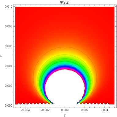
Figure 1: Density plot of $\Psi\left(y,z\right)$ for the analytical solutions (34). The figure is for initial conditions where $\Sigma\left(0\right)=0$ and $\Sigma_{,\xi}\left(0\right)>0$.

For completeness we mention that reduction with the symmetry vector $X_{\left(1/2\right)}$ provides the same solution as that of the power-law source $F_{D}\left(\Psi\right)$ for $N=\frac{1}{2}$.

III.5 Invariant solutions for exponential source

Finally for the power-law source, $F_{F}\left(\Psi\right)=F_{1}e^{-\frac{1}{C}\Psi}$, we apply the invariants of the Lie symmetry vector field $\bar{X}_{\left(C\right)}$, which provide us with the invariant solution

$$\Psi\left(r,\theta\right)=\ln r^{-C}+\Sigma\left(\theta\right),$$ (42)

where $\Sigma\left(\theta\right)$, satisfies the nonlinear second-order differential equation

$$2\sin\theta~{}\Sigma_{,\theta\theta}+2\cos\theta~{}\Sigma_{,\theta}-F_{1}e^{-\frac{1}{C}\Sigma}-2C\sin\theta=0.$$ (43)

As before we prefer to work with the coordinates $\left\{y,z\right\}$  and write the invariant solution as

$$\Psi\left(y,z\right)=\ln y^{C}+\Lambda\left(\sigma\right)~{},~{}\text{with ~{}}\theta=\arcsin\sigma,$$ (44)

in which function $\Lambda\left(\sigma\right)$ satisfies the differential equation

$$2\sigma\left(1-\sigma^{2}\right)\Lambda_{,\sigma\sigma}+2\left(1-2\sigma^{2}\right)\Lambda_{,\sigma}-2C\sigma-F_{1}e^{-\frac{1}{C}\Lambda}=0.$$ (45)

Equation (45) has no symmetries and in order to prove the integrability we apply the ARS algorithm. Indeed, under the change of variables $\sigma=Y\left(s\right)$, $\Lambda\left(\sigma\right)=C\ln Y_{,s}\left(s\right),$ the leading-order behaviour is calculated to be $Y\left(s\right)=Y_{0}s^{\frac{1}{1+C}}$, with resonances

$$\bar{q}_{1}=-1,~{}\bar{q}_{2}=0~{},~{}\bar{q}_{3}=-\frac{1}{1+C}.$$ (46)

Finally we apply the consistency test of the ARS algorithm for various values of the parameter $C,$ and we infer that for $C\neq-1$ the differential equation (45) passes the singularity test and its solution can be expressed in terms of a Laurent expansion.

In Fig. 2 the density plot of the invariant solution (34) is given in space of variables $\left\{y,z\right\}$.

Figure 2: Density plot of $\Psi\left(y,z\right)$ for the invariant solution (42). The plots are for initial conditions $\Sigma\left(0\right)=0$ and $\Sigma_{,\theta}\left(0\right)>0$ (left fig.) and $\Sigma_{,\theta}\left(0\right)<0$ (right fig.)

IV Conclusions

In this work we applied two powerful mathematical methods in order to determine analytical solutions for the Pulsar equation near to the surface of the neutron star. More specifically we applied the Lie symmetry analysis to classify the form of the source for the magnetic field in the Pulsar equation such that the resulting equation admit Lie (point) symmetries, that is, be invariant under the action of one-parameter point transformations. From the classification process, we found that the (inner) Pulsar equation can be invariant under the action of six different Lie algebras.

For each of the vector fields followed by the classification scheme we used the (zeroth-order) Lie invariants to reduce the number of the independent variables for the differential equation and write it as an ordinary differential equation. That equation could be solved in all the cases with the use of symmetries or with the application of the ARS algorithm. In particular the ARS algorithm was applied to prove the integrability for some of the reduced equations and write the analytical solution in a form of Laurent expansion.

The solutions that we derived are asymptotic solutions of the Pulsar equation (1) near to the surface of the neutron star. Only two of the solutions were derived before in the literature and these Lie invariant solutions provide a finite magnetic field in the surface of the neutron star. The new asymptotic solutions can be used as toy-models for the viability of numerical approximations for the elliptic equation (1)

In a forthcoming work we wish to study the boundary conditions which should be satisfied in order that the new Lie invariant solutions be solutions of the complete problem. Finally the physical implications of those solutions is a subject for a future study.

- (1) E.T. Scharlemant and R.V. Wagoner, Astroph. J. 182, 951 (1973)
- (2) F.C. Michel, Astroph. J. 180, L133 (1973)
- (3) S. Appl and M. Camenzind, Astron. Astrophys. 274, 699 (1993)
- (4) D.A. Uzdensky, Astroph. J. 598, 446 (2003)
- (5) A. Gruzinov, Phys. Rev. Lett. 94, 021101 (2005)
- (6) I. Contopoulos, D. Kazanas and C. Fendt, Astroph. J. 511, 351 (1999)
- (7) A.N. Timokhin, MNRAS 368, 1055 (2006)
- (8) L. Bratek and M. Kolonko, Astroph. Sp. Sci. 309, 231 (2007)
- (9) S.A. Petrova, MNRAS 427, 514 (2012)
- (10) Y. Takamori, H. Okawa, M. Takamoto and Y. Suwa, PASJ 66, 25 (2014)
- (11) H. Stephani, Differential Equations: Their Solutions Using Symmetry, Cambridge University Press, New York, (1989)
- (12) G.W. Bluman and S. Kumei, Symmetries of Differential Equations, Springer-Verlag, New York, (1989)
- (13) L. V. Ovsiannikov, Group Analysis of Differential Equations, Academic Press, New York, (1982)
- (14) K.S. Govinder and P.G.L. Leach, J. Non. Math. Phys. 14, 443 (2007)
- (15) C.M. Mellin, F.M. Mahomed and P.G.L. Leach, Int. J. Non-Linear Mech. 29, 529 (1994)
- (16) G.E. Prince and C.J. Eliezer, J. Phys. A: Math. Gen. 14, 587 (1981)
- (17) M. Tsamparlis and A. Paliathanasis, Gen. Relativ. Gravit. 42, 2957 (2010)
- (18) G.Z. Abebe, S.D. Maharaj and K.S. Govinder, Gen. Relativ. Gravit. 46, 1650 (2014)
- (19) T. Christodoulakis and N. Dimakis, J. Phys. Conf. Ser. 68, 012040 (2007)
- (20) A.H. Kara and F.M. Mahomed, Int. J. Theor. Phys. 34, 2267 (1995)
- (21) P.G.L. Leach, J. Phys. A: Math. Gen. 13, 1991 (1980)
- (22) N. Kallinikos and E. Meletidou, J. Phys. A: Math. Theor. 46, 305202 (2013)
- (23) A.H. Kara and F.M. Mahomed, Int. J. Theor. Phys. 34, 2267 (1995)
- (24) J. Belmonte-Beitia, V.M. Perez-Garcia, V. Vekslerchik and P.J. Torres, Phys. Rev. Lett, 98 064102 (2007)
- (25) L. Gagnon and P. Winternitz, J. Phys. A: Math. Gen. 21 1493 (1988)
- (26) L. Gagnon and P. Winternitz, J. Phys. A: Math. Gen. 22 469 (1988)
- (27) R.O. Popovych, N.M. Ivanova and H. Eshraghi, J. Math. Phys. 45 3049 (2014)
- (28) P. Painlevé, Leçons sur la théorie analytique des équations différentielles (Leçons de Stockholm, 1895) (Hermann, Paris, 1897). Reprinted, Oeuvres de Paul Painlevé, vol. I, Éditions du CNRS, Paris, 1973.
- (29) P. Painlevé, Bulletin of the Mathematical Society of France 28, 201 (1900)
- (30) P. Painlevé, Acta Math. 25, 1 (1902)
- (31) P. Painlevé, Comptes Rendus de la Académie des Sciences de Paris 143, 1111 (1906)
- (32) M.J. Ablowitz, A. Ramani and H. Segur, Lettere al Nuovo Cimento 23, 333 (1978)
- (33) M.J. Ablowitz, A. Ramani and H. Segur, J. Math. Phys. 21, 715 (1980)
- (34) M.J. Ablowitz, A. Ramani and H. Segur, J. Math. Phys. 21, 1006 (1980)
- (35) A. Ramani, B. Grammaticos and T. Bountis, Physics Reports, 180, 159 (1989)
- (36) A. Paliathanasis and P.G.L. Leach, IJGMMP 13, 1630009 (2016)
- (37) A.N. Tikhonov, Sbornic. Math. 31, 575 (1952)
- (38) N. Fenichel, J. Differential Equations 31, 53 (1979)