Population transfer via a dissipative structural continuum

Abstract

We propose a model to study quantum population transfer via a structural continuum. The model is composed of two spins which are coupled to two bosonic modes separately by two control pulses, and the two bosonic modes are coupled to a common structural continuum. We show that efficient population transfer can be achieved between the two spins by using a multi-level stimulated Raman adiabatic passage (STIRAP) across the continuum, which we refer to as straddle STIRAP via continuum. We also consider the stability of this model against different control parameters and show that efficient population transfer can be achieved even in presence a moderate dissipation.

I Introduction

Complete population transfer serves transition population of quantum states from initial state to target state, which plays an important role in quantum physics. A lot of research efforts have been devoted to study complete population transfer in various situations. For instance, complete population transfer among quantum states of atoms and molecules is very active researching area in quantum optics and atom optics Kuklinski et al. (1989); Bergmann et al. (1998); Huang et al. (2017). Furthermore, it is also a fundamental technique in quantum computation and quantum information processing, including superconducting qubits Falci et al. (2017); Chen et al. (2018); Kumar et al. (2016), Bose-Einstein condensates Helm et al. (2018), NV centers in diamond Chakraborty et al. (2017), quantum dots and quantum wells in semiconductor Dory et al. (2016). Another very important application of complete population transfer is to achieve power or intensity inversion in classical systems, which is widely used in waveguide couplers Huang et al. (2014), wireless energy transfer Rangelov et al. (2011), polarization optics Dimova et al. (2015) and electrons, surface plasmon polaritons in graphene system Huang et al. (2018a, b). For a recent review one can refer to Bergmann et al. (2019).

A standard approach for population transfer is stimulated Raman adiabatic passage (STIRAP), which was originally proposed in three-level systems, two of which are coupled to an intermediate energy level by two spatially overlapping pulses in counter-intuitive order. The remarkable dominance of STIRAP are that i) it is extremely robust against fluctuations of the control parameters of the laser pulses and ii) the intermediate energy level is not populated which makes the scheme robust against the decay Vitanov et al. (2001, 2017).

Various generalizations have made to apply STIRAP technique to special situations. STIRAP via multi-intermediate levels or continuum (multi-level STIRAP, also called straddle-STIRAP Vitanov et al. (1998)) has been considered in atomic system Peters and Halfmann (2007); Vitanov and Stenholm (1999); Rangelov et al. (2007a) and waveguide couplers system Dreisow et al. (2009); Longhi (2008). STIRAP into continuum, where the third energy level is replace by continuous energy levels, has also been considered Rangelov et al. (2007b).

In this paper, we propose a model to study population transfer via a continuum. The model contains two spins which are coupled to two bosonic modes separately by two controled laser pulses, while the two bosonic modes are indirectly coupled via a structured continuum. Compared to previous literatures, our model differs in that: i) the two energy levels are replaced by two spins, as a result, the population transfer becomes state transfer between the two spins; ii) instead of directly coupling the two energy levels with the continuum, in our approach the laser pulses directly couples the two spins with two bosonic modes, which could be single-mode cavities or phonons, and then the two bosonic modes are coupled to a continuum with constant coupling strengths; iii) dissipative continuum has been considered. This model has potential applications in chemical physics Deng et al. (2016) and quantum information Contreras-Pulido and Aguado (2008). In addition, this model allows us to study state transfer between two qubits via a dissipative environment, which could play an important role in quantum computation and quantum information processing. We demonstrate that straddle-STIRAP can be utilized to perform efficient population transfer in our model (see Fig. 2 and Fig. 3). And we show the robustness of our approach with respect to parameters of controlling laser pulses (see Fig. 4) and dissipation rate (see Fig. 5).

Our paper is organized as follows. In Sec.II, we introduce our model and the equation of motion for the straddle-STIRAP via a continuum. In Sec.III, we numerically solve the quantum master equation for our model, and show the effectiveness of the popular transfer against changing the parameters of the model. We conclude in Sec.IV.

II Model

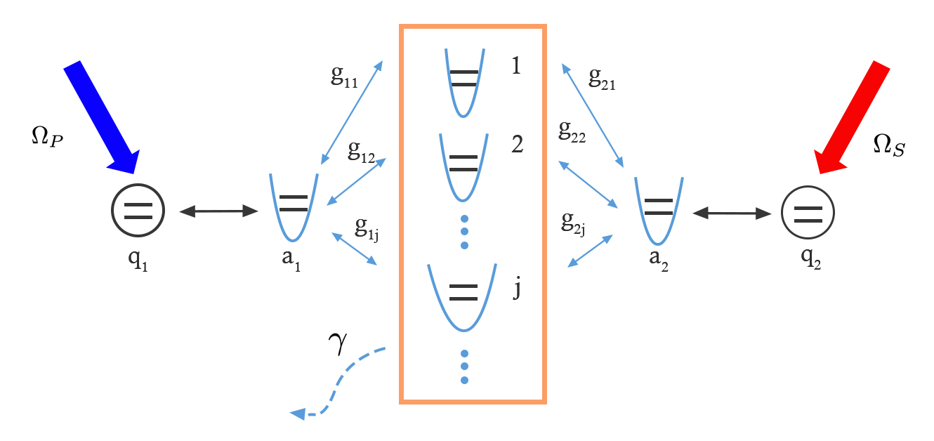
Figure 1: Population transfer between two qubits $q_{1}$ and $q_{2}$. The two qubits are coupled to two bosonic modes $\hat{a}_{1}$ and $\hat{a}_{2}$ respectively by two controled laser pulses $\Omega_{P}(t)$, $\Omega_{S}(t)$. The bosonic modes $\hat{a}_{1}$ and $\hat{a}_{2}$ are indirectly coupled through a bosonic structural continuum, with a particle loss rate $\gamma$.

Our model consists of two spins which are coupled to two bosonic modes by two controled laser pulses. The two bosonic modes are both coupled to a bosonic continuum with phenomenological spectrum functions. The bosonic continuum is initially in the vacuum state and is subjected to a particle loss rate of $\gamma$. The Hamiltonian of the whole system can be written as

$$\hat{H}(t)= \frac{\omega_{q,1}}{2}\hat{\sigma}^{z}_{1}+\frac{\omega_{q,2}}{2}\hat{\sigma}^{z}_{2}+\omega_{a,1}\hat{a}^{\dagger}_{1}\hat{a}_{1}+\omega_{a,2}\hat{a}^{\dagger}_{2}\hat{a}_{2}+$$

$$\Omega_{P}(t)(\hat{a}^{\dagger}_{1}\hat{\sigma}^{-}_{1}+\hat{a}_{1}\hat{\sigma}^{+}_{1})+\Omega_{S}(t)(\hat{a}^{\dagger}_{2}\hat{\sigma}^{-}_{2}+\hat{a}_{2}\hat{\sigma}^{+}_{2})+$$

$$\int_{\omega}d\omega\omega\hat{b}^{\dagger}(\omega)\hat{b}(\omega)+$$

$$\int_{\omega}d\omega\sqrt{J_{1}(\omega)}\left(\hat{a}_{1}\hat{b}^{\dagger}(\omega)+\hat{a}^{\dagger}_{1}\hat{b}(\omega)\right)+$$

$$\int_{\omega}d\omega\sqrt{J_{2}(\omega)}\left(\hat{a}_{2}\hat{b}^{\dagger}(\omega)+\hat{a}^{\dagger}_{2}\hat{b}(\omega)\right),$$ (1)

where we have set $\hbar=1$. Here $\omega_{q,1}$ and $\omega_{q,2}$ are the energy differences of qubit 1 and qubit 2. $\omega_{a,1}$ and $\omega_{a,2}$ denote the oscillation frequencies of the two bosonic modes $\hat{a}_{1}$ and $\hat{a}_{2}$. $J_{1}(\omega)$ and $J_{2}(\omega)$ are the spectral densities for the coupling between the two modes $\hat{a}_{1}$, $\hat{a}_{2}$ and the bosonic continuum. We have used a linear density of states assumption for the continuum without loss of generality since the density of states can be absorbed into the spectral densities De Vega and Alonso (2017). In this work we consider the phenomenological spectral densities which are defined as follows

$$J_{1}(\omega)=g\omega^{\eta_{1}};J_{2}(\omega)=g\omega^{\eta_{2}},$$ (2)

with a threshold $\omega_{c}$ such that $J_{1}(\omega)=J_{2}(\omega)=0,\forall\omega>\omega_{c}$. The exponent $\eta<1$, $\eta=1$ and $\eta>1$ correspond to the sub-ohmic, ohmic and super-ohmic couplings respectively. We also consider the situation where the bosonic continuum loses particles with a rate $\gamma$, which can be modeled by the Lindblad form of dissipation $\mathcal{D}$

$$\mathcal{D}(\hat{\rho})=\gamma\int_{\omega}d\omega\left[2\hat{b}(\omega)\hat{\rho}\hat{b}^{\dagger}(\omega)-\{\hat{b}^{\dagger}(\omega)\hat{b}(\omega),\hat{\rho}\}\right].$$ (3)

The dynamics of the system is thus described by the following quantum master equation

$$\frac{d\hat{\rho}(t)}{dt}=-{\rm i}\left[\hat{H}(t),\hat{\rho}(t)\right]+\mathcal{D}(\hat{\rho}(t)).$$ (4)

Throughout this paper, we assume that $\omega_{q,1}=\omega_{q,2}=\omega_{a,1}=\omega_{a,2}=\Delta$. The initial state of the dynamical evolution is denoted as

$$\hat{\rho}_{i}=\hat{\rho}(-\infty)=|\psi_{i}\rangle\langle\psi_{i}|,$$ (5)

with

$$|\psi_{i}\rangle=|1^{q_{1}},0^{a_{1}},\vec{\mathbb{0}}^{b},0^{a_{2}},0^{q_{2}}\rangle,$$ (6)

where we have use $1^{q_{i}},i=1,2$ to denote the spin up state for the two spins $q_{1}$ and $q_{2}$, $0^{a_{i}},i=1,2$ to denote the vacuum state for the two bosonic modes $\hat{a}_{1}$ and $\hat{a}_{2}$, and $\vec{\mathbb{0}}^{b}$ to denote the vacuum state for the bosonic continuum $\hat{b}(\omega)$. The final state after the evolution is denoted as $\hat{\rho}_{f}=\hat{\rho}(\infty)$, while the targeting final state is written as

$$\bar{\hat{\rho}}_{f}=|\psi_{f}\rangle\langle\psi_{f}|,$$ (7)

with

$$|\psi_{f}\rangle=|0^{q_{1}},0^{a_{1}},\vec{\mathbb{0}}^{b},0^{a_{2}},1^{q_{2}}\rangle.$$ (8)

We define $\mathcal{F}_{1}(t)$ to be the fidelity between $\hat{\rho}(t)$ and $\hat{\rho}_{i}$

$$\mathcal{F}_{1}(t)=\langle\psi_{i}|\hat{\rho}(t)|\psi_{i}\rangle,$$ (9)

which is the population of the density operator on on first spin $q_{1}$. We define $\mathcal{F}_{2}(t)$ to be the fidelity between $\hat{\rho}(t)$ and $\bar{\hat{\rho}}_{f}$

$$\mathcal{F}_{2}(t)=\langle\psi_{f}|\hat{\rho}(t)|\psi_{f}\rangle,$$ (10)

which is the population of the density operator on the second $q_{2}$. We denote $\mathcal{F}=\mathcal{F}_{2}(\infty)$. $\mathcal{F}=1$ corresponds to complete population transfer, while $\mathcal{F}<1$ corresponds to partial population transfer.

III Results

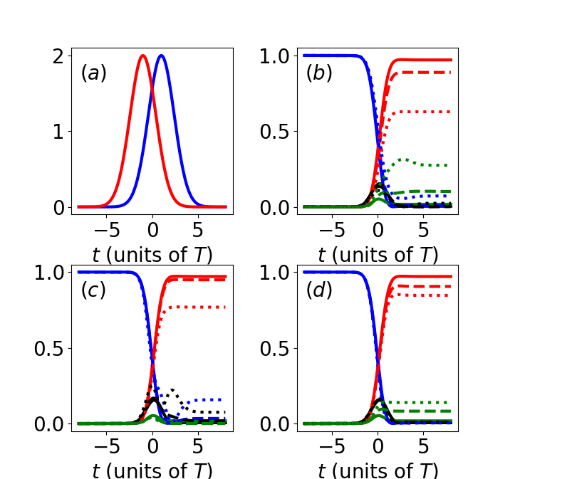
Figure 2: (a) $\Omega_{P}(t)$ and $\Omega_{S}(t)$ as functions of time $t$. In (b), (c), (d), the evolution of $\mathcal{F}_{1}(t)$ (blue lines) and $\mathcal{F}_{2}(t)$ (red lines), as well as the population left in the two bosonic modes (black lines) and in the continuum (green lines) are plotted as a function of time. (b) We fix $\gamma=0$, $\Delta=0$, $\eta_{1}=1.5$. The solid, dashed and dotted lines correspond to $\eta_{2}=1.5,1,0.5$ respectively. (c) We fix $\gamma=0$, $\eta_{1}=\eta_{2}=1.5$. The solid, dashed and dotted lines correspond to $\Delta=0,5,10$ respectively. (d) We fix $\Delta=0$, $\eta_{1}=\eta_{2}=1.5$. The solid, dashed and dotted lines correspond to $\gamma=0,0.5,1.5$ respectively. The other parameters used are $g=10$, $\Omega=2$, $\omega_{c}=2$, $T=2$.

We numerically study the quantum master equation of Eq.(4). To numerically treat the bosonic continuum, we discretize it linearly with a discretization step size $\delta$, following de Vega et al. (2015). The continuum becomes a discrete set of harmonic oscillators

$$\int_{\omega}d\omega\omega\hat{b}^{\dagger}(\omega)\hat{b}(\omega)\rightarrow\sum_{j=1}^{N}\omega_{j}\hat{b}^{\dagger}_{j}\hat{b}_{j},$$ (11)

where $N=\omega_{c}/\delta$, $\omega_{j}=j\delta$, $\hat{b}_{j}=\hat{b}(j\delta)$ and $\hat{b}^{\dagger}_{j}=\hat{b}^{\dagger}(j\delta)$. The coupling between the bosonic modes and the continuum becomes

$$\int_{\omega}d\omega\sqrt{J_{1}(\omega)}\left(\hat{a}_{1}\hat{b}^{\dagger}(\omega)+\hat{a}^{\dagger}_{1}\hat{b}(\omega)\right)\rightarrow\sum_{j=1}^{N}g_{1,j}\left(\hat{a}_{1}\hat{b}^{\dagger}_{j}+\hat{a}^{\dagger}_{1}\hat{b}_{j}\right)$$ (12)

$$\int_{\omega}d\omega\sqrt{J_{2}(\omega)}\left(\hat{a}_{2}\hat{b}^{\dagger}(\omega)+\hat{a}^{\dagger}_{2}\hat{b}(\omega)\right)\rightarrow\sum_{j=1}^{N}g_{2,j}\left(\hat{a}_{2}\hat{b}^{\dagger}_{j}+\hat{a}^{\dagger}_{2}\hat{b}_{j}\right),$$ (13)

where the discretized coupling $g_{1,j}=\sqrt{J_{1}(j\delta)\delta}$, $g_{2,j}=\sqrt{J_{2}(j\delta)\delta}$. Combining the above equations, the discretized Hamiltonian is

$$\hat{H}^{{\rm dis}}(t)= \frac{\Delta}{2}\hat{\sigma}^{z}_{1}+\frac{\Delta}{2}\hat{\sigma}^{z}_{2}+\Delta\hat{a}^{\dagger}_{1}\hat{a}_{1}+\Delta\hat{a}^{\dagger}_{2}\hat{a}_{2}+$$

$$\Omega_{P}(t)(\hat{a}^{\dagger}_{1}\hat{\sigma}^{-}_{1}+\hat{a}_{1}\hat{\sigma}^{+}_{1})+\Omega_{S}(t)(\hat{a}^{\dagger}_{2}\hat{\sigma}^{-}_{2}+\hat{a}_{2}\hat{\sigma}^{+}_{2})+$$

$$\sum_{j=1}^{N}\omega_{j}\hat{b}^{\dagger}_{j}\hat{b}_{j}+\sum_{j=1}^{N}g_{1,j}\left(\hat{a}_{1}\hat{b}^{\dagger}_{j}+\hat{a}^{\dagger}_{1}\hat{b}_{j}\right)+$$

$$\sum_{j=1}^{N}g_{2,j}\left(\hat{a}_{2}\hat{b}^{\dagger}_{j}+\hat{a}^{\dagger}_{2}\hat{b}_{j}\right).$$ (14)

In the limit $N\rightarrow\infty$, $\hat{H}^{{\rm dis}}(t)$ is equivalent to $\hat{H}(t)$ Bulla et al. (2008); de Vega et al. (2015). The discretized dissipator can be simply written as

$$\mathcal{D}^{{\rm dis}}(\hat{\rho}(t))=\gamma\sum_{j=1}^{N}\left[2\hat{b}_{j}\hat{\rho}\hat{b}^{\dagger}_{j}-\{\hat{b}^{\dagger}_{j}\hat{b}_{j},\hat{\rho}\}\right].$$ (15)

We note that $\mathcal{F}_{1}(t)$ and $\mathcal{F}_{2}(t)$ should be independent of $\delta$ as long as $\delta$ is small enough. When $\gamma=0$, we directly solve the unitary dynamics with the time dependent Hamiltonian as in Eq.(III). In case $\gamma>0$, we solve the quantum master equation in Eq.(4) with the discretized Hamiltonian as in Eq.(III) and the discretized dissipator as in Eq.(15). Although our model contains a large number of modes due to the continuum, it can be efficient solved by taking into account the fact that the model only contains at most $1$ excitation as can be seen from Eq.(6), thus we only need to consider the vacuum sector together with the single excitation sector.

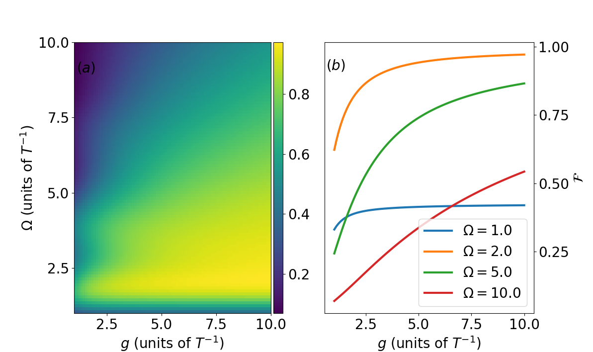
Figure 3: (a) $\mathcal{F}$ as a function of $\Omega$ and $g$. (b) Horizontal cuts of (a) for $\Omega=1,2,5,10$ respectively. Other parameters used are $\Delta=0$, $\eta_{1}=\eta_{2}=1.5$, $\gamma=0$, $T=2$, $\tau=1$, $\omega_{c}=2$.

We consider that the two couplings of laser pulses ($\Omega_{P}$ and $\Omega_{S}$) have Gaussian shapes as follows

$$\Omega_{P}(t)=\Omega\exp\left(\dfrac{-\left(t-\tau/2\right)^{2}}{T^{2}}\right),$$

$$\Omega_{S}(t)=\Omega\exp\left(\dfrac{-\left(t+\tau/2\right)^{2}}{T^{2}}\right);$$ (16)

where the $T$ is the totally time for the control process, and $\Omega$ is the maximum strength of the coupling, $\tau$ is the time delay between two pulses. $\Omega_{P}(t)$ and $\Omega_{S}(t)$ are shown in Fig. 2(a).

Figure 4: (a) $\mathcal{F}$ as a function of $\Omega$ and $\tau$, with maximum coupling strengths of laser pulses $\Omega$ from 1 $T^{-1}$ to 10 $T^{-1}$ and $\tau$ from 0.5 $T$ to 4 $T$, at fixed time $2T$. (b) $\mathcal{F}$ as a function of $\tau$ and $T$, with $\tau$ from 0.5 $T$ to 4 $T$ and totally controlling time from 1 $T$ to 5 $T$, at fixed $\Omega=2T^{-1}$.

In Fig. 2(b), we consider the effect of asymmetric couplings between the two modes $\hat{a}_{1}$, $\hat{a}_{2}$ and the continuum, namely, $J_{1}(\omega)\neq J_{2}(\omega)$. We fix $\eta_{1}=1.5$, and tune $\eta_{2}$ to be $1.5,1,0.5$. We can see that $\mathcal{F}$ is the largest when $\eta_{1}=\eta_{2}$, and decrease substantially when $\eta_{2}=0.5$, where $J_{1}(\omega)$ is super-ohmic while $J_{2}(\omega)$ is sub-ohmic, with a large portion of the population left in the continuum. It is shown in Vitanov and Stenholm (1999) that when $J_{1}(\omega)$ and $J_{2}(\omega)$ are proportional to each other, complete population transfer could be achieved. Here we show numerically that when the couplings are asymmetric, the efficiency of population transfer could be greatly reduced. In Fig.2(c), we plot the evolution of the population of the two spins with $t$ against different values of $\Delta$, namely $\Delta=0,5,10$. We can see that $\mathcal{F}$ greatly decreases when $\Delta$ is much larger than $\omega_{c}$, and a large portion of the population is left in the bosonic modes instead of the continuum in comparison with the previous case. This is because the spins are off resonant with the continuum and the population transfer is much harder (population transfer is still possible when $\Delta>\omega_{c}$ because of the strong coupling between the bosonic modes and the continuum). In Fig.2(d), we show $\mathcal{F}$ against different particle loss rate, namely $\gamma=0$ (solid line), $\gamma=0.5$ (dashed line) and $\gamma=1$ (dotted line). As expected, population transfer becomes less efficient as $\gamma$ increases.

In Fig. 3, we study the effect of the competition between the two coupling strengths $\Omega$ and $g$ on the efficiency of the population transfer. In Fig. 3(a), we plot $\mathcal{F}$ as a function of the $\Omega$ and $g$. We can see that when $\Omega\ll g$, efficient population transfer could be achieved, namely $\mathcal{F}\approx 1$. To see this more clearly, in Fig. 3(b), we plot horizontal cuts of Fig. 3(a) at different values of $\Omega$, namely $\Omega=1,2,5,10$.

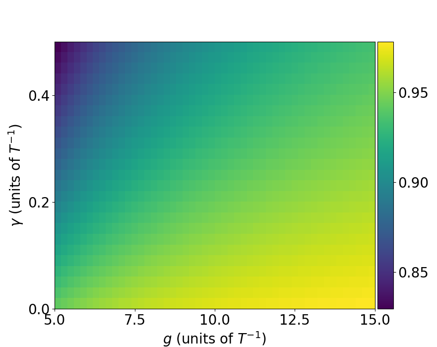
Figure 5: The $\mathcal{F}$ as a function of $g$ (coupling strengths between two qubits and spin bath) and dissipation loss $\gamma$.

Now we consider the robustness of our straddle STIRAP against the control parameters $T$, $\Omega$ and $\tau$ of laser pulses $\Omega_{P}(t)$, $\Omega_{S}(t)$, which is shown in Fig. 4. In Fig. 4(a), we shown the dependency of $\mathcal{F}$ as a function of $\Omega$ and $\tau$, where we can see that population transfer can still be achieved with high efficiency if the values of $\Omega$ and $\tau$ has small fluctuations. In Fig. 4(b), we can see that for fixed $\Omega=2$, and $\tau\approx 1$, population transfer is highly efficient for a very wide range of $T$. We also notice that for small values of $\tau$, namely $\tau\approx 0.5$, there are some oscillations for certain values of $\Omega$ and $T$. A possible reason for these oscillations is that when $\tau$ is small, the evolution is non-adiabatic, and for certain special values of $\Omega$ and $T$, some non-adiabatic shortcuts lead to similar results as the adiabatic evolution.

Finally, we study the effect of dissipation on the straddle STIRAP. We assume the bosonic continuum has a constant particle loss rate $\gamma$. In Fig. 5, we plot the dependency of $\mathcal{F}$ as a function of the particle loss rate $\gamma$ and the coupling strength $g$ between the modes $\hat{a}_{1}$, $\hat{a}_{2}$ with the continuum. We can see that as long as the coupling strength $g$ is large enough $g\geq 10$, efficient population transfer can still be achieved with moderate dissipation $\gamma\leq 1$.

IV conclusion

We propose a model to study population transfer where the intermediate states is a bosonic continuum. The model consists of two spins which are coupled to two bosonic modes with a dynamical coupling strength $\Omega_{P}(t)$ and $\Omega_{S}(t)$, and the two bosonic modes are indirectly coupled through a bosonic continuum. We show the effects on the efficiency of population transfer when tuning the the coupling strength between the bosonic modes with the continuum, as well as the various control parameters of the laser pulses. We also consider the case that when the continuum subject to a constant particle loss rate, and show that efficient population transfer can still be achieved with a moderate dissipation. We believe that this finding will be improve the high efficient transfer information in quantum information processing in future.

V Acknowledgement

We thanks the useful discussions with Prof. Tim Byrnes (Shanghai NYU) and Prof. Jonathan P. Dowling (Louisiana State University).

This work is acknowledged for funding National Science and Technology Major Project (grant no. 2017ZX02101007-003); National Natural Science Foundation of China (grant no. 61565004; 6166500; 61965005); the Natural Science Foundation of Guangxi Province (Nos. 2017GXNSFBA198116 and 2018GXNSFAA281163); the Science and Technology Program of Guangxi Province (No. 2018AD19058). W.H. is acknowledged for funding from Guangxi oversea 100 talent project and W.Z. is acknowledged for funding from Guangxi distinguished expert project.

References

- Kuklinski et al. (1989) J. Kuklinski, U. Gaubatz, F. T. Hioe, and K. Bergmann, Physical Review A 40, 6741 (1989).
- Bergmann et al. (1998) K. Bergmann, H. Theuer, and B. Shore, Reviews of Modern Physics 70, 1003 (1998).
- Huang et al. (2017) W. Huang, B. W. Shore, A. Rangelov, and E. Kyoseva, Optics Communications 382, 196 (2017).
- Falci et al. (2017) G. Falci, P. Di Stefano, A. Ridolfo, A. D’Arrigo, G. Paraoanu, and E. Paladino, Fortschritte der Physik 65, 1600077 (2017).
- Chen et al. (2018) Y.-H. Chen, Z.-C. Shi, J. Song, Y. Xia, and S.-B. Zheng, Annalen der Physik 530, 1700351 (2018).
- Kumar et al. (2016) K. Kumar, A. Vepsäläinen, S. Danilin, and G. Paraoanu, Nature communications 7, 10628 (2016).
- Helm et al. (2018) J. L. Helm, T. P. Billam, A. Rakonjac, S. L. Cornish, and S. A. Gardiner, Physical review letters 120, 063201 (2018).
- Chakraborty et al. (2017) T. Chakraborty, J. Zhang, and D. Suter, New Journal of Physics 19, 073030 (2017).
- Dory et al. (2016) C. Dory, K. A. Fischer, K. Müller, K. G. Lagoudakis, T. Sarmiento, A. Rundquist, J. L. Zhang, Y. Kelaita, and J. Vučković, Scientific reports 6, 25172 (2016).
- Huang et al. (2014) W. Huang, A. A. Rangelov, and E. Kyoseva, Physical Review A 90, 053837 (2014).
- Rangelov et al. (2011) A. Rangelov, H. Suchowski, Y. Silberberg, and N. Vitanov, Annals of Physics 326, 626 (2011).
- Dimova et al. (2015) E. Dimova, A. Rangelov, and E. Kyoseva, Journal of Optics 17, 075605 (2015).
- Huang et al. (2018a) W. Huang, S.-J. Liang, E. Kyoseva, and L. K. Ang, Semiconductor Science and Technology 33, 035014 (2018a).
- Huang et al. (2018b) W. Huang, S.-J. Liang, E. Kyoseva, and L. K. Ang, Carbon 127, 187 (2018b).
- Bergmann et al. (2019) K. Bergmann, H.-C. Nägerl, C. Panda, G. Gabrielse, E. Miloglyadov, M. Quack, G. Seyfang, G. Wichmann, S. Ospelkaus, A. Kuhn, et al., Journal of Physics B: Atomic, Molecular and Optical Physics 52, 202001 (2019).
- Vitanov et al. (2001) N. V. Vitanov, T. Halfmann, B. W. Shore, and K. Bergmann, Annual review of physical chemistry 52, 763 (2001).
- Vitanov et al. (2017) N. V. Vitanov, A. A. Rangelov, B. W. Shore, and K. Bergmann, Reviews of Modern Physics 89, 015006 (2017).
- Vitanov et al. (1998) N. Vitanov, B. W. Shore, and K. Bergmann, The European Physical Journal D-Atomic, Molecular, Optical and Plasma Physics 4, 15 (1998).
- Peters and Halfmann (2007) T. Peters and T. Halfmann, Optics communications 271, 475 (2007).
- Vitanov and Stenholm (1999) N. Vitanov and S. Stenholm, Physical Review A 60, 3820 (1999).
- Rangelov et al. (2007a) A. Rangelov, N. Vitanov, and E. Arimondo, Physical Review A 76, 043414 (2007a).
- Dreisow et al. (2009) F. Dreisow, A. Szameit, M. Heinrich, R. Keil, S. Nolte, A. Tünnermann, and S. Longhi, Optics letters 34, 2405 (2009).
- Longhi (2008) S. Longhi, Physical Review A 78, 013815 (2008).
- Rangelov et al. (2007b) A. Rangelov, N. Vitanov, and E. Arimondo, Physical Review A 76, 043414 (2007b).
- Deng et al. (2016) T. Deng, Y. Yan, L. Chen, and Y. Zhao, The Journal of chemical physics 144, 144102 (2016).
- Contreras-Pulido and Aguado (2008) L. Contreras-Pulido and R. Aguado, Physical Review B 77, 155420 (2008).
- De Vega and Alonso (2017) I. De Vega and D. Alonso, Reviews of Modern Physics 89, 015001 (2017).
- de Vega et al. (2015) I. de Vega, U. Schollwöck, and F. A. Wolf, Physical Review B 92, 155126 (2015).
- Bulla et al. (2008) R. Bulla, T. A. Costi, and T. Pruschke, Reviews of Modern Physics 80, 395 (2008).