Finite N corrections to white hot string bits

Abstract

String bit systems exhibit a Hagedorn transition in the $N\to\infty$ limit. However, there is no phase transition when $N$ is finite (but still large). We calculate two-loop, finite $N$ corrections to the partition function in the low-temperature regime. The Haar measure in the singlet-restricted partition function contributes pieces to loop corrections that diverge as $\mathcal{O}(N)$ when summed over the mode numbers. We study how these divergent pieces cancel each other out when combined. The properly normalized two-loop corrections vanish as $\mathcal{O}(N^{-1})$ for all temperatures below the Hagedorn temperature. The coefficient of this $1/N$ dependence decreases with temperature and diverges at the Hagedorn pole.

I Introduction

One can study a light-cone-quantized string as the continuum limit of a polymer of point masses called string bits Giles and Thorn (1977); Thorn (1991). These bits move in transverse space, enjoy nearest-neighbor interactions and transform adjointly under a global $U(N)$ symmetry. It is possible to incorporate target space supersymmetry Bergman and Thorn (1995) into this picture. The longitudinal coordinate is recovered in the large $N$’t Hooft (1974) limit and the continuum limit of such a polymer. In fact, as an extreme form of holography, one may recover all the coordinates (instead of simply the longitudinal one) by postulating extra internal degrees of freedom (d.o.f) Thorn (2014). It is instructive to study the behavior of such a system at finite temperature Thorn (2015); Raha (2017); Curtright et al. (2017). Such systems exhibit a Hagedorn transition from a low-temperature phase that consists of closed chains to a high-temperature phase consisting of liberated bits. This bears similarities to Hagedorn transitions studied in various other models: Hermitian matrix model Brézin et al. (1978), unitary matrix model Gross and Witten (1980) and $\mathcal{N}=4$ supersymmetric Yang-Mills (SYM) theory on $S^{3}$ Sundborg (2000); Aharony et al. (2004). For an improved calculation of Hagedorn temperature in $\mathcal{N}=4$ SYM theory at finite ’t Hooft’s coupling see Harmark and Wilhelm (2018a, b).

In a recent paper Curtright et al. (2017) we have computed the low-temperature partition function of the simplest stable string bit system, up to leading order in $N$. In that simplified model, interactions between the string bits were switched off and instead, a singlet restriction was imposed on them. In the appropriate limits, this rudimentary system corresponds to the $T_{0}\to 0$ limit of a subcritical string in $1+1$ dimensions that has only one Grassmann world sheet field. We observed that the singlet restriction can be studied as $1/N$ perturbations in an effective scalar field theory. The Hagedorn temperature of the system could then be understood as the location of the pole of the “bare propagator” in this effective field theory. At large but finite $N$ the system is not supposed to have a Hagedorn transition (there are only a finite number of (d.o.f) at finite $N$). This motivated us to do a partial resummation of the bare propagator with quartic corrections to shift the Hagedorn pole off the real temperature axis. Only at infinite temperature did we manage to compute finite $N$ corrections to the partition function and discovered its link to an enumeration problem of Eulerian digraphs with $N$ nodes. As a follow-up to our paper, Beccaria used the technique developed in Aharony et al. (2004) to calculate the density of eigenvalues in the high-temperature phase up to leading order in $N$ Beccaria (2017).

In this paper we shall present finite $N$ corrections to the following partition function in the low-temperature regime:

$$Z=\dfrac{\left(\dfrac{1+x}{1-x}\right)^{N-1}\left(\displaystyle\int^{\pi}_{-\pi}\displaystyle\prod_{k=1}^{N}d\theta_{k}\right)\left(\displaystyle\prod_{1\leq i<j\leq N}4\sin^{2}\left(\dfrac{\theta_{i}-\theta_{j}}{2}\right)\dfrac{|1+xe^{i(\theta_{i}-\theta_{j})}|^{2f}}{|1-xe^{i(\theta_{i}-\theta_{j})}|^{2b}}\right)}{\left(\displaystyle\int^{\pi}_{-\pi}\displaystyle\prod_{k=1}^{N}d\theta_{k}\right)\left(\displaystyle\prod_{1\leq i<j\leq N}4\sin^{2}\left(\dfrac{\theta_{i}-\theta_{j}}{2}\right)\right)}$$ (1)

where $x=e^{-\beta\omega}$, $\theta_{k}$ represents the $k$th angle in the $U(N)$ color space $\forall k\in\{1,N\}$, $b$ is the number of distinct bosonic species and $f$ is the number of distinct fermionic species in the system. $\beta$ denotes $\dfrac{1}{k_{B}T}$ and $\omega$ denotes the mass of a string bit. Our results will hold for $0\leqslant x<\dfrac{1}{b+f}$. The connected vacuum diagrams are then represented by

$$\log(Z)=\log\int^{\pi}_{-\pi}\prod^{N}_{k=1}d\theta_{k}\exp[L(x;\{\theta\})]-\log\int^{\pi}_{-\pi}\prod^{N}_{k=1}d\theta_{k}\exp[L(0;\{\theta\})]$$ (2)

where

$$L(x;\{\theta\})=(N-1)\log\left(\dfrac{1+x}{1-x}\right)+\dfrac{1}{2}\sum_{i\neq j}\mathcal{L}(x;\theta_{i}-\theta_{j})$$ (3)

with

$$\mathcal{L}(x;\theta)=\log(1-e^{i\theta})+f\log(1+xe^{i\theta})-b\log(1-xe^{i\theta})+c.c.$$ (4)

containing pieces from the group measure, fermionic bits and bosonic bits, respectively. In the low-temperature phase, $L$ is maximized by a uniform distribution, $\theta_{0}$, of $\{\theta\}$. One can take a nondecreasing function of the indices,

$${\theta_{0_{k}}} =2\pi\dfrac{k}{N} k \in\{1,\ldots,N\}$$ (5)

and expand this effective Lagrangian about this uniform distribution. Then using perturbation theory for scalar field

$$\log\left(\int e^{L}\right)=L_{0}+\frac{1}{2}\log\left(\det\left[\dfrac{2\pi}{-L_{2}}\right]\right)+\left.\log\left[\exp\left\{\dfrac{L_{3}}{3!}\left(\dfrac{\delta}{\delta J}\right)^{3}+\dfrac{L_{4}}{4!}\left(\dfrac{\delta}{\delta J}\right)^{4}+\cdots\right\}\exp\left\{\dfrac{J^{2}}{2(-L_{2})}\right\}\right]\right|_{J=0}\\ \approx L_{0}+\frac{1}{2}\log\left(\det\left[\dfrac{2\pi}{-L_{2}}\right]\right)-\dfrac{1}{12}\sum_{m,n}\dfrac{V_{m,n,-m-n}V_{-m,-n,m+n}}{V_{m,-m}V_{n,-n}V_{-m-n,m+n}}+\frac{1}{8}\sum_{m,n}\dfrac{V_{m,-m,n,-n}}{V_{m,-m}V_{n,-n}}+\cdots$$ (6)

where $L_{p}\equiv L_{k_{1},\ldots,k_{p}}=\dfrac{\delta^{p}L[\theta_{0}]}{\delta\theta_{k_{1}}\cdots\delta\theta_{k_{p}}}$ are the coupling constants in “position space” and

$$V_{n_{1},\ldots,n_{p}}=\dfrac{1}{N^{p/2}}\sum^{N}_{k_{1},\cdots,k_{p}=1}L_{k_{1},\ldots,k_{p}}e^{2\pi i(n_{1}k_{1}+\cdots+n_{p}k_{p})/N}$$ (7)

are the coupling constants in “Fourier space.” $L_{2}[\theta_{0}]$ turns out to be a circulant matrix in the “position indices,” i.e. $L_{m,n}[\theta_{0}]=F(|m-n|)$, and hence can be naturally diagonalized via the Fourier transform Curtright et al. (2017).

II Calculation of vertices for finite $N$

In Curtright et al. (2017), the $p$th Fourier vertex is given by

$$V_{n_{1}\cdots n_{p}}=\frac{\delta_{N|n_{1}+\cdots+n_{p}}}{2N^{1-p/2}}\sum^{N-1}_{\alpha=1}\frac{d^{p}\mathcal{L}\left(2\pi\dfrac{\alpha}{N}\right)}{d\theta^{p}}(e^{2\pi i\alpha n_{1}/N}-1)\cdots(e^{2\pi i\alpha n_{p}/N}-1)$$ (8)

where $n_{l}\in\mathbb{Z}\forall l\in\{1,p\}$ represents the Fourier mode numbers, and the delta symbol is $1$ whenever $N$ is a factor of $n_{1}+\cdots+n_{p}$ and $0$ otherwise. $\mathcal{L}$ is a function of differences in $\theta$’s, hence its derivative with respect to a single $\theta_{k}$ yields differences in Kronecker deltas:

$$\dfrac{d\mathcal{L}}{d\theta_{k}}=\sum_{i\neq j}(\delta_{ik}-\delta_{jk})\mathcal{L}^{\prime}(\theta_{k})$$ (9)

Upon a Fourier transform these differences in Kronecker deltas yield products of differences between powers of roots of unity:$(e^{2\pi i\alpha n_{1}/N}-e^{2\pi i\beta n_{1}/N})\cdots(e^{2\pi i\alpha n_{p}/N}-e^{2\pi i\beta n_{p}/N})$. Following this, in Curtright et al. (2017) we approximated the sum over $\alpha$ by an integral. In this paper, we shall perform the exact summation.

But first, let us try to evaluate the following expression

$$\mathcal{B}(\{n\};t)=\sum_{\alpha}\left.(e^{in_{1}\theta_{\alpha}}-1)\cdots(e^{in_{p}\theta_{\alpha}}-1)\left(\dfrac{d}{d\theta_{\alpha}}\right)^{p}\log(1-e^{t+i\theta_{\alpha}})\right|_{\theta_{k}=2\pi\tfrac{k}{N}}\\ =\left(i\dfrac{d}{dt}\right)^{p}\sum_{\alpha}(e^{2\pi in_{1}\alpha/N}-1)\cdots(e^{2\pi in_{p}\alpha/N}-1)\log(1-e^{t+2\pi i\alpha/N})$$ (10)

where $\{n\}\equiv\{n_{1},\cdots,n_{p}\}$ and in the first line we are evaluating the entire summand at uniform distribution, $\theta_{0}$. The derivative with respect to any $\theta_{\alpha}$ can be replaced by $i\dfrac{d}{dt}$ . This enables one to pull the derivative operator outside the sum. This leaves the sum to be independent of the order, $p$, of the vertex. One can generate any vertex by repeatedly applying $i\dfrac{d}{dt}$ on this universal sum. Expanding the logarithm on rhs we get

$$\mathcal{B}(\{n\};t)=-\left(i\dfrac{d}{dt}\right)^{p}\sum_{m=1}^{\infty}\dfrac{e^{mt}}{m}\sum_{\alpha=1}^{N-1}e^{2\pi im\alpha/N}(e^{2\pi in_{1}\alpha/N}-1)\cdots(e^{2\pi in_{p}\alpha/N}-1)\\ =-i^{p}\left(\dfrac{d}{dt}\right)^{p-1}\sum_{m=1}^{\infty}e^{mt}\sum_{\alpha=1}^{N-1}\sum_{s\in\{n\}}C_{y(s)}e^{2\pi i(m+\widetilde{y(s)})\alpha/N}$$ (11)

where,

$$(e^{2\pi in_{1}\alpha/N}-1)\cdots(e^{2\pi in_{p}\alpha/N}-1)=\sum_{s\in\{n\}}C_{y(s)}e^{2\pi i\widetilde{y(s)}\alpha/N}$$ (12)

with $y(s)$ denoting the sum total of the elements in a subset $s$ of $\{n\}$. For example, $y(s)$ could represent $(n_{1}+n_{5})$ , $(n_{2}+n_{3}+n_{p-1})$, etc. $C_{y(s)}\in\{-1,+1\}$ is the coefficient corresponding to a particular $s$ and $\widetilde{y(s)}\equiv y(s)\mod N$. The sum over $s$ represents a sum over all possible ways of obtaining subsets from $\{n\}$. Finally, we have

$$\mathcal{B}(\{n\};t)=-i^{p}\left(\dfrac{d}{dt}\right)^{p-1}\sum_{s\in\{n\}}C_{y(s)}\left\{\dfrac{Ne^{t(N-\widetilde{y(s)})}}{1-e^{tN}}-\dfrac{e^{t}}{1-e^{t}}\right\}$$ (13)

The presence of the mod function (represented by $\widetilde{\ }$ ) tells one that $\mathcal{B}(\{n\};t)$ is periodic in each value of $n$. Now one can express $V$’s in a very compact form in terms of these $\mathcal{B}$’s:

$$V_{n_{1},\cdots,n_{p}}=\frac{\delta_{N|n_{1}+\cdots+n_{p}}}{2N^{1-p/2}}\left\{\displaystyle\lim_{t\rightarrow 0^{-}}\mathcal{B}(\{n\};t)+\displaystyle\lim_{t\rightarrow 0^{-}}\mathcal{B}(\{-n\};t)^{\ast}\\ +f\mathcal{B}\left(\{n\};-\beta\omega+i\pi\right)+f\mathcal{B}(\{-n\};-\beta\omega+i\pi)^{\ast}\\ -b\mathcal{B}(\{n\};-\beta\omega)-b\mathcal{B}(\{-n\};-\beta\omega)^{\ast}\right\}$$ (14)

where $\{-n\}\equiv\{-n_{1},\cdots,-n_{p}\}$ and “^∗” denotes complex conjugation.

This is the formula with which we may compute any diagram at finite $N$. In a parallel to Eq. [4], one can verify that the terms in the first row account for the contribution from the group measure, the second row accounts for the adjoint fermions and the third row for the adjoint bosons. The (bare) inverse propagator then is given by

$$V_{n,N-n}=\left\{N^{2}\left(b\dfrac{(1-x^{n})^{2}x^{N-n}}{(1-x^{N})^{2}}-f\dfrac{(1-(-x)^{n})^{2}(-x)^{N-n}}{(1-(-x)^{N})^{2}}\right)-Nn\left(b\dfrac{x^{n}-x^{N-n}}{1-x^{N}}-f\dfrac{(-x)^{n}-(-x)^{N-n}}{1-(-x)^{N}}+1\right)+n^{2}\right\}$$ (15)

where $N>n>0$. With some inspection one can confirm that the rhs of this equation is symmetric under the interchange of $n\leftrightarrow N-n$. With finite $n$, as $N\rightarrow\infty$,

$$V_{n,N-n}\approx-Nn\{1-bx^{n}+f(-x)^{n}\}=-NnI_{n}$$ (16)

which reproduces the (leading order in $N$) result obtained in Curtright et al. (2017), with $I_{n}$ denoting the temperature dependent factor.

At $x=0$ (zero temperature) Eq. [15] gives $V_{n,N-n}=n(n-N)$. Physically, this signifies the (bare) inverse propagator when the integrand in

$$\mathcal{I}=\int_{-\pi}^{\pi}\prod_{k=1}^{N}d\theta_{k}\prod_{i<j}4\sin^{2}\left(\dfrac{\theta_{i}-\theta_{j}}{2}\right)$$ (17)

is expanded about the $\theta_{0}$ (the uniform distribution, also the global maximum). $\mathcal{I}$ is the same as the normalization on the rhs of Eq. [1]. Using the method of steepest descent, one may calculate this integral to be

$$\mathcal{I}=N!\exp\left\{N\log(N)+\log(2\pi)+\dfrac{N-1}{2}\log(2\pi)-\log((N-1)!)+\Lambda\right\}$$ (18)

where the prefactor is due to the permutation symmetry of the integrand under the exchange of $i,j$ indices. The first term in the parentheses indicates the value of the integrand at uniform distribution while the next three terms come from Gaussian fluctuations about the uniform distribution. However, $\mathcal{I}$ can be computed exactly and is known to be equal to $N!(2\pi)^{N}$. We can use the known answer to estimate the asymptotics of the higher order (i.e. beyond Gaussian) corrections,

$$\Lambda=-N\log(N)+\dfrac{N-1}{2}\log(2\pi)+\log((N-1)!)=-\left(1-\dfrac{\log(2\pi)}{2}\right)N-\dfrac{1}{2}\log(N)+\cdots$$ (19)

This shows that Gaussian fluctuations are not enough to approximate $\mathcal{I}$ as $N\rightarrow\infty$. We can numerically show that one needs to take into account at least the two-loop corrections in order to obtain the correct (large $N$) limit.

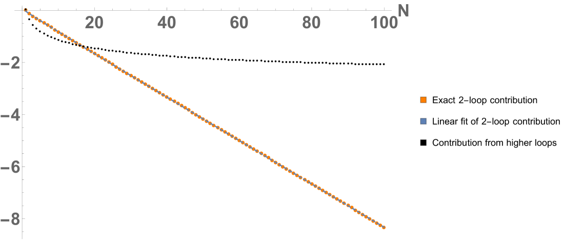
Figure 1: Contribution of loop diagrams to the log of the integral of the Haar measure, shown as a function of $N$. Two-loop corrections seem to account for the linear divergence of beyond-Gaussian contributions. The slope of the linear fit to the two-loop contribution is $-0.08297\pm 0.00003$.

Fig. [1] tells us that the two-loop diagrams contribute up to $\mathcal{O}(N)$ to the integral in Eq. [17]. The higher-loop diagrams seem to contribute only up to subleading $\mathcal{O}(\log(N))$ corrections. However, the numerical error in estimating the slope is too small. That is, even though the diagram may suggest otherwise, higher-loop diagrams do have a minuscule contribution to the linear divergence. Coming back to Eq. [1], one cannot rule out a similar thing from happening to $\log(Z)$ either. This integral, too, may end up with beyond-Gaussian corrections that consist of pieces that diverge for large $N$. This would, in turn, challenge our assumption Raha (2017); Curtright et al. (2017) that stopping at Gaussian fluctuations is enough to accurately compute large $N$ behavior of $\log(Z)$. At this point one may think of normalization in the definition of Eq. [1] and expect it to remove these potential divergences at loop order. However, one cannot be sure of such a cancellation a priori. One can analyze e.g., the double-cubic term on the rhs of Eq. [6] to see why. If each vertex had a divergent component of a certain order, a rational function of these vertices (which is what a Feynman diagram is) would give rise to new divergences. One can expect normalization to remove the leading divergence in such a function. But divergences of next-to-leading order, arising from the “cross terms” in the Feynman diagram, could still be left unaltered. To the best of our knowledge, one cannot guarantee the cancellation of these subleading divergences in an arbitrary Lagrangian. The fate of these divergences has to be found out by explicitly computing the 2-loop corrections. Thus we are motivated to calculate corrections to $\log(Z)$ up to two-loop order in the following section.

III Two-loop Corrections

Like the (bare) inverse propagator in the previous section, one can compute any (bare) vertex for finite values of $N$. For two-loop corrections one needs expressions for the cubic and the quartic vertices only. There is no contribution of the two-loop “dumbbell” diagram; as we see in Curtright et al. (2017) that $V_{n,-n,0}$ vanishes for our system. The only contributions are from the “theta” (double-cubic) and the “infinity” (quartic) diagrams (see Fig. [2]).

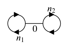
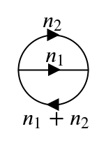
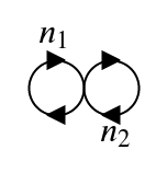
Figure 2: The possible two-loop corrections to the Gaussian result. In the system under consideration, the dumbbell diagram does not contribute.

III.1 Cubic contribution

The cubic vertex, using Eq. [14], is represented by

$$V_{n_{1},n_{2},-n_{1}-n_{2}}=\left\{b\sqrt{N}i\left(N^{2}(1+x^{N})\frac{\left(x^{N-(\widetilde{-n_{1}})}-x^{N-\widetilde{n_{1}}}\right)}{(1-x^{N})^{3}}-2N\frac{(\widetilde{-n_{1}})x^{N-(\widetilde{-n_{1}})}-\widetilde{n_{1}}x^{N-\widetilde{n_{1}}}}{(1-x^{N})^{2}}+\frac{(\widetilde{-n_{1}})^{2}x^{N-(\widetilde{-n_{1}})}-(\widetilde{n_{1}})^{2}x^{N-\widetilde{n_{1}}}}{1-x^{N}}\right)\\ +{\color[rgb]{0,0,1}{\{b\rightarrow-f,x\rightarrow-x\}}}\\ -\frac{i}{6\sqrt{N}}\left(N^{2}\text{}\left(\left(\widetilde{-n_{1}}\right)-\widetilde{n_{1}}\right)-3N((\widetilde{-n_{1}})^{2}-(\widetilde{n_{1}})^{2})+2((\widetilde{-n_{1}})^{3}-(\widetilde{n_{1}})^{3})\right)\\ +{\color[rgb]{0,0,1}{\{n_{1}\rightarrow n_{2}\}}}+{\color[rgb]{0,0,1}{\{n_{1}\rightarrow-n_{1}-n_{2}\}}}\right\}$$ (20)

Here the third line on the rhs indicates that the fermionic contribution is obtained by making corresponding substitutions in all the lines above it. Similarly, the fifth line indicates that one obtains two more copies by making the suggested substitutions in all the lines preceding it. Besides the explicit symmetry under the permutations of the indices, one can see that the rhs is an odd function of the indices. In other words

$$V_{-n_{1},-n_{2},n_{1}+n_{2}}=-V_{n_{1},n_{2},-n_{1}-n_{2}}=V_{n_{1},n_{2},-n_{1}-n_{2}}^{\ast}$$ (21)

The contribution of the theta diagram is given by

$$\Lambda_{3}=-\dfrac{1}{12}\sum_{n_{1},n_{2}=1}^{N}\left(\dfrac{V_{n_{1},n_{2},-n_{1}-n_{2}}V_{-n_{1},-n_{2},n_{1}+n_{2}}}{V_{n_{1},-n_{1}}V_{n_{2},-n_{2}}V_{-n_{1}-n_{2},n_{1}+n_{2}}}-{\color[rgb]{0,0,1}{\{x\rightarrow 0\}}}\right)$$ (22)

where the subtracted part ensures proper, order-by-order normalization of the diagram. An order-by-order normalization implies that one is expanding the denominator on the rhs of Eq. [1) about the uniform distribution as well. This ensures the correct normalization of $Z$, i.e. at $x=0$, $Z$ will equal $1$ up to any order in perturbation. An expansion of the summand of $\Lambda_{3}$ is neither compact nor illuminating. It is far more useful to see it graphically

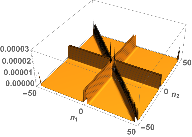
Figure 3: Dependence on loop momenta $n_{1}$ & $n_{2}$ of the summand of the cubic two-loop diagram for $N=100$, $x=0.125$, $b=f=1$. The discontinuities represent regions where the propagators vanish, i.e. the zero modes.

Fig. [3] indicates that the double summation over loop momenta yields an extra factor of $N$. One can deduce this from the presence of ridge lines along $n_{1},n_{2}\approx\pm 1$. The ridges have constant (nonzero) height and width, which leads to an extra factor of $N$ upon summation. While it would be desirable to obtain a closed-form expression for $\Lambda_{3}$, one can nonetheless employ numerics to study its behavior. Fig.[4] is what one gets as one proceeds to actually plot the contribution of this diagram (after summing over all the modes). This plot suggests that the summand of $\Lambda_{3}$ is $\mathcal{O}(N^{-2})$. That way, $\Lambda_{3}$ can vanish as $\dfrac{1}{N}$, despite an extra factor of $N$ produced after the sum over modes.

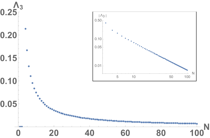
Figure 4: Dependence on $N$ of the two-loop double-cubic corrections to the log of the partition function at $x=0.125$ for $b=f=1$. The inset displays the log-log scaled version of the main plot and has a slope of $-1.057\pm 0.005$. This indicates that $\Lambda_{3}\sim\mathcal{O}(N^{-1})$.

III.2 Quartic contribution

Similarly, using Eq. [14] for the quartic vertex one obtains:

$$V_{n_{1},n_{2},-n_{1},-n_{2}}=\left\{2b\left(-N^{3}(1+4x^{N}+x^{2N})\dfrac{x^{N-(\widetilde{-n_{1}})}+x^{N-\widetilde{n_{1}}}}{(1-x^{N})^{4}}+3N^{2}(1+x^{N})\frac{(\widetilde{-n_{1}})x^{N-(\widetilde{-n_{1}})}+\widetilde{n_{1}}x^{N-\widetilde{n_{1}}}}{(1-x^{N})^{3}}-3N\frac{(\widetilde{-n_{1}})^{2}x^{N-(\widetilde{-n_{1}})}+(\widetilde{n_{1}})^{2}x^{N-\widetilde{n_{1}}}}{(1-x^{N})^{2}}+\frac{(\widetilde{-n_{1}})^{3}x^{N-(\widetilde{-n_{1}})}+(\widetilde{n_{1}})^{3}x^{N-\widetilde{n_{1}}}}{1-x^{N}}\right)\\ +{\color[rgb]{0,0,1}{\{b\rightarrow-f,x\rightarrow-x\}}}\\ -N\dfrac{(\widetilde{-n_{1}})^{2}+(\widetilde{n_{1}})^{2}}{2}+(\widetilde{-n_{1}})^{3}+(\widetilde{n_{1}})^{3}-\dfrac{\text{}(\widetilde{-n_{1}})^{4}+(\widetilde{n_{1}})^{4}}{2N}\\ +{\color[rgb]{0,0,1}{\{n_{1}\rightarrow n_{2}\}}}-\dfrac{1}{2}{\color[rgb]{0,0,1}{\{n_{1}\rightarrow n_{1}+n_{2}\}}}-\frac{1}{2}{\color[rgb]{0,0,1}{\{n_{1}\rightarrow n_{1}-n_{2}\}}}\\ +4N^{3}\left(\dfrac{bx^{N}(1+4x^{N}+x^{2N})}{(1-x^{N})^{4}}-\dfrac{f(-x)^{N}(1-4(-x)^{N}+x^{2N})}{(1+(-x)^{N})^{4}}\right)\right\}$$ (23)

Just like the cubic vertex, one obtains various parts by making indicated substitutions in all the lines preceding said substitution. Here, because of the symmetry under the permutations of the indices, one can see that the rhs is an even function in the indices. The contribution from quartic correction to $\log(Z)$ is given by a double sum over $n_{1}$ and $n_{2}$. It is given by

$$\Lambda_{4}=\dfrac{1}{8}\sum_{n_{1},n_{2}=1}^{N}\left(\dfrac{V_{n_{1},-n_{1},n_{2},-n_{2}}}{V_{n_{1},-n_{1}}V_{n_{2},-n_{2}}}-{\color[rgb]{0,0,1}{\{x\rightarrow 0\}}}\right)$$ (24)

again, the expression being appropriately normalized.

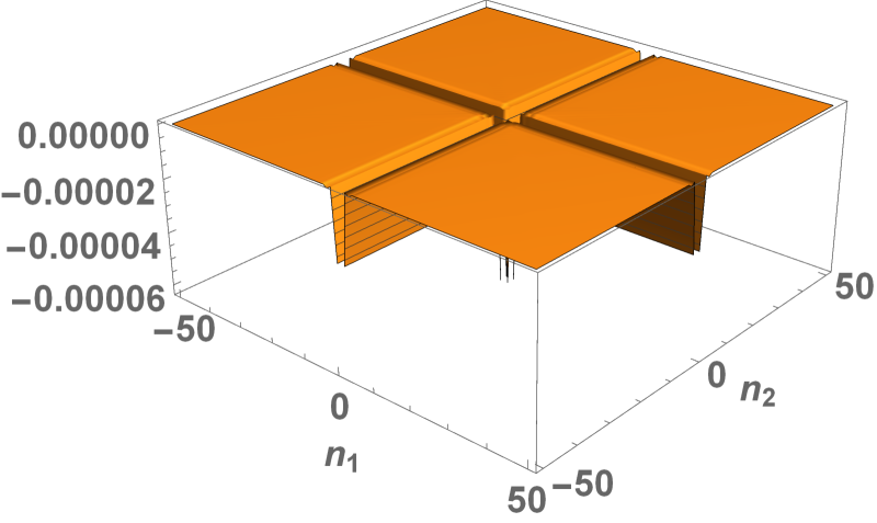
Figure 5: Dependence on loop momenta $n_{1}$ and $n_{2}$ of the summand of the quartic two-loop diagram for $N=100$, $x=0.125$, $b=f=1$. The discontinuities represent regions where the propagators vanish.

In a parallel to the previous subsection, one may examine Fig. [5] and see a factor of $N$ in it. Again, the primary contribution to the sum comes from regions that have small mode number, i.e. $|n_{1}|=|n_{2}|\approx 1$. And just like the cubic case, Fig. [6] reveals that the summand in $\Lambda_{4}$ too goes as $\mathcal{O}(N^{-2})$.

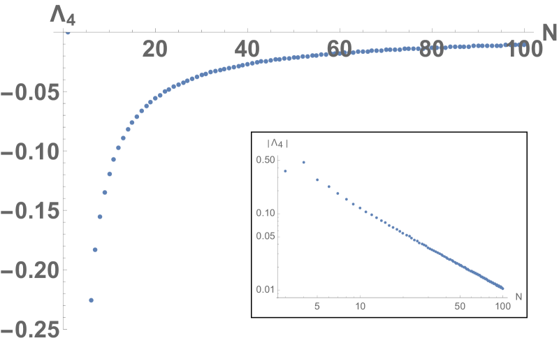
Figure 6: Dependence on $N$ of the two-loop quartic corrections to the log of the partition function at $x=0.125$ for $b=f=1$. The inset displays a log-log scaled version of the main plot and has a slope of $-1.071{\pm}0.006$. This indicates that $\Lambda_{4}\sim\mathcal{O}(N^{-1})$.

In the next section, we shall discuss the reasons for this large $N$ dependence. We shall identify pieces in the summand of each diagram that diverge on their own. And we shall try to see which pieces cancel each other out when combined.

IV Discussions

In Fig. [7] we have plotted full two-loop corrections for different values of $x$ (but each below $x_{H}$). In the low-temperature phase, one-loop corrections are already included in the infinite $N$ result, and the two-loop corrections are the leading finite $N$ corrections. One can immediately notice that the latter are negative for large enough $N$. In [Raha (2017)] we have presented exact $\log(Z)$ as analytic functions of temperature, for a few small values of $N$. At least for those cases, $\log(Z)$ seems to increase with $N$. Since $\log(Z)$ is not known as an analytic function of $N$ it is not obvious whether this trend continues for higher values of $N$. The negative sign of the (leading) finite $N$ corrections is, however, consistent with such a trend. There is obviously no phase transition in a system with finite degrees of freedom. One can see this in [Raha (2017)] where exact partition functions for small $N$ have no divergence except at infinite temperature. Because of the negative sign, the two-loop corrections assist in pushing the Hagedorn pole to a higher temperature. Including finite $N$ corrections to all loop orders would eventually push the corresponding Hagedorn temperature to infinity.

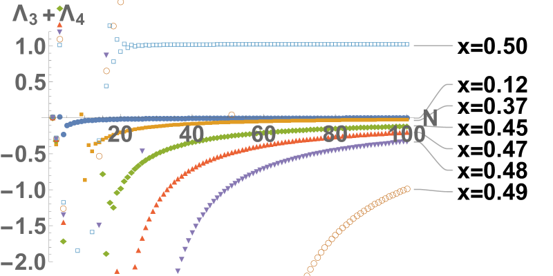
Figure 7: Full two-loop corrections to the log of the partition function at different values of $x$ for $b=f=1$ as functions of $N$. For $x<\dfrac{1}{b+f}$, the two-loop contribution is negative and vanishes as $\mathcal{O}(N^{-1})$ for large $N$.

The trend of negative values of corrections breaks down at the Hagedorn temperature. There the correction is positive and seems to be independent of $N$. Above the Hagedorn point the uniform distribution is no longer the maximizing distribution. This abrupt change indicates the onset of the high-temperature regime, where one has to obtain a new formula for the vertex $V_{n_{1},\cdots,n_{p}}$. In the low-temperature regime the finite $N$ corrections vanish as $\sim\dfrac{c(x)}{N}$. One may extract $c(x)$ by computing $\displaystyle\lim_{N\to\infty}N(\Lambda_{3}+\Lambda_{4})$. In Fig. [8] we have shown the temperature dependence of this coefficient. $c(x)$ decreases with temperature and seems to diverge at the Hagedorn temperature. A crude curve-fitting exercise indicates that for smaller temperatures

$$c(x) \approx 1-\dfrac{1}{1-2x} x \sim 0$$ (25)

However, an analysis of log-log plot near the Hagedorn point shows that the dependence of $c(x)$ on $x$ is not a simple power law.

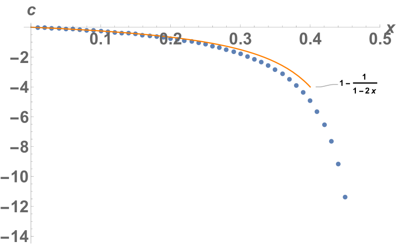
Figure 8: The coefficient of $\dfrac{1}{N}$ in the two-loop corrections as a function of temperature ($x=e^{-\frac{\omega}{k_{B}T}}$), for the case $b=f=1$. There is a divergence at the Hagedorn temperature.

In the previous section, we deduced from Figs. [3], [4], [5] & [6] that the summands of $\Lambda_{3}$ and $\Lambda_{4}$ each were $\mathcal{O}(N^{-2})$. Analyzing the cubic and quartic vertices we can see why this is so. For simpler analysis, we shall keep $n_{1}$ and $n_{2}$ finite and make $N$ large. When $N$ is large,

$$\tilde{s}\equiv s\mod N =\begin{cases}s&s\geqslant 0\\ N+s&s<0\end{cases} x^{N} \approx 0$$ (26)

Using these simplifications, the cubic vertex becomes

$$V_{n_{1},n_{2},-n_{1}-n_{2}}\approx-i\sqrt{N}\left\{n_{1}^{2}\text{sgn}(n_{1})(1-bx^{|n_{1}|}+f(-x)^{|n_{1}|})+n_{2}^{2}\text{sgn}(n_{2})\left(1-bx^{|n_{2}|}+f(-x)^{|n_{2}|}\right)\\ -(n_{1}+n_{2})^{2}\text{sgn}(n_{1}+n_{2})(1-bx^{|n_{1}+n_{2}|}+f(-x)^{|n_{1}+n_{2}|})\right\}\\ =-i\sqrt{N}\left\{n_{1}^{2}\text{sgn}(n_{1})I_{|n_{1}|}+n_{2}^{2}\text{sgn}(n_{2})I_{|n_{2}|}-(n_{1}+n_{2})^{2}\text{sgn}(n_{1}+n_{2})I_{|n_{1}+n_{2}|}\right\}$$ (27)

while the quartic vertex looks like

$$V_{n_{1},n_{2},-n_{1},-n_{2}}\approx\left\{2|n_{1}|^{3}(1-bx^{|n_{1}|}+f(-x)^{|n_{1}|})+2|n_{2}|^{3}(1-bx^{|n_{2}|}+f(-x)^{|n_{2}|})\\ -|n_{1}-n_{2}|^{3}(1-bx^{|n_{1}-n_{2}|}+f(-x)^{|n_{1}-n_{2}|})-|n_{1}+n_{2}|^{3}(1-bx^{|n_{1}+n_{2}|}+f(-x)^{|n_{1}+n_{2}|})\right\}\\ =2|n_{1}|^{3}I_{|n_{1}|}+2|n_{2}|^{3}I_{|n_{2}|}-|n_{1}-n_{2}|^{3}I_{|n_{1}-n_{2}|}-|n_{1}+n_{2}|^{3}I_{|n_{1}+n_{2}|}$$ (28)

From Eqs. [16, [27] and [28] it becomes clear that the summands on the rhs of Eqs. [22] and [24] go as $\sim\dfrac{n}{N^{2}}$. This confirms our guess regarding the asymptotic $N$ dependence of each summand.

However, this also creates a new complication. Such a dependence on $n$ should lead to an $\mathcal{O}(N)$ divergence for each of $\Lambda_{3}$ and $\Lambda_{4}$ after the double sum over mode numbers is performed. This is clearly against the numerical evidence that we have at hand. From Eqs. [22] and [24] we expect each summand to go as $\sim\dfrac{1}{N^{2}n}$ instead of the $\sim\dfrac{n}{N^{2}}$ that we see here. While normalization can be expected to remove the leading divergent pieces (the ones that go as $\sim\dfrac{n}{N^{2}}$), it is not at all clear how the subleading pieces that go as $\sim\dfrac{1}{N^{2}}$ get canceled. For that one has to take a closer look at all the pieces in $\Lambda_{3}$ and $\Lambda_{4}$. The key lies in the $I_{|n|}$’s. They come with a $1$ and exponential convergent factors: $x^{|n|}=e^{-\beta\omega|n|}$. All pieces whose numerators go as $\sim x^{|n_{1}|+|n_{2}|}$ are absolutely convergent upon the double sum over $n_{1}$ and $n_{2}$. Only the $1$ in the $I_{|n|}$ could lead to divergences. For example, pieces that have this exponential convergence in only one of the modes, i.e., pieces that go as $\sim x^{|n_{1}|}$ or $\sim x^{|n_{2}|}$, may be divergent (or convergent depending upon the power of the other mode). The worst fate is for the pieces whose numerators have no convergence factor in either $n_{1}$ or $n_{2}$. However, one must keep in mind that such pieces may ultimately get their divergences removed by proper normalization.

$\begin{array}[]{|l|}\hline\cr\dfrac{n_{1}^{3}\left(2\text{sgn}(n_{1})-\text{sgn}(n_{1}-n_{2})-\text{sgn}(n_{1}+n_{2})\right)}{8N^{2}|n_{1}||n_{2}|I_{|n_{1}|}I_{|n_{2}|}}\\ \\ \dfrac{3n_{1}^{2}n_{2}\left(\text{sgn}(n_{1}-n_{2})-\text{sgn}(n_{1}+n_{2})\right)}{8N^{2}|n_{1}||n_{2}|I_{|n_{1}|}I_{|n_{2}|}}\\ \\ \dfrac{3n_{1}n_{2}^{2}\left(-\text{sgn}(n_{1}-n_{2})-\text{sgn}(n_{1}+n_{2})\right)}{8N^{2}|n_{1}||n_{2}|I_{|n_{1}|}I_{|n_{2}|}}\\ \\ \dfrac{n_{2}^{3}\left(2\text{sgn}(n_{2})+\text{sgn}(n_{1}-n_{2})-\text{sgn}(n_{1}+n_{2})\right)}{8N^{2}|n_{1}||n_{2}|I_{|n_{1}|}I_{|n_{2}|}}\\ \hline\cr\end{array}$

Table 1: The pieces that carry a superficial divergence in the summand of the quartic “infinity” diagram. Each individual term shows a divergence even after proper normalization. The combined expression, however, vanishes at large $N$.

All the divergent pieces in the quartic diagram are listed in the TAB 1. Each of the three pieces in the first line contains an $\mathcal{O}(N)$ divergence on its own. However, when all the terms on the first line are taken together the superficial divergence is removed. A similar cancellation is exhibited by the terms on the fourth line as well. The first terms on lines three and four combine to produce a vanishing contribution. The second terms on those lines too behave in a similar way.

$\begin{array}[]{|c|}\hline\cr\begin{array}[]{ll}\dfrac{n_{1}^{4}\left(\text{sgn}(n_{1})-\text{sgn}(n_{1}+n_{2})I_{|n_{1}+n_{2}|}\right)^{2}}{-12N^{2}|n_{1}||n_{2}||n_{1}+n_{2}|I_{|n_{1}|}I_{|n_{2}|}I_{|n_{1}+n_{2}|}}&\dfrac{n_{2}^{4}\left(\text{sgn}(n_{2})-\text{sgn}(n_{1}+n_{2})I_{|n_{1}+n_{2}|}\right)^{2}}{-12N^{2}|n_{1}||n_{2}||n_{1}+n_{2}|I_{|n_{1}|}I_{|n_{2}|}I_{|n_{1}+n_{2}|}}\\ &\\ \dfrac{4n_{1}^{3}n_{2}\left(I_{|n_{1}+n_{2}|}^{2}-\text{sgn}(n_{1})\text{sgn}(n_{1}+n_{2})I_{|n_{1}+n_{2}|}\right)}{-12N^{2}|n_{1}||n_{2}||n_{1}+n_{2}|I_{|n_{1}|}I_{|n_{2}|}I_{|n_{1}+n_{2}|}}&\dfrac{4n_{1}n_{2}^{3}\left(I_{|n_{1}+n_{2}|}^{2}-\text{sgn}(n_{2})\text{sgn}(n_{1}+n_{2})I_{|n_{1}+n_{2}|}\right)}{-12N^{2}|n_{1}||n_{2}||n_{1}+n_{2}|I_{|n_{1}|}I_{|n_{2}|}I_{|n_{1}+n_{2}|}}\\ \end{array}\\ \\ \dfrac{2n_{1}^{2}n_{2}^{2}\left(3I_{|n_{1}+n_{2}|}^{2}-\text{sgn}(n_{1})\text{sgn}(n_{1}+n_{2})I_{|n_{1}+n_{2}|}-\text{sgn}(n_{2})\text{sgn}(n_{1}+n_{2})I_{|n_{1}+n_{2}|}+\text{sgn}(n_{1})\text{sgn}(n_{2})\right)}{-12N^{2}|n_{1}||n_{2}||n_{1}+n_{2}|I_{|n_{1}|}I_{|n_{2}|}I_{|n_{1}+n_{2}|}}\\ \hline\cr\end{array}$

Table 2: The pieces that carry a superficial divergence in the summand of the double-cubic theta diagram. Each individual term shows a divergence even after proper normalization. The combined expression, however, is vanishing for large $N$.

In TAB. [2) all the divergent pieces of the double-cubic diagram have been listed. However, unlike the quartic case, there are many more pieces. One can check that each of the five expressions gives rise to a $\mathcal{O}(N)$ divergence, even after proper normalization. It is only when all five are combined that these divergences finally get removed.

V Conclusion

In this paper we discussed an algorithm for calculating $V_{n_{1},\cdots,n_{p}}$ for finite $N$. This algorithm is pivoted on the fact that $\displaystyle\sum_{\theta}\dfrac{d}{d\theta}e^{t+i\theta}=i\dfrac{d}{dt}\displaystyle\sum_{\theta}e^{t+i\theta}$. This enables one to first sum over different values of $\theta$ and then take derivatives with respect to a different variable. In Curtright et al. (2017), one did not need to do this as the sum was approximated by an integral, which was subsequently solved using integration by parts. The main limitation of our algorithm is that it is valid only when the uniform distribution is the global maxima of $L$. Above the Hagedorn temperature the maximizing distribution starts depending on the temperature. It would be an interesting exercise to derive a compact expression for $V_{n_{1},\cdots,n_{p}}$ for $x>\dfrac{1}{b+f}$.

An analysis of the steepest descent method demonstrates that the integral of the Haar measure for $SU(N)$ is not approximated well by the Gaussian fluctuations about its maxima. There are nonvanishing corrections due to two-loop diagrams. We obtained numerical evidence for a small $\mathcal{O}(N)$ contribution from even the higher-loop corrections. This means that any calculation of $\log(Z)$ may also have $\mathcal{O}(N)$ remnants if one stops at the Gaussian fluctuations. The (bare) $3$-vertex and the $4$-vertex can potentially contribute to $\mathcal{O}(N)$ terms. Obtaining a closed-form expression for the large $N$ dependence for the two-loop corrections to the Haar measure will be an interesting endeavor for the future.

In order to do a detailed study, we obtained general expressions for the bare cubic and quartic vertices for finite $N$. We then computed corrections to the log of the partition function due to two-loop diagrams. From the expressions of the summands of the two-loop diagrams it is not at all obvious whether the mode sums would vanish as $N$ becomes large. We proceeded to check this numerically and found that the contribution from the double-cubic and quartic terms are $\mathcal{O}(N^{-1})$ and hence indeed vanish as $N\rightarrow\infty$. A study of each diagram showed that every superficially divergent piece in those diagrams is canceled by another superficially divergent piece. This made each of $\Lambda_{3}$ and $\Lambda_{4}$ negligible compared to the Gaussian approximation. The diverging pieces in $\Lambda_{4}$ that cancel each other were identified in this paper. It would be instructive to inspect and repeat that analysis for similar pieces in $\Lambda_{3}$. The total two-loop correction is negative below the Hagedorn point, which is consistent with the expectation for finite $N$ partition functions. The coefficient of the $\dfrac{1}{N}$ corrections shows a monotonic decrease with temperature, with an indication of a divergence at the Hagedorn point. The analytic dependence of this coefficient was not obtained in this paper. It will be an interesting exercise to obtain this dependence from analytic, closed-form expressions for the two-loop, finite $N$ corrections.