Diffuse interface models of solidification with convection: The choice of a finite interface thickness

Abstract

The thin interface limit aims at minimizing the effects arising from a numerical interface thickness, inherent in diffuse interface models of solidification and microstructure evolution such as the phase field model. While the original formulation of this problem is restricted to transport by diffusion, we consider here the case of melt convection. Using an analysis of the coupled phase field-fluid dynamic equations, we show here that such a thin interface limit does also exist if transport contains both diffusion and convection. This prediction is tested by comparing simulation studies, which make use of the thin-interface condition, with an analytic sharp-interface theory for dendritic tip growth under convection.

I Introduction

Letting aside critical phenomena, physical interfaces often have a width in the nanometer range. For problems on the mesoscale (i.e., dealing with micrometers or larger scales), this thickness is negligible and the physical interface can safely be approximated to as a mathematically sharp boundary separating the phases of interest. The major aim of modeling at the mesoscale is thus to solve problems involving a sharp interface (SI). On the other hand, in the past thirty years, the so-called diffuse interface models such as the phase field (PF) approach Boettinger et al. (2002); Steinbach (2009) have proved quite powerful in studying solidification and microstructure evolution. These models involve a finite interface thickness, $W$, which, in view of the above mentioned fact, is of a numerical nature. Ideally, one would like to minimize the effect of this numerical parameter. The equivalence of a PF model of solidification to the SI formulation was established by Caginalp Caginalp (1989) as the diffuse interface becomes progressively narrow ($W\to 0$). This ideal limit, however, is numerically quite expensive and often impractical. A major advancement was achieved in the mid 1990s by Karma and Rappel Karma and Rappel (1996) with the so-called thin-interface limit for problems involving diffusive transport. They found that instead of vanishing interface thickness, it is sufficient to have $W$ small compared to the diffusion length of the solidification problem. This diffusion length is defined as $L_{\text{d}}=\frac{D}{V}$, where $D$ is the thermal diffusivity and $V$ is the normal velocity of the interface.

II Thin interface analysis in the presence of flow

To account for transport due to convection in the solidification phenomena, a couple of melt flow and PF couplings have been proposed and analyzed. Anderson et al. performed Anderson et al. (2001) a sharp interface asymptotics of a PF model where the viscosity of liquid melt-solid interface diverges while approaching solid end of the interface (known as the variable viscosity model Tönhardt and Amberg (1998); Nestler et al. (2000); Anderson et al. (2000)). Beckermann et al. Beckermann et al. (1999) proposed a dissipative drag force ansatz that acts a momentum sink within the liquid melt-solid interface. The strength of such a dissipative force, that is suitable for wide ranges of interface width to characteristics flow length ratio to ensure no-slip boundary condition, is then termed as an optimum coupling parameter $h^{*}$. Due to numerical simplicity of this approach, many researchers have employed it for the simulation studies Tong et al. (2001); Jeong et al. (2001); Medvedev and Kassner (2005), notwithstanding the fact that, a formal thin interface limit, for both of these coupling, has not been established. The goal of present work is to summarize our findings on the existence of a thin interface limit in such a case.

To keep the analysis tractable, anisotropies of the surface energy and kinetic coefficient are neglected. Diffusion coefficients and densities of the liquid and solid phases are assumed to be identical. Due to this equal density assumption, the melt velocity in a direction normal to the interface vanishes, thus simplifying the analysis. The growing solid is assumed to be stationary and does not move under the forces exerted by melt flow. Special attention is paid to ensure the no-slip boundary condition.

We introduce the following notation: $u$ is the reduced temperature field $u=\frac{T-T_{\text{m}}}{L/C_{\text{p}}}$, $T$ is temperature, $T_{\text{m}}$ is melting temperature, $L/C_{\text{p}}$ is the so-called hypercooling limit, $\delta$ is capillary length, $\beta$ is kinetic coefficient, $\mathbf{w}$ is the melt velocity, $\rho$ is density, $\mu_{\text{l}}$ is dynamic viscosity of the melt, $p$ is pressure, $\mathbf{g}$ is acceleration due to gravity. The phase field ($\varphi$) and reduced temperature field equations are,

$$\tau\frac{\partial\varphi}{\partial t}=W^{2}\nabla^{2}\varphi-f^{\prime}(\varphi)-{{\color[rgb]{0,0,0}A_{1}}}\frac{W}{\delta}ug^{\prime}(\varphi),$$ (1)

$$\frac{\partial u}{\partial t}+\mathbf{w}\cdot\nabla u=D\nabla^{2}u+\frac{1}{2}\frac{\partial\varphi}{\partial t},$$ (2)

where $f^{\prime}(\varphi)=-\varphi+\varphi^{3}$ is the well-known double well potential corresponding to phase field with values $\varphi=-1,+1$ in the liquid and solid phases, respectively. $g^{\prime}(\varphi)=(1-\varphi^{2})^{2}$ is an interpolating function that is non-zero only inside the interface, ${{\color[rgb]{0,0,0}A_{1}}}$ is a numerical constant and $\tau$ is the relaxation time. For the melt flow, we first proceed with an improved version of the drag force model that ensures Galilean invariance of the melt flow equations Subhedar et al. (2015). With this choice, the Navier-Stokes equations read,

$$\begin{split}\rho\left(\frac{\partial\mathbf{w}}{\partial t}+\mathbf{w}\cdot\nabla\mathbf{w}\right)&=-\nabla p+\mu_{\text{l}}\nabla^{2}\mathbf{w}+\rho(1-{{\color[rgb]{0,0,0}\gamma}}u)\mathbf{g}\\ &-h^{*}\mu_{\text{l}}\frac{H(\varphi)}{W^{2}}\mathbf{w},\end{split}$$ (3)

where ${{\color[rgb]{0,0,0}\gamma}}$ is a coefficient related to thermal expansion, and $H(\varphi)$ is an interpolating polynomial with $H(\pm 1)=0$. The description of melt flow dynamics is completed with the continuity equation,

$$\frac{\partial\rho}{\partial t}+\nabla\cdot{\rho\mathbf{w}}=0.$$ (4)

The small parameter for the asymptotic expansion is identified as a ratio of interface width to diffusion length, $\varepsilon=\frac{WV}{D}={{\color[rgb]{0,0,0}\frac{W}{L_{\text{d}}}}}$. A curvilinear orthogonal system of coordinates that is attached to the moving interface, with unit vectors $\mathbf{\hat{r}}$ (normal to the interface) and $\mathbf{\hat{s}}$ (tangential) is chosen to analyze the coupled set of equations. The scaled length in a direction normal to the interface, $\frac{r}{\varepsilon}$, is denoted by $\eta$. The limit $\eta\to\pm\infty$ corresponds to the liquid and solid side of the interface, respectively.

Melt flow is expanded for inner $\mathbf{w}$ (microscopic) and outer $\tilde{\mathbf{w}}$ (macroscopic) variables, up to second order in $\varepsilon$ as $\mathbf{w}\approx\mathbf{w}_{0}+\varepsilon\mathbf{w}_{1}+\varepsilon^{2}\mathbf{w}_{2}$ and $\tilde{\mathbf{w}}\approx\tilde{\mathbf{w}}_{0}+\varepsilon\tilde{\mathbf{w}}_{1}+\varepsilon^{2}\tilde{\mathbf{w}}_{2}$. A similar expansion is used for $\varphi$ and $u$, where $u_{n},\varphi_{n}$ denotes order of approximation in $\varepsilon$ for integer $n$. The macroscopic melt velocity can be Taylor expanded in the direction normal to the interface around the position of a hypothetical sharp interface at $r=0$ as follows Subhedar et al. ,

$$\begin{split}\tilde{\mathbf{w}}&=\tilde{\mathbf{w}}_{0}(0)+\varepsilon\left(\eta\frac{\partial\tilde{\mathbf{w}}_{0}(0)}{\partial r}+\tilde{\mathbf{w}}_{1}(0)\right)\\ &+\varepsilon^{2}\left(\frac{\eta^{2}}{2}\frac{\partial^{2}\tilde{\mathbf{w}}_{0}(0)}{\partial r^{2}}+\eta\frac{\partial\tilde{\mathbf{w}}_{1}(0)}{\partial r}+\tilde{\mathbf{w}}_{2}(0)\right){\color[rgb]{0,0,0}.}\end{split}$$ (5)

In the present case, the no-slip boundary condition at the liquid-solid interface can be written as $\mathbf{\tilde{w}}^{-}{(0)}=0$. The superscript $-$ denotes the quantity evaluated at the interface when approached from the solid side of the phase. ${\mathbf{\tilde{w}}}(0)$ reminds us that these macroscopic quantities are evaluated at the sharp interface position, $r=0$, which coincides with the center of the diffuse interface. From the no-slip boundary condition we conclude that $\frac{\partial^{k}\tilde{\mathbf{w}}^{-}_{0}(0)}{\partial r^{k}}=0$, for positive natural integer $k$. We denote the normal and tangential components of the melt velocity by ${w}^{s}$ and ${w}^{r}$. We write the continuity and momentum balance equations for the melt flow dynamics as,

$$\frac{1}{\varepsilon}\partial_{\eta}{w}^{r}+\kappa{w}^{r}+\frac{1}{1+\varepsilon\eta\kappa}\partial_{s}{w}^{s}=0,$$ (6)

$$\begin{split}&\rho\left(\frac{{w}^{r}}{\varepsilon}\partial_{\eta}+\frac{{w}^{s}}{1+\varepsilon\eta\kappa}\partial_{s}\right)w^{r}-\rho\frac{{w^{s}}^{2}\kappa}{1+\eta\varepsilon\kappa}=-\frac{1}{\varepsilon}\partial_{\eta}p\\ &+\mu_{\text{l}}\left(\frac{1}{\varepsilon^{2}}\partial_{\eta\eta}+\frac{1}{\varepsilon}\kappa\partial_{\eta}\right)w^{r}+\rho(1-\gamma u)g^{r}-h^{*}\mu_{\text{l}}\frac{H(\varphi)}{L_{\text{d}}^{2}\varepsilon^{2}}{w^{r}},\end{split}$$ (7)

$$\begin{split}&\rho\left(\frac{{w}^{r}}{\varepsilon}\partial_{\eta}+\frac{{w}^{s}}{1+\varepsilon\eta\kappa}\partial_{s}\right)w^{s}-\rho\frac{{w^{s}}w^{r}\kappa}{1+\eta\varepsilon\kappa}=-\frac{1}{1+\varepsilon\eta\kappa}\partial_{s}p\\ &+\mu_{\text{l}}\frac{1}{\varepsilon^{2}}\left(\partial_{\eta\eta}+{\varepsilon}\kappa\partial_{\eta}\right)w^{s}+\rho(1-{{\color[rgb]{0,0,0}\gamma}}u)g^{s}-h^{*}\mu_{\text{l}}\frac{H(\varphi)}{L_{\text{d}}^{2}\varepsilon^{2}}{w^{s}},\\ \end{split}$$ (8)

where $\kappa$ is interface curvature and $g^{r},g^{s}$ are normal and tangential components of the gravity. Noting that the densities of the melt and solid are the same, the variation of the normal component of the melt velocity $w^{r}$ across the interface is neglected. With this assumption, we proceed with analysis of Eq. (6) and Eq. (8) at successive orders of $\varepsilon$. At the second order, in combination with Eq. (5), we obtain $\dfrac{\partial^{2}{\tilde{{w}}^{s-}_{2}}}{\partial r^{2}}=-\dfrac{\rho(1-{{\color[rgb]{0,0,0}\gamma}}u_{0})g^{s}}{\mu_{\text{l}}}$. This means that the matching condition on the solid side of the interface is not satisfied in the second order of $\varepsilon$-expansion for the drag force model. In view of this result, we also examined the variable viscosity model Nestler et al. (2000). For this choice, through a similar analysis, we obtain $\frac{\partial\tilde{\mathbf{w}}_{1}^{-}(0)}{\partial r}=0,\frac{\partial^{2}\tilde{\mathbf{w}}_{0}^{-}(0)}{\partial r^{2}}=0$. An extensive account of this approach and additional issues faced by the original drag force model Beckermann et al. (1999) due to violation of the Galilean invariance can be found in Ref. Subhedar et al. . We just here conclude that, the variable viscosity model can satisfy matching condition for inner and outer velocity fields, even in the presence of body forces like gravity. For both of these couplings the relation between phase field parameters $\tau=W^{2}\left(\frac{\beta}{\delta}+\frac{M}{D}\frac{W}{\delta}\right)$, that was originally devised for the diffusive transport Karma and Rappel (1996), remains valid. This relation is necessary to comply with macroscopic energy balance and Gibbs-Thomson relation at the interface. The constant M depends on the chosen forms of $f^{\prime}(\varphi)$ and $g^{\prime}(\varphi)$ in Eq. (1).

III Numerical simulations

To test the above analysis, we perform numerical simulations of a 2D dendrite, growing in the direction opposite to an externally imposed melt flow. We include a fourfold surface energy anisotropy in Eq. (1) as described in Ref. Karma and Rappel (1996). The phase field equation in this cases is,

$$\begin{split}\tau\frac{\partial\varphi}{\partial t}&=\nabla\cdot(W^{2}\nabla\varphi)+\nabla\cdot\left(|\nabla\varphi|^{2}W\frac{\partial W}{\partial\nabla\varphi}\right)+\varphi-\varphi^{3}\\ &-{{\color[rgb]{0,0,0}A_{1}}}\frac{W}{\delta}u(1-\varphi^{2})^{2},\end{split}$$ (9)

where $\tau=\tau_{0}a(\mathbf{n})^{2},W=W_{0}a(\mathbf{n})$, $a(\mathbf{n})=1+\epsilon\cos(4\theta)$ and $\theta$ is the angle between normal to the interface and some fixed direction. $\tau_{0}$ and $W_{0}$ are the reference relaxation time and interface width. $\epsilon$ denotes the strength of surface energy anisotropy and a positive value of $\epsilon$ is a necessary condition to achieve a steady state. This construction effectively ensures the capillary length $\delta$ to be of the form $\delta=\delta_{0}(1-15\epsilon\cos(4\theta))$. In addition to Eq. (9), the heat transport and melt flow dynamics are solved with Eq. (2), Eq. (3) and Eq. (4).

To compare the simulated growth velocity with the corresponding sharp-interface solution, we refer to a recently developed analytic Alexandrov-Galenko (AG) theory Alexandrov and Galenko (2013), which predicts,

$$\tilde{V}_{\text{g}}=\frac{V_{\text{g}}\delta}{D}=\frac{2\sigma_{0}\epsilon^{7/4}P^{2}_{\text{g}}}{(1+a_{1}\sqrt{\epsilon}P_{\text{g}})^{2}}\left[1+b\left(\frac{\alpha}{\epsilon^{3/4}}\right)^{\frac{11}{14}}\right]^{-1}.$$ (10)

Here: $b$, $a_{1}$, $\sigma_{0}$ are numerical constants,

$$\alpha=\frac{a(\text{Re})|\mathbf{w}_{\infty}|\delta}{4RV_{\text{g}}},\quad a(\text{Re})=\sqrt{\frac{\text{Re}}{2\pi}}\frac{\exp{(-\text{Re}/2)}}{\rm{erfc}(\sqrt{(\text{Re}/2})},$$

and $R$ is the tip radius of resulting steady state parabola ($|\mathbf{w}_{\infty}|$ is the far field melt velocity). $V_{\text{g}}$ is the steady state growth velocity, $\text{Re}=\frac{\rho R|\mathbf{w}_{\infty}|}{\mu_{\text{l}}}$ is the Reynolds number and $P_{\text{g}}=V_{\text{g}}R/(2D)$ is the growth Péclet number.

Figure (1a) shows a typical growth of a dendrite along with iso-temperature curves and velocity vector arrows surrounding the dendrite. Figure (1b) compares the scaled velocity $\tilde{V}_{\text{g}}$ versus $P_{\text{g}}$ for the PF simulations and the AG theory, showing excellent agreement between the two. Simulations with higher flow velocities confirm this agreement further (results not shown). This agreement suggests that neglecting anisotropic terms in thin interface asymptotics does not alter the main conclusion regarding the independence of the simulation results on the interface thickness.

a)          
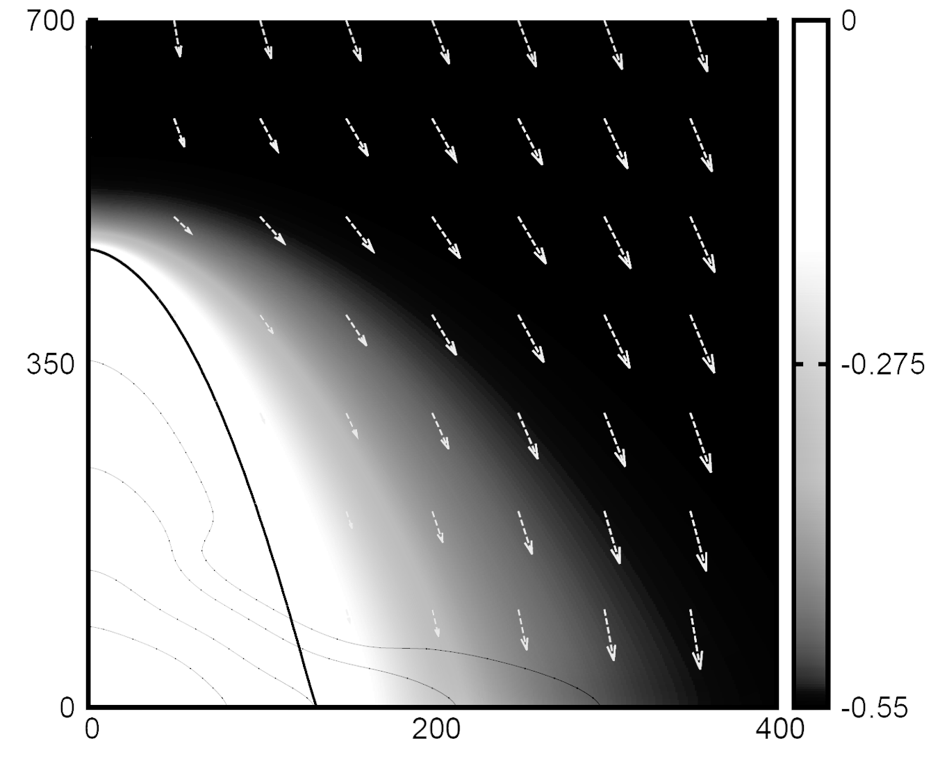
b)

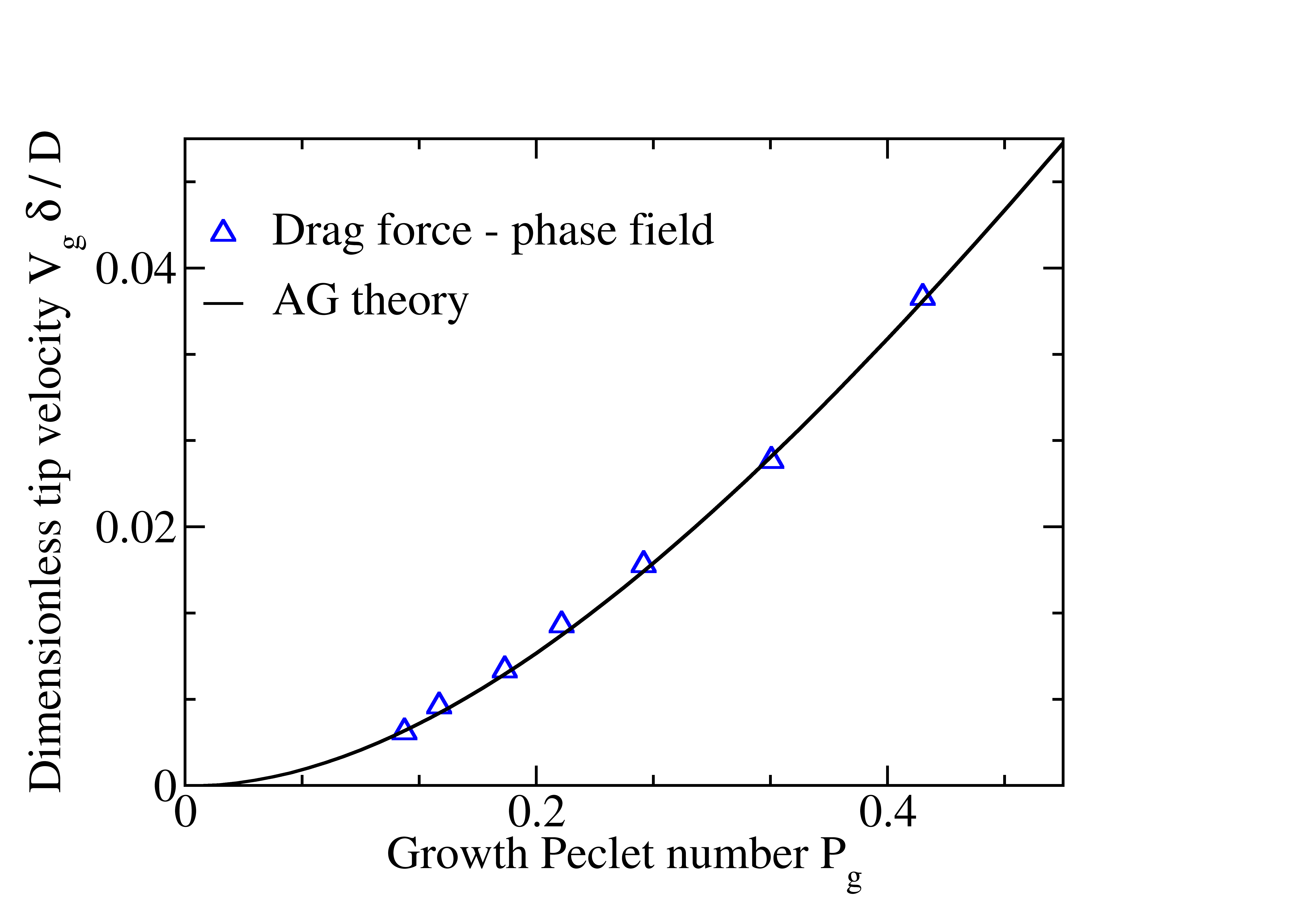
Figure 1: a) A growing dendrite subject to convection. For numerical solution, coupled system of equations Eq. (2), Eq. (3), Eq. (4) and Eq. (9) are solved. The arrow head shows direction while length shows strength of melt flow velocity. b) The dimensionless tip velocity versus the growth Péclet number $P_{\text{g}}$ calculated by the present PF model (triangles) and AG theory Alexandrov and Galenko (2013).

IV Conclusions

A thin-interface analysis of the phase field equations in the presence of melt convection is provided. It is shown that, as in the case of diffusive transport, the thickness of the diffuse interface can be chosen such that its effects on the obtained results are minimized. This prediction is verified by a comparison of the numerical simulation results for dendritic tip velocity and an analytic theory, which accounts for flow effects. As an outlook for further work, it shall be noted that, unlike the temperature or the solute fields, the melt velocity identically vanishes in the solid domain. The non-vanishing normal gradients of the tangential velocity contribute to the shear stress tensor that generates an equal and opposite resulting force on the growing solid. The solid structure, when allowed to move, in turn, influences the melt flow field and thereby transport of heat and solute. In such a case, the unbalanced shear stresses on solid might play an important role.

References

- Boettinger et al. (2002) W. J. Boettinger, J. A. Warren, C. Beckermann, and A. Karma, Annual Review of Materials Research 32, 163 (2002).
- Steinbach (2009) I. Steinbach, Acta Materialia 57, 2640 (2009).
- Caginalp (1989) G. Caginalp, Phys. Rev. A 39, 5887 (1989).
- Karma and Rappel (1996) A. Karma and W.-J. Rappel, Phys. Rev. Lett. 77, 4050 (1996).
- Anderson et al. (2001) D. Anderson, G. McFadden, and A. Wheeler, Physica D: Nonlinear Phenomena 151, 305 (2001).
- Tönhardt and Amberg (1998) R. Tönhardt and G. Amberg, Journal of Crystal Growth 194, 406 (1998).
- Nestler et al. (2000) B. Nestler, A. Wheeler, L. Ratke, and C. Stöcker, Physica D: Nonlinear Phenomena 141, 133 (2000).
- Anderson et al. (2000) D. Anderson, G. McFadden, and A. Wheeler, Physica D: Nonlinear Phenomena 135, 175 (2000).
- Beckermann et al. (1999) C. Beckermann, H.-J. Diepers, I. Steinbach, A. Karma, and X. Tong, Journal of Computational Physics 154, 468 (1999).
- Tong et al. (2001) X. Tong, C. Beckermann, A. Karma, and Q. Li, Phys. Rev. E 63, 061601 (2001).
- Jeong et al. (2001) J.-H. Jeong, N. Goldenfeld, and J. A. Dantzig, Phys. Rev. E 64, 041602 (2001).
- Medvedev and Kassner (2005) D. Medvedev and K. Kassner, Phys. Rev. E 72, 056703 (2005).
- Subhedar et al. (2015) A. Subhedar, I. Steinbach, and F. Varnik, Phys. Rev. E 92, 023303 (2015).
- (14) A. Subhedar, P. Galenko, and F. Varnik, “Thin interface limit of the double sided phase field model with convection,” In preparation.
- Alexandrov and Galenko (2013) D. V. Alexandrov and P. K. Galenko, Phys. Rev. E 87, 062403 (2013).