Protection of Edge transport in Quantum Spin Hall samples:
Spin-Symmetry Based General Approach and Examples

Abstract

Understanding possible mechanisms, which can lead to suppression of helical edge transport in Quantum Spin Hall (QSH) systems, attracted huge attention right after the first experiments revealing the fragility of the ballistic conductance. Despite the very intensive research and the abundance of theoretical models, the fully consistent explanation of the experimental results is still lacking. We systematize various theories of helical transport with the help of the spin conservation analysis which allows one to single out setups with the ballistic conductance being robustly protected regardless of the electron backscattering. First, we briefly review different theories of edge transport in the QSH samples with and without the spin axial symmetry of the electrons including those theoretical predictions which are not consistent with the spin conservation analysis and, thus, call for a deeper study. Next, we illustrate the general approach by a detailed study of representative examples. One of them addresses the helical edge coupled to an array of Heisenberg-interacting magnetic impurities (MIs) and demonstrates that the conductance remains ballistic even if the time-reversal symmetry on the edge is (locally) broken but the total spin is conserved. Another example focuses on the effects of the space-fluctuating spin-orbit interaction on the QSH edge. It reveals weakness of the protection in several cases, including, e.g., the presence of either the U(1)-symmetric, though not fully isotropic, MIs or generic electron-electron interactions.

I Introduction

The theory predicting existence of time-reversal invariant two-dimensional (2D) topological insulators [1, 2, 3], often dubbed Quantum Spin Hall (QSH) samples [4, 5, 6], provoked a huge interest because of its physical beauty and high potential for applications in nanoelectronics, spintronics, and quantum computers. It was realized [7, 8] that the one-dimensional (1D) boundary between trivial and topological insulators, which are distinguished by inversion of the gap in the spectrum of electrons, can host the so-called helical gapless edge modes. Modes of the given helicity possess lock-in relation between their spin and momentum. The Kramers degeneracy guarantees that there are always two counterpropagating modes possessing the same energy and opposite spins. A single-particle scattering, which converts the helical mode into its counterpart from the Kramers doublet, is not allowed without a spin-flip. Thus, at least in the absence of interactions, the helical modes are not liable to backscattering and localization caused by material imperfections. This could provide a possibility to sustain ballistic transport, which possesses the quantized ballistic conductance, $G_{0}=e^{2}/h$ per one QSH edge, in long 1D conductors. The róle of the topologically nontrivial bulk and of time reversal symmetry (TRS) is often reflected in referring to the QSH edge transport as “topologically protected transport” or “transport protected by TRS”.

Transport properties of real samples appeared to be much more complicated than the above described single-particle picture. It became clear already after first measurements that helical QSH transport remains ballistic only in relatively short samples and the conductance may be smaller than $G_{0}$ if the edge length is larger than some critical value [9, 10, 11, 12]. This points out to the presence of not-single-particle backscattering of the helical fermions, which can occur without changing the topological state of the bulk or breaking TRS. The subballistic conductance demonstrates incompleteness of the notion of topologically/TRS protected transport for the interacting helical edges.

The elegancy of the physics of the 2D topological insulators together with promising potential of their application gave a strong push to numerous experimental [13, 14, 15, 16, 17, 18, 19, 20, 21, 22, 23, 24, 25, 26, 27, 28, 29] and theoretical [30, 31, 32, 33, 34, 35, 36, 37, 38, 39, 40, 41, 42, 43] studies, see also references to other papers which are discussed below in more detail. Despite enormous efforts of researchers, the fully consistent theory explaining suppression of QSH helical transport in all experimental setups is still absent and remains the hot topic. On the other hand, an abundance of various theoretical models and some confusions in the terminology addressing the origin of protected transport hamper comprehension of the field.

We would like to somehow brighten such a picture. In this Paper, we discuss helical transport in the QSH samples with- and without the axial spin symmetry of the electrons. We emphasize that, if this symmetry is present, the (sub)ballistic nature of the conductance is fully determined by the (non)conservation of the total spin projection on the axis of the spin symmetry. Importantly, if the total spin projection is conserved, the helical conductance is ballistic regardless of the electron backscattering and of the presence of the TRS on the QSH edge. If, on the contrary, this projection is not conserved, the helical conductance can be suppressed even if the TRS is not broken.

The spin conservation analysis in systems with broken spin axial symmetry is generically more sophisticated. Nevertheless, we will show that such an approach remains a useful tool. In particular, the spin axial symmetry is effectively restored in the experimentally relevant low-temperature limit, and the analysis of the spin conservation allows one to identify the setups where the ballistic conductance can(not) be suppressed.

The paper is organized as follows: the Landauer setup for the helical conductors and basic notations are introduced in Sect.II. Sect.III and IV are devoted to the discussion of the QSH systems with- and without the spin axial symmetry of the electrons, respectively. Sect.III starts with a methodological explanation of the connection between the spin relaxation and the suppression of the helical conductance. Both Sect.III and IV include a brief (though not an exhaustive) review of representative models and theories, which illustrates this connection, and a detailed study of a corresponding example (with- and without the spin axial symmetry), which corroborates the above generic statements and the approach. In the review-like subsections, we critically analyze some contradictive claims on a suppression of the ballistic conductance in the spin preserving setups. This demonstrates that using the spin conservation analysis might help to avoid such inconsistencies.

The example of Sect.III addresses scattering of the helical electrons caused by either uncorrelated or Heisenberg-interacting magnetic impurities (MIs). They are able to cause backscattering of the individual electrons which is accompanied by the spin flip. We argue that such a backscattering has no influence on the linear dc helical conductance if the total spin is conserved. This holds true regardless of a spin ordering which breaks the TRS on the helical edge.

In the example of Sect.IV, we analyze the protection of helical transport against combined effects of the space-fluctuating spin-orbit interaction (SOI) and the scattering of the interacting helical electrons by the MIs. A fully isotopic and short-range correlated array of the MIs is unable to suppress the helical conductance even if the SOI fluctuates. On the other hand, the absence of the spin axial symmetry of the electrons leads to the suppression of the helical conductance by the U(1)-symmetric, though not fully isotropic, MIs. This follows from the spin conservation analysis which is applicable despite the absence of the spin conservation in the laboratory frame.

We conclude the paper by a brief Summary.

II Landauer setup for a helical wire

We focus on the helical modes of the single QSH edge and discuss the linear dc conductance of the system. We conventionally subdivide the edge into three parts: two ideal 1D helical wires connecting leads and a complex scattering region (SR), see Fig.1.

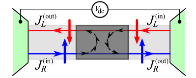
Figure 1: A generic two terminal setup for measuring the helical Landauer conductance: 1D wires (light grey boxes) with two modes of the same helicity (red and blue lines) are connected to 2D leads (colored trapezia). For simplicity, we have illustrated the case where the electron spin quantization axis is well-defined in the wires. The central part – the scattering region – is a conducting region where backscattering (black dashed lines) of the electrons is possible. The dc voltage, $V_{\rm dc}$, is applied to the 2D leads.

Left and right wires are ideal, i.e. contain no sources for the scattering of the helical electrons. The middle part, the SR, is a conducting region where the helical electrons can be scattered. This corresponds to the standard Landauer setup: The SR acts as a composite scatterer while left and right ideal helical wires are identical and play a role of contacts connecting the scatterer and external 2D leads.

II.1 Backscattering inside the SR

The necessary, though not sufficient, condition for suppression of the ballistic conductance is backscattering of the helical electrons inside the SR. Since the single particle backscattering of the helical electrons by a potential disorder is not allowed, it can be caused only by interactions. The nature of these interactions is broad and ranges from various exchange interactions, to electron-electron interactions, to a nontrivial (e.g. fluctuating in space) SOI, to name just a few. Exchange interactions may include those with frozen or dynamical localized spins, the MIs. The latter are often referred to as Kondo impurities even in the weak coupling regime where the Kondo physics is unimportant.

We emphasize that, below, we discuss many examples where backscattering of individual electrons does not suppress the ballistic conductance since transport remains protected. This paradoxical situation is the well-known property of the helical systems. It compels us to distinguish notions of “backscattering” and ”the ballistic transport”, see also the discussion in Sect.III.1.2.

The analysis of the helical conductance in the QSH sample depends on the presence or absence of the electron spin axial symmetry. These two cases are discussed in next Sections.

III QSH systems with
spin axial symmetry of electrons

The focus of this section is on the QSH systems with the spin axial symmetry of the electrons. Namely, we discuss the systems where the spin projection on a given direction is conserved for all non-interacting helical electrons. The Hamiltonian describing free helical 1D Dirac fermions in the left/right wires, Fig.1, reads as:

$$\hat{H}_{0}=-iv_{F}\int{\rm d}x\ \hat{\Psi}^{\dagger}(x)\hat{\sigma}_{z}\partial_{x}\hat{\Psi}(x)\,.$$ (1)

Here $\,v_{F}$ is the Fermi velocity; $\hat{\Psi}=\{\psi_{\uparrow},\psi_{\downarrow}\}^{\rm T}$ is the spinor constructed from the fermionic fields with given spin projections on z-axis; the Pauli matrix $\,\hat{\sigma}_{z}\,$ (and $\,\hat{\sigma}_{x,y}\,$ introduced below) operates in the spinor space. Eq.(1) is the simplest model which describes the edge modes, for example, in those HgTe/CdTe quantum-well heterostructures which possess the axial and inversion symmetry around the growth axis.

The Hamiltonian (1) of the free electrons conserves z-component of their spin which is the starting point for the analysis of the helical conductance. We emphasize that, in the QSH systems with the electron spin axial symmetry, the spin projection unambiguously defines the chirality of right ($R$) and left ($L$) moving electrons with a given helicity. In this case, one can use subscripts $\uparrow,\downarrow$ and $R,L$ on equal footing.

III.1 Spin (im)balance

III.1.1 (Im)balance of currents

The Landauer setup shown in Fig.1 involves incoming, $J_{R,L}^{\rm(in)}$, and outgoing, $J_{R,L}^{\rm(out)}$, chiral charge currents. Assuming reflectionless contacts between the wires and the leads, the incoming currents are fully governed by the leads: $J_{R,L}^{\rm(in)}=ev_{F}\sum_{k}n_{R,L}(k)$, with $e$ and $k$ being the electron charge and momentum. The electronic distribution functions $n_{R,L}$ are determined by the left and right leads, respectively. Outgoing currents are a priori not known.

We consider only those SRs where the charge is conserved and the following charge current balance always holds true:

$$J_{R}^{\rm(in)}+J_{L}^{\rm(in)}=J_{R}^{\rm(out)}+J_{L}^{\rm(out)}.$$ (2)

Similar to the charge currents, we introduce incoming, $S_{R/L}^{\rm(in)}$, and outgoing, $S_{R/L}^{\rm(out)}$, currents of the electron spin projected on the quantization axis. The interaction induced backscattering can (or cannot) violate the spin conservation in the SR. Therefore, we cannot presume a robust balance of the spin currents. Possible violation of the spin conservation can be characterized by the spin imbalance: $\delta S=(S_{R}^{\rm(in)}+S_{L}^{\rm(in)})-(S_{R}^{\rm(out)}+S_{L}^{\rm(out)})$. Using the well-known relation between the charge and spin currents in the QSH systems with the axial symmetry and the certain helicity on the edges, $S_{R}^{\rm(in/out)}=J_{R}^{\rm(in/out)}/2e$, and $S_{L}^{\rm(in/out)}=-J_{L}^{\rm(in/out)}/2e$, we express $\delta S$ via $J_{R/L}^{\rm(in/out)}$:

$$\delta S=\left(J_{R}^{\rm(in)}-J_{L}^{\rm(in)}-J_{R}^{\rm(out)}+J_{L}^{\rm(out)}\right)/2e.$$ (3)

It follows form Eq.(3) that, if the SR is spin conserving, the helical conductance remains ballistic. Namely, if $\delta S=0$, then [recalling Eq.(2)] we obtain:

$$J_{\mu}^{\rm(in)}=J_{\mu}^{\rm(out)},\ \mu=R,L.$$ (4)

Therefore, the total electric current through the system, $J_{\rm tot}=J_{R}^{\rm(in)}-J_{L}^{\rm(out)}=J_{R}^{\rm(out)}-J_{L}^{\rm(in)}$, can be expressed via incoming currents:

$$J_{\rm tot}=J_{R}^{\rm(in)}-J_{L}^{\rm(in)},$$ (5)

which are fully determined by the external voltage $V_{\rm dc}$ and by contacts between the external leads and the clean helical wires. Thus, if $\delta S=0$, the Landauer conductance, $G_{\rm dc}=J_{\rm tot}/V_{\rm dc}$, is not sensitive to the presence of the SR in the circuit. In the case of the reflectionless contacts [44], one arrives at $G_{\rm dc}=G_{0}$ regardless of internal details of the spin (and charge) conserving SR, including the interaction induced backscattering inside the SR.

If the SR is not spin-conserving and there is the spin imbalance, $\delta S\neq 0$, the backscattering in the SR results in the so-called backscatering current, $J^{\rm(BS)}_{R,L}=J_{R,L}^{\rm(out)}-J_{R,L}^{\rm(in)}$, which suppresses the ballistic helical conductance.

III.1.2 Ballistic transport vs. backscattering

We come across an unusual situation where the helical Landauer conductance is ballistic despite the interaction induced backscattering inside the spin preserving SR. Therefore, we should distinguish concepts of ballistic transport and backscattering and refer to the regime $G_{\rm dc}=G_{0}$ as “ballistic”, though the helical electrons can be backscattered. This remarkable robustness of the ballistic conductance with respect to backscattering is the direct consequence of helicity and makes the physics of the helical 1D wires distinct from that of usual (non-helical) 1D conductors [45] where any backscattering efficiently suppresses dc transport.

III.1.3 Conditions for the spin conservation

The explicit calculation of the currents is often a very complex task. A feasible and physically transparent alternative is provided by the analysis of the spin conservation in the SR.

An obvious sufficient condition for the spin conservation is the global spin U(1) symmetry, $\exp(i\hat{S}_{z}\alpha)\hat{H}_{\rm tot}\exp(-i\hat{S}^{\rm tot}_{z}\alpha)=\hat{H}_{\rm tot}$, with $\hat{S}^{\rm tot}_{z}$ and $\hat{H}_{\rm tot}$ being the total (of the SR and of the wires) spin operator and Hamiltonian respectively. This requirement is sufficient but, generally speaking, not necessary, cf. Sect.IV.3.

Several specific examples of spin preserving and non-preserving setups are given in the next Subsection. Below, we use terms “the spin U(1) symmetry” and the above discussed “spin conservation” on equal footing.

III.2 Spin (non)preserving setups
and helical transport

Interaction with a single magnetic impurity and nanomagnets: An exchange interaction of the helical electrons with the MI can result in backscattering accompanied by the spin-flip. That is why the MIs were considered as a serious obstacle for ballistic helical transport. The study of the Kondo physics for the XXZ-anisotropic MI immersed in the helical Luttinger liquid erroneously predicted suppression of the helical conductance at finite temperatures [46]. In reality, such an impurity backscatters the helical electrons but does not break the spin U(1) symmetry and, therefore, cannot influence the dc conductance [47]. XYZ-anisotropic MIs violate the spin conservation and are able to suppress the ballistic conductance but only if they are not Kondo screened. This requires either the temperature being larger than the Kondo temperature, $T>T_{K}$, or a large value of the Kondo spin, $S>1/2$ [48, 49]. The Kondo screening of the XYZ-anisotropic spin-1/2 MI restores the spin conservation at $T\to 0$ and, thus, neutralizes the destructive effect of such an impurity on the ballistic conductance [50]: $G_{\rm dc}$ becomes equal to $G_{0}$ at $T\ll T_{K}$.

Coupling of the MI to additional degrees of freedom can result in a finite spin relaxation rate of the MI. It violates the applicability of the spin conservation analysis and might lead to the subballistic conductance. Some examples of this effect have been reported in Refs.[36, 40]: the hyperfine interaction couples the helical electrons to the nuclei spins located near the edge. The latter are, in turn, coupled to the spins in the bulk. This provides a “leakage” of the spins to the bulk and suppresses the helical conductance at very low temperatures [36]. Related effects are substantially material-dependent and are often very weak. For instance, in such an archetypal material as HgTe/(Hg,Cd)Te, they are expected to be pronounced only in long samples, $L\gtrsim 4\mbox{mm}$, at ultralow temperatures, $T\lesssim 5\mbox{mK}$ [40]. Since we address more universal mechanisms, we follow the majority of studies in the field and do not take into account additional (beyond those caused by the electron-spin exchange coupling) spin relaxations in the present paper.

The consideration of the MI, which backscatters the helical electrons in the SR, can be easily extended to macroscopic magnetic scatterers consisting of a finite ensemble of dynamically interacting spins. For example, instead of the single MI, one can consider a macroscopic nanomagnet which can be phenomenologically described by a time-dependent vector of magnetisation [51]. If there is no spin relaxation inside the magnet, the conductance reaches $G_{0}$ after some transient governed by accumulation of an excessive spin, which flows into the magnet from the biased helical wires.

An attempt to develop a microscopic theory of the nanomagnet attached to the helical edge has been presented in Ref.[52]. The authors of this paper have used the Kane-Mele-Hubbard model, where the nanomagnet is expected to appear spontaneously at small temperatures near a dislocation placed close by the helical edge. The microscopic origin of this effect is the electron interaction. By employing a self-consistent mean-field approximation (MFA), one can come to a doubtful conclusion on a suppression of the helical conductance by such a nanomaget even at $T\to 0$ [52]. Indeed, since the magnetization is frozen (the basic assumption of the MFA) it certainly violates the spin conservation and can suppress the helical conductance. However, the Hamiltonian of the Kane-Mele-Hubbard model has the global spin U(1) symmetry and, therefore, the spin conservation analysis puts the MFA prediction in question. We believe that fluctuations are crucially important since they bring to life dynamics of the effective nanomagnet which could restore the ballistic value of the conductance. Thus, this interesting model deserves a further study.

A detailed and more rigorous microscopic study of the influence of the MI array (correlated or uncorrelated) on the helical conductance is presented in the next Subsection. We will show that our microscopically obtained results are in perfect agreement with the spin conservation analysis.

Interaction between electrons and two-particle backscattering: Various electron interactions can yield two-particle backscattering which is able to suppress the ballistic conductance if the spin conservation is violated. For example, anisotropic electron spin interactions on a lattice can govern the umklapp two-electron backscattering which suppresses helical transport [8]. The electron-electron interaction in quantum dots (charge puddles) attached to the helical edge was considered in Refs.[53, 54]. The spin non-conserving interaction of the electrons inside the dots provides the spin relaxation and makes the helical edge conductance subballistic.

Contacts between the helical wires and the SR: One should keep in mind that the contacts between the helical wires and the SR themselves can violate conservation laws and suppress ballistic transport. For instance, one could erroneously surmise that the SR containing usual (non-helical) 1D spinful modes and a spinless disorder does not violate the spin conservation but, nevertheless, suppresses the conductance via the mechanism of Anderson localization. As a matter of fact, there is no contradiction since any connection of helical- and non-helical wires in a series violates validity of the conservation laws. Namely: (i) The contact, where the spin is preserved, would violate unitarity of the S-matrix (i.e., would violate the charge conservation) describing such a connection. This directly follows from a different number of channels with a given spin in the non-helical- and helical wire, e.g., $R_{\uparrow}$ and $L_{\uparrow}$ in the non-helical wire and only $R_{\uparrow}$ in the helical one. (ii) The only other possibility for the connection in series is to allow the helical electron to change its spin inside the contact. Clearly, this possibility is incompatible with the total spin conservation.

III.3 Helical modes interacting with a Kondo-Heisenberg array - a case study

Let us now elaborate at the microscopic level how the above explained spin conservation analysis works in the case of the helical edge coupled to an array of the MIs. Such systems regain at present an increased attention since they can provide a platform for the realization of chiral Majorana fermions [55]. The MI can be correlated either via the indirect exchange interaction supported by the itinerant electrons [usually referred to as ”the Kondo array” (KA)] or via the both indirect and direct Heisenberg interaction [usually named ”the Kondo-Heisenberg array” (KHA)].

The influence of the dense KA on the conductivity of the helical edge was studied in Refs.[56, 57]. The high density of the MIs means that the Kondo effect is overwhelmed by the MI correlations [58] and the MIs remain unscreened at low temperatures. It was shown that if the helical electrons are scattered by the KA with the random XYZ-anisotropy one comes across Anderson localization of the charge carriers [56] while, in the spin U(1)-symmetric setup, the backscattering leads only to the renormalization of the Drude peak in the dc conductivity. Based on a straightforward though a kind of superficial analogy with the physics of usual (not helical) interacting 1D wires [59, 60, 61], a ballistic nature of the dc conductance in the spin preserving setup was conjectured in Ref.[56]. We now demonstrate that this conjecture is correct and extend the theory to the dense KHA where the Heisenberg interaction of the MIs may govern the TRS-breaking spin ordering.

The total Hamiltonian describing the helical edge modes, which interact with the KHA (see Fig.2), is $\hat{H}_{\rm full}=\hat{H}_{0}+\hat{H}_{H}+\hat{H}_{b}+\hat{H}_{V}$. It includes the fermionic and MI parts, $\hat{H}_{0}$ and $\hat{H}_{H}$, respectively, and the voltage source part $\hat{H}_{V}$ which depends only on the fermionic operators. $\hat{H}_{b}$ is the Hamiltonian of the fermion-MI interaction which describes backscattering induced by MIs. In the spin-conserved setup, it reads as follows:

$$\hat{H}_{b}=\sum_{j}\!\!\hat{S}^{+}_{j}[J_{K}\psi^{\dagger}_{\downarrow}\psi_{\uparrow}](x_{j})+h.c.$$ (6)

Here the sum runs over MI positions $x_{j}$, $\,J_{K}\,$ is the position dependent coupling constant between the MIs and the fermions; $\,\hat{S}^{\pm}_{j}=e^{\pm 2ik_{F}x_{j}}(\hat{S}_{x}\pm i\hat{S}_{y})_{j}\,$ are rotated raising/lowering operators of the MIs. Eq.(6) corresponds to the U(1)-symmetric XXZ-coupling with $J_{K}=J_{K}^{(x)}=J_{K}^{(y)}$. To simplify discussion of this example, we take into account neither electron-electron interactions nor forward-scattering generated by the component $J_{K}^{(z)}$ though including them is straightforward and does not change our conclusions.

The spin Hamiltonian $\hat{H}_{H}$ describes the direct Heisenberg exchange interaction (of quantum Ising type) between the z-components of the MI spins:

$$\hat{H}_{H}=\sum_{j}J_{H}(x_{j})\hat{S}_{z}(j)\hat{S}_{z}(j+1)\,;$$ (7)

where $J_{H}$ is the position dependent coupling constant. For concreteness, we have chosen the exchange interaction between nearest neighbors. The inter-impurity distance $\xi_{s}(j)=x_{j+1}-x_{j}$ can fluctuate in space if the spin array is geometrically disordered.

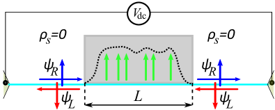
Figure 2: (color on-line) 1D wire with helical electrons, $\psi_{R/L}$ or equivalently $\psi_{\uparrow/\downarrow}$, coupled to the Kondo-Heisenberg array (green arrows) located inside the SR (shadowed rectangle). Density of the MIs (dotted line) vanishes outside the SR and fluctuates in space inside it. The interaction constants, $J_{K,H}$ can also depend on the coordinate.

The MI density is $\rho^{(d)}_{s}(x)=\sum_{j}\delta(x-x_{j})$ for the discrete array. Its smeared counterpart, $\rho_{s}(x)$, vanishes outside the SR and is finite and coordinate-dependent inside it.

Our starting point is similar to that of Refs.[59, 62]: We express the electric current via a convolution of the non-local conductivity, $\sigma(x,x^{\prime};\omega)$, and an inhomogeneous electric field $\,E(\omega,x^{\prime})$:

$$j(x,t)=\int{\rm d}x^{\prime}\int\frac{{\rm d}\omega}{2\pi}e^{-i\omega t}\sigma(x,x^{\prime};\omega)E(\omega,x^{\prime})\,.$$ (8)

$E(\omega,x)$ is governed by the applied voltage. Next, we bosonize the theory, use the technique of the functional integrals on the imaginary time, and describe the fermions by the standard Lagrangian of the helical Luttinger Liquid with the source term [45, 8]:

$${\cal L}_{\rm HLL}=\left[(\partial_{\tau}\phi)^{2}+(v_{F}\partial_{x}\phi)^{2}\right]/2\pi v_{F}+i\chi\phi\,.$$ (9)

The Fourier transform of the bosonic Green’s function (GF), $G(x,x^{\prime};\tau)=-\langle\phi(x^{\prime},\tau)\phi(x,0)\rangle$, yields the Matsubara conductivity: $\sigma(x,x^{\prime};\bar{\omega})=(e^{2}\bar{\omega}/\pi^{2})\,G(x,x^{\prime};\bar{\omega})\,.$ The Lagrangian describing the spin-conserving backscattering reads:

$${\cal L}_{b}[n_{z},\alpha,\phi]=2s\rho_{s}(x)J_{K}(x)\sqrt{1-n^{2}_{z}}\cos(\alpha-2\phi)\,.$$ (10)

Here we parameterize each localized spin by its azimuthal angle, $\,\alpha$, and projection on $z$-axis, $\,|n_{z}|\leq 1$: $S^{\pm}=se^{\pm i\alpha}\sqrt{1-n^{2}_{z}}\,,\ S_{z}=sn_{z};$ with $s$ being the spin value. This parametrization requires the Wess-Zumino term in the Lagrangian [63, 64]:

$${\cal L}_{\rm WZ}[n_{z},\alpha]=is\rho_{s}(1-n_{z})\partial_{\tau}\alpha\,.$$ (11)

Let us now shift the spin phase $\tilde{\alpha}=\alpha-2\phi$. The full Lagrangian in the new variables is

$${\cal L}={\cal L}_{\rm HLL}[\phi,\chi]+{\cal L}_{\rm WZ}[n_{z},2\phi]+{\cal L}_{\rm MI}[n_{z},\tilde{\alpha}]\,.$$ (12)

Here ${\cal L}_{\rm MI}\equiv{\cal L}_{b}[n_{z},\tilde{\alpha},0]+{\cal L}_{H}[n_{z}]+{\cal L}_{\rm WZ}[n_{z},\tilde{\alpha}]$ is the MI Lagrangian; ${\cal L}_{H}$ describes the Heisenberg interaction of the MIs.

The coupling between the fermionic and MI sectors is reflected in Eq.(12) only by ${\cal L}_{\rm WZ}[n_{z},2\phi]$. Its contribution vanishes in the dc limit and the MI variables drop out from the equation for the dc conductivity which reduces to that of the clean helical wire, see the proof in Appendix A. Therefore, coupling between the helical modes and the spin-preserving KHA is unable to change the ballistic dc helical conductance as one expects from the above explained generic arguments.

Dense and large KHAs can host various spin orders [65]. If $J_{H}$ exceeds a critical value, $J_{H}^{*}$, the crossover (the quantum phase transition in the infinite system) of the Ising type occurs at zero temperature and the component $S_{z}$ on the edge of the QSH sample acquires a non-zero semiclassical average value, $s\langle n_{z}\rangle$ [66]. This means that the TRS can be spontaneously broken on the QSH edge . Nevertheless, the helical dc transport remains ballistic and protected as soon as the total spin is conserved. These arguments show the secondary importance of the TRS on the edge for the protection of the helical transport. Note that the fermion backscattering by the magnetically ordered KHA requires an energy of the order of the domain wall energy, ${\cal E}_{\rm DW}$ . Therefore, it is expected to be suppressed in regimes where all characteristic energy scales are $\ll{\cal E}_{\rm DW}$.

We emphasize that the dc helical transport in the current example is sensitive neither to the profile of the spin density, $\rho_{s}(x)$, nor to the spatial inhomogeneity of the coupling constants, $J_{K,H}(x)$. This is the exclusive property of the helical system. On the other hand, the ac conductance might be sensitive to details of the setup.

Let us conclude this Section with an example which demonstrates a predictive power and usefulness of the spin conservation analysis. So far, we have taken into account only the Heisenberg interaction between z-components of the MI spins. The presence of the spin-preserving in-plane Heisenberg interaction of the MIs, ${\cal L}_{H}^{\rm(xy)}\propto\rho_{s}e^{-2ik_{F}\xi_{s}}S^{+}(x+\xi_{s})S^{-}(x)+h.c.$, makes the analysis of the dc conductance technically very complicated. In particular, the phase $\phi$ cannot be gauged out simultaneously from the Lagrangians ${\cal L}_{b}$ and ${\cal L}_{H}^{\rm(xy)}$. Qualitative arguments confirming the helical ballistic conductivity are given in Ref.[66] for the case of an infinite system where the total spin is conserved. However, based on the spin conservation analysis, one can state without explicit calculations that the conductance remains ballistic in this complicated setups because the total spin is conserved.

IV QSH systems with broken
spin axial symmetry of electrons

Another class of the QSH systems embraces those TRS-invariant 2D topological insulators where the spin axial symmetry of the electrons is broken. As a result, the electron spin quantization axis cannot be uniquely defined for all helical electrons and the z-component of the electron spin is no longer conserved. Well-known microscopic mechanisms, which are compatible with the TRS and break the spin axial symmetry, are the bulk- and the structural inversion asymmetry [69, 70]. The effects of the broken axial symmetry can be described by an effective spatially homogeneous Rashba SOI in the 2D bulk. Close to the 1D edge of the QSH sample, the Rashba SOI can be inhomogeneous and strongly fluctuate.

The absence of the spin axial symmetry makes the applicability of the above explained spin conservation analysis more sophisticated. A few particular cases are discussed below.

IV.1 Spin texturing in momentum space

If the TRS-invariant QSH system possesses the homogeneous Rashba SOI in the bulk, the spins of the edge electron remain antiparallel only for two states of the Kramers doublet of the same energy (i.e. for two modes with momentums $\pm k$) while the direction of the spin quantization depends on the electron energy (i.e. on $|k|$), the so-called spin-texturing (ST) [71]. In that case and unlike the Hamiltonian Eq.(1), one should distinguish the chiral and spin bases of the fermions. These bases are related by the unitary transformation which respects TRS: $\tilde{\Psi}=\{\psi_{R},\psi_{L}\}^{\rm T}=\hat{B}^{\dagger}_{k}\hat{\Psi},\ \hat{B}^{\dagger}_{k}\hat{B}_{k}~{}=~{}1,\ \hat{B}_{k}=\hat{B}_{-k}$. The chiral basis is needed to calculate the charge current carried by the helical electrons. The Hamiltonian, which accounts for the ST in the momentum space, reads as:

$$H^{(k)}_{\rm ST}=v_{F}\sum_{k}k\,\hat{\Psi}^{\dagger}(k)\hat{B}_{k}\hat{\sigma}_{z}\hat{B}^{\dagger}_{k}\hat{\Psi}(k).$$ (13)

As opposed to $\hat{H}_{0}$, the Hamiltonian $H^{(k)}_{\rm ST}$ does not conserve z-component of the electron spin. Therefore, in a general case, one cannot use the spin conservation analysis to check the ballistic nature of the conductance. The obvious exception is the case of zero temperature where transport is carried by the electrons at $k_{F}$ and the product $\hat{B}_{k_{F}}\hat{\sigma}_{z}\hat{B}^{\dagger}_{k_{F}}$ determines the direction of the spin quantization axis for the conduction electrons. Hence, the ST becomes irrelevant at $T=0$ because of the absence of the allowed phase space for the electrons and the nature of the helical conductance (ballistic or subballistic) is fully determined by the properties of the SR similar to the above discussed cases with the spin axial symmetry.

If temperature is finite, the ST violates the electron spin conservation and the helical conductance can become subballistic. The well-known effect of the ST is the suppression of the helical conductance caused by the inelastic (accompanied by the energy transfer) backscattering of the (disordered) helical electrons which either interact with each other [72, 73, 74] or experience an influence of a noise [75]. Less expected effect is an influence of the unscreened isotropic MI on helical transport of the noninteracting electrons, see Ref.[76] where the example of the spin-1/2 MI has been studied at $T>T_{K}$. The underlying mechanism is the successive backscattering of the helical electrons which have the same chirality but different energies. We remind the readers that, if there is no ST, the unscreened isotropic or even U(1) symmetric spin-1/2 MI can backscatter one after another only electrons of different chirality, thus, the dc conductance remains unaffected [47].

IV.2 Spin texturing in real space

The spin texturing in real space originates in models where the direction of the spin quantization on the helical edge is space-dependent. This could result from the inhomogeneously changed direction of the SOI governed by a combined effect of the spin-diagonal (Dresselhaus) and the spin-off-diagonal (Rashba) SOIs [70, 77]. The latter does not violate the topologically non-trivial state of the QSH sample but can be strong on its edges. To describe the QSH edge with the spatially fluctuating SOI, one needs an extended version of the Hamiltonian $\hat{H}_{0}$, Eq.(1), which reads as follows:

$$\hat{H}^{(x)}_{\rm ST} = -i\frac{v_{F}}{2}\int{\rm d}x\ \hat{\Psi}^{\dagger}(x)\left\{\left({\bm{n}}(x)\cdot{\bm{\sigma}}\right),\partial_{x}\right\}_{+}\hat{\Psi}(x)=$$ (14)

$$= -iv_{F}\int{\rm d}x\ \hat{\Psi}^{\dagger}(x)\left({\bm{n}}(x)\cdot{\bm{\sigma}}\right)\partial_{x}\hat{\Psi}(x)-$$

$$-i\frac{v_{F}}{2}\int{\rm d}x\ \hat{\Psi}^{\dagger}(x)\left(\bigl{[}\partial_{x}{\bm{n}}(x)\bigr{]}\cdot{\bm{\sigma}}\right)\hat{\Psi}(x)\,;$$

see Refs.[78, 79, 77, 80]. In Eq.(14), ${\bm{\sigma}}=\{\hat{\sigma}_{x},\hat{\sigma}_{y},\hat{\sigma}_{z}\}$ and the anticommutator $\{\ldots\}_{+}$ ensures the Hermiticity of $\hat{H}^{(x)}_{\rm ST}$. In the Landauer setup of Fig.1, the vector ${\bm{n}}$ depends on the coordinate inside the SR and is fixed by the equality ${\bm{n}}=\{0,0,1\}$ at contacts between the SR and the helical wires and in both wires. Clearly, the Hamiltonian Eq.(14) coincides with $\hat{H}_{0}$, Eq.(1), if ${\bm{n}}=\{0,0,1\}={\rm const}$ in the entire sample. We emphasize that Eq.(13) and Eq.(14) describe two principally different physical mechanisms of the ST and there is no simple relation between these equations. Using Eq.(14) in the QSH systems with the broken axial symmetry implies that the product $\hat{B}_{k_{F}}\hat{\sigma}_{z}\hat{B}^{\dagger}_{k_{F}}$ yields the mean direction of the electron spin quantization axis and the SOI fluctuations overwhelm the temperature-dependent effects of the ST at low temperatures, $T/{\cal E}_{st}\ll 1$ (${\cal E}_{st}$ is the energy scale of the ST).

The electron spin density does not commute with Hamiltonian (14). Hence, the total spin is not conserved in the laboratory frame and one could presume that transport could be sub-ballistic even on clean (without magnetic scatterers) edges with space-fluctuating SOI [77]. This guess is incorrect. The role of the spin conservation, which is a kind of masked in the model (14), for the protection of transport was noticed in Ref.[80]. We will explicitly demonstrate this in the next Section by using a simple and straightforward rotation of the fermionic basis. We will use the spin conservation analysis in the rotated frame to make conclusive predictions on the combined effects of the fluctuating SOI, the KHA and the electron-electron interactions.

IV.3 Combined influence of fluctuating SOI, KHA,
and electron interaction on helical conductance
- a case study

Let us now explain how to uncover the spin conservation in the QSH edges with the space-fluctuating (but static) direction of the spin quantization in the most straightforward way. First, we explain the method by using the example of the clean Hamiltonian (14) and further use the spin conservation analysis to study combined effects of the fluctuating SOI and the scattering by the KHA in the presence of the electron-electron interaction.

The full Hamiltonian consists of five parts: $\hat{H}_{\rm full}=\hat{H}^{(x)}_{\rm ST}+\hat{H}_{\rm e-KA}+\hat{{\cal H}}_{H}+\hat{H}_{\rm e-e}+\hat{H}_{V}$, where $\hat{H}_{\rm e-KA}$ and $\hat{H}_{\rm e-e}$ describe the exchange interaction of the helical electrons with the KA and the electron-electron interaction, respectively, and are specified below in Eqs.(18,22). $\hat{{\cal H}}_{H}$ is the Hamiltonian of the Heisenberg interaction between the MIs. In the case of the ZZ-interaction, $\hat{{\cal H}}_{H}$ reduces to Eq.(7). In this section, we will explicitly take into account the in-plane Heisenberg interaction, see Eq.(20) below.

For simplicity, we fix the strength of the SOI, such that $|{\bm{n}}(x)|=1$, and parameterize the coordinate-dependent direction of the SOI inside the SC by polar, $\theta$, and azimuthal, $\varphi$, angles: ${\bm{n}}=\{\cos(\varphi)\sin(\theta),\sin(\varphi)\sin(\theta),\cos(\theta)\}$. The boundary condition ${\bm{n}}=\{0,0,1\}$ implies that $\theta=0$ at junctions of the SR with the connecting helical wires. We further assume that the coordinate dependence of ${\bm{n}}$ inside the SC is slow on the scale of the lattice spacing.

Let us, at first, diagonalize the Hamiltonian (14) by using the unitary transformation of the fermionic basis $\tilde{\Psi}=\hat{g}^{\dagger}\hat{\Psi}$ with the matrix $\hat{g}\in\rm{SU(2)}$ being parameterized by the angles $\{\phi,\theta\}$:

$$\hat{g}=e^{-i\frac{\varphi}{2}\hat{\sigma}_{3}}e^{-i\frac{\theta}{2}\hat{\sigma}_{2}},\quad\hat{g}^{\dagger}\left({\bm{n}}\cdot{\bm{\sigma}}\right)\hat{g}=\hat{\sigma}_{3}.$$ (16)

$\hat{g}=1$ outside the SR because of the boundary conditions for ${\bm{n}}$. Changing to the $\tilde{\Psi}$-basis, we find

$$\hat{H}^{(x)}_{\rm ST}=-v_{F}\int{\rm d}x\tilde{\Psi}^{\dagger}\left\{i\hat{\sigma}_{3}\partial_{x}+\frac{1}{2}\cos(\theta)[\partial_{x}\varphi]\right\}\tilde{\Psi}\,;$$ (17)

see algebraic details in Appendix B.

The new frame, where the Hamiltonian (17) is defined, rotates inside the SR together with the SOI. $S_{z}$ spin component of the fermions is manifestly conserved in this rotating frame. One can give the following interpretation to that result: The electron with a given z-component of the spin enters the SR where the electron spin follows the SOI direction. The initial direction of the electron spin is restored after the electron leaves the SR and, thus, the spin conservation law holds true because of the boundary conditions at the contacts of the SR with the left/right helical wires. The spin conservation in the rotating frame suggests that the helical conductance can remain ballistic in spite of the absence of the global spin quantization axis in the laboratory frame. Indeed, both terms in Eq.(17) are diagonal, the term containing $\cos(\theta)$ is an effective forward-scattering potential; hence, there is no backscattering in Eq.(17) and the Landauer conductance must be ballistic, as expected [80].

The protection of the helical conductance against the influence of the fluctuating SOI on the clean and non-interacting edge is in general subtle and can be destroyed, e.g., by non-locality of the SOI fluctuations or by a curvature in the dispersion relation of the helical electrons [81]. On a formal level, these phenomena break the spin conservation in the rotating frame. Besides, the simple form of the diagonalized Hamiltonian (17) can be obtained only for the stationary SOI fluctuations. If these fluctuations are dynamical, the rotation by the matrix $\hat{g}$ does not yield a conclusive information and does not help to prove the ballistic nature of the helical conductance. For instance, the model similar to Eq.(14) can appear due to the deformation of the QSH edge by acoustic phonons [82]. In this case, the deviation of the spin-quantization axis from z-direction is a dynamical degree of freedom, which can be expressed via phonon operators. The theory of the electron-phonon coupling becomes effectively non-local and the helical conductance becomes sub-ballistic at finite temperatures due to the inelastic backscattering of the electrons by phonons [82].

If the SOI fluctuations are static, the above described simple though helpful method allows us to consider the SRs with- and without the fermion scattering on equal footing. Let us gradually make the problem more complicated and, at the next step, include into consideration the scattering caused by the KA. The spin U(1)-invariant Hamiltonian of the exchange interaction between the itinerant electrons and the MIs reads:

$$\hat{H}_{\rm e-KA} = \sum_{j}\hat{\Psi}^{\dagger}(x_{j})({\bm{S}}(j)\hat{J}\cdot{\bm{\sigma}})\hat{\Psi}(x_{j}),$$ (18)

$${\bm{S}}(j) = \{\tilde{S}_{x}(j),\tilde{S}_{y}(j),\hat{S}_{z}(j)\}\,.$$

We have introduced a diagonal matrix of the Kondo coupling constants $\hat{J}\equiv{\rm diag}(J_{K},J_{K},J_{K}^{(z)})$. X- and Y-spin components are related to the above introduced rotated spin operator $\tilde{S}_{x}=(\hat{S}^{+}+\hat{S}^{-})/2$, $\tilde{S}_{y}=-i(\hat{S}^{+}-\hat{S}^{-})/2$. Combined effects of the randomly fluctuating SOI and a single MI has been considered in Ref.[83]. The authors of this paper have focused on the interplay of the Rashba disorder and and off-diagonal anisotropy reflected by off-diagonal entries of the matrix $\hat{J}$. We will show below that even a simpler anisotropy of the XXZ-type (the diagonal matrix $\hat{J}$ and the U(1)-symmetric coupling in the laboratory frame) suffices to suppress the helical conductance if the SOI fluctuates.

We re-write $\hat{H}_{\rm e-KA}$ in the rotated fermionic basis and simultaneously do an arbitrary unitary transformation of the MI spin operators, ${\bm{S}}\rightarrow{\cal S}$. $\hat{H}_{\rm e-KA}$ in the rotated bases reads as:

$$\hat{H}_{\rm e-KA}=\sum_{j}\tilde{\Psi}^{\dagger}(x_{j})({\cal S}(j)\tilde{J}\cdot{\bm{\sigma}})\tilde{\Psi}(x_{j}),\ \tilde{J}\equiv\hat{R}^{T}_{\cal S}\hat{J}\hat{R}_{\Psi}.$$ (19)

The orthogonal matrices $\hat{R}_{{\cal S},\Psi}\in\mbox{SO(3)}$ result from the unitary rotation of the spins and the fermions, respectively. $\hat{R}_{\Psi}$ is parameterized by the angles $\{\phi,\theta\}$ and $\hat{R}_{{\cal S}}$ – by another independent set of the Euler angles, see Appendix C. Clearly, the z-component of the total (of the helical electrons and of the MIs) spin is conserved in the rotated bases if (i) $\tilde{J}_{kl}=0$ for the entries $\{k,l\}=\{1,3\},\{2,3\},\{3,1\},\{3,2\}$; (ii) $\tilde{J}_{11}=\tilde{J}_{22}$; and (iii) $\tilde{J}_{12}=-\tilde{J}_{21}$. This is possible IFF $J_{K}=J_{K}^{(z)}$, i.e. IFF the bare exchange interaction is isotropic. After choosing $\hat{R}_{\cal S}=\hat{R}_{\Psi}$, we reduce Eq.(19) to the isotropic version of the exchange interaction considered in Sect.III.3 at $J_{H}=0$. Based on the above discussion, we conclude that the conductance remains ballistic in the system where the direction of the SOI rotates in the SR even if the SR contains the MIs isotropically coupled (in the laboratory and rotating frames) to the conduction electrons. Any anisotropy of the exchange coupling between the helical electrons and MIs results in the violation of the spin conservation in the rotating frame and, thus, removes the protection of the helical conductance. For example, if the rotated coupling matrix has two coinciding finite diagonal elements $\tilde{J}_{11}=\tilde{J}_{22}\neq 0$ but one non-zero off-diagonal element $\tilde{J}_{13}\neq 0$, the subballistic correction to the helical conductance in the absence of the Kondo screening is $\delta G_{\rm aniso}/G_{0}\propto\tilde{J}_{11}^{2}\tilde{J}_{13}^{2}/(\tilde{J}_{11}^{2}+\tilde{J}_{33}^{2}/2+\tilde{J}_{13}^{2})$, see the derivation and discussion in Ref.[48].

The above consideration can be straightforwardly extended to the scattering of the helical electron by the KHA. We start from the spin-preserving Heisenberg interaction in the laboratory frame:

$$\hat{{\cal H}}_{H} = \sum_{j}\left({\bm{S}}(j)\hat{J}_{H}(j)\cdot{\bm{S}}(j+1)\right)\,,$$ (20)

$$\hat{J}_{H}(j) = {\rm diag}(J_{H}^{\perp},J_{H}^{\perp},J_{H})_{x=x_{j}}\,.$$

We rotate the spin degrees of freedom

$$\hat{{\cal H}}_{H}=\sum_{j}\left({\cal S}(j)\hat{R}^{T}_{S}(j)\hat{J}_{H}(j)\hat{R}_{S}(j+1)\cdot{\cal S}(j+1)\right)\,.$$ (21)

If SOI variations are so smooth that the difference between the SOI at the space points $x_{j}$ and $x_{j+1}$ can be neglected, we obtain $\hat{R}^{T}_{S}(j)\hat{J}_{H}(j)\hat{R}_{S}(j+1)\simeq\hat{R}^{T}_{S}(j)\hat{J}_{H}(j)\hat{R}_{S}(j)$ which reduces to the spin preserving form IFF $J_{H}^{\perp}(x_{j})=J_{H}(x_{j})$, cf. analysis of Eq.(19). Thus, the total spin is conserved in the rotating frame and, based on the results of Sect.III.3, we conclude that the ballistic helical conductance remains protected if both the Kondo- and Heisenberg couplings are isotropic at each space point. If either the SOI variations are not smooth or there is a long range Heisenberg interaction, the difference of the SOI at the points $x_{j}$ and $x_{j+1}$ (or $x_{j}$ and $x_{j+k}$ with $k>1$ in the case of the long range MI interaction) is not negligible, Eq.(21) violates the conservation of the total spin and the helical conductance can be suppressed regardless of the isotropy of the coupling constants.

Including the density-density short-range electron interaction in this consideration is also straightforward. In the case, the Hamiltonian $\hat{H}_{\rm e-e}$ takes the following form:

$$\hat{H}_{\rm e-e}=\int{\rm d}x\left[V(\hat{\rho}_{\uparrow}+\hat{\rho}_{\downarrow})^{2}+\delta V\hat{\rho}_{\uparrow}\hat{\rho}_{\downarrow}\right];\ \hat{\rho}_{\uparrow,\downarrow}\equiv\psi_{\uparrow,\downarrow}^{\dagger}\psi_{\uparrow,\downarrow}.$$ (22)

We have singled out terms which are invariant, $\sim V$ with $V={\rm const}$, and not-invariant , $\sim\delta V$ with $\delta V={\rm const}$, under the unitary rotation by the matrix $\hat{g}$. The fermionic density operators in the rotated basis read as:

$$\hat{\rho}_{\uparrow} = \hat{\rho}_{R}\cos^{2}\left(\frac{\theta}{2}\right)+\hat{\rho}_{L}\sin^{2}\left(\frac{\theta}{2}\right)-$$ (24)

$$-\frac{\sin(\theta)}{2}\left(\psi_{R}^{\dagger}\psi_{L}+\psi_{L}^{\dagger}\psi_{R}\right);$$

$$\hat{\rho}_{\downarrow} = \hat{\rho}_{R}\sin^{2}\left(\frac{\theta}{2}\right)+\hat{\rho}_{L}\cos^{2}\left(\frac{\theta}{2}\right)+$$

$$+\frac{\sin(\theta)}{2}\left(\psi_{R}^{\dagger}\psi_{L}+\psi_{L}^{\dagger}\psi_{R}\right);$$

here $\hat{\rho}_{R/L}=\psi_{R/L}^{\dagger}\psi_{R/L}$ with $\psi_{R/L}$ being entries of the spinor $\tilde{\Psi}$. The invariant part of $\hat{H}_{\rm e-e}$ retains its form in the rotated basis:

$$\hat{H}_{\rm inv}=V\int{\rm d}x\,(\hat{\rho}_{R}+\hat{\rho}_{L})^{2}.$$ (26)

$\hat{H}_{\rm inv}$ does not break the spin conservation in the rotated basis and cannot lead to the suppression of the helical conductance. The non-invariant part of $\hat{H}_{\rm e-e}$ generates after the basis transformation all possible types of the electron interaction in 1D systems [45], including nontrivial umklapp processes in the SR :

$$\hat{H}_{\rm um} = \frac{\delta V}{4}\int{\rm d}x\left[-\psi_{R}^{\dagger}\psi_{R}^{\dagger}\psi_{L}\psi_{L}\sin^{2}(\theta)+\right.$$

$$+ \left.\left(\psi_{R}^{\dagger}\psi_{L}^{\dagger}\psi_{R}\psi_{R}-\psi_{L}^{\dagger}\psi_{R}^{\dagger}\psi_{L}\psi_{L}\right)\sin(2\theta)+h.c.\right].$$

This is similar to the generation of the effective umklapp due to the ST in the momentum space, cf. Ref.[73]. Since umklapp (two-particle) scattering does not preserve the total spin of the helical fermions it can suppress the helical conductance [8, 73, 85].

We would like to note that using the spin conservation analysis presented in this Section helps to avoid the excessive complexity inherent in the heavy theoretical machinery and can prevent erroneous conclusions on the suppression of ballistic helical transport in the spin preserving setups, cf. Ref.[77, 78].

Summary

We have presented a general approach for the analysis of helical transport in Quantum Spin Hall systems. Based on this approach, we have critically reviewed and discussed theories addressing protection of this transport and studied in detail particular examples.

Though the existence of helical modes on edges of QSH samples is protected by the nontrivial topology of the bulk and the time-reversal symmetry, the edge electrons are vulnerable to backscattering processes caused by various interactions. However, the backscattering does not necessarily suppress the ballistic helical conductance. For instance, the helical conductance is ballistic despite backscattering in the QSH systems with the axial electron spin symmetry if the projection of the total spin on this symmetry axis is conserved. We have extended the discussion of the general approach by a detailed study of the new example where the helical conductance remains ballistic in the spin preserving setup in spite of the scattering of the itinerant electrons by the array of Heisenberg-interacting magnetic impurities. Interestingly, a magnetic spin ordering of the Ising type, which formally breaks the time reversal symmetry on long time intervals, also has no influence on the helical conductance if the total spin is conserved.

If the spin axial symmetry is broken and the so called spin texturing arises on the QSH edges, the spin conservation analysis is more sophisticated and not always applicable. One should distinguish here two physically different cases. If the broken spin axial symmetry results from an (effective) Rashba spin-orbit interaction in the bulk, one comes across the spin texturing in the momentum space which breaks the spin conservation law though is itself unable either to backscatter or to affect the helical conductance. Being combined with various sources of the backscattering, such a ST is able to suppress the helical conductance. These effects of the broken axial symmetry are often frozen out in the experimentally relevant range of low temperatures and, therefore, cannot dominate suppression of the helical conductance.

Another class of models with the broken axial symmetry is given by the systems where the spin-orbit interaction strongly fluctuates on the QSH edge. This leads to the spin texturing in the real space, i.e., to spatial fluctuations of the spin quantization axis. The spin conservation law is violated in the laboratory frame by the SOI fluctuations, however, the spin conservation analysis is applicable in the frame which rotates in space together with the SOI direction. Using this approach, we have considered previous unexplored combined effects of the ST in the real space and scattering of the (non-interacting and interacting) helical electron by the Kondo-Heisenberg array of the MIs. We have identified conditions under which the helical conductance in these systems is protected even at finite temperatures.

To conclude, we have demonstrated that the spin conservation analysis is a useful tool for the study of helical transport in a variety of the QSH systems. The setups studied in this paper in details show that this approach helps to identify physical mechanisms being relevant or irrelevant for the suppression of the helical conductance.

Appendix A Helical wire coupled to a Kondo-Heisenberg array

Non-local Matsubara conductivity of a helical wire can be expressed in terms of the Green’s function (GF) of bosonized excitations [45]:

$$\sigma(x,x^{\prime};\bar{\omega})=(e^{2}\bar{\omega}/\pi^{2})\,G(x,x^{\prime};\bar{\omega})\,.$$ (28)

We need the generating functional, $Z[\chi]$, which allows one to calculate $G(x,x^{\prime};\bar{\omega})$ for the helical wire coupled to localized spins (a Kondo-Heisenberg array). Consider first the spin preserving setup, where this generating functional reads as follows:

$$Z[\chi] = \frac{1}{Z[0]}\int{\cal D}\{n_{z},\tilde{\alpha}\}\exp\Bigl{(}-S_{\rm MI}[n_{z},\tilde{\alpha}]\Bigr{)}\,\int{\cal D}\{\phi\}\exp\Bigl{(}-S_{\rm HLL}[\phi,\chi]-S_{\rm WZ}[n_{z},2\phi]\Bigr{)}\,;$$ (29)

$$G(x_{1},x_{2};\tau_{1}-\tau_{2}) = \frac{\delta^{2}Z[\chi]}{\delta\chi(\zeta_{1})\delta\chi(\zeta_{2})}\Bigl{|}_{\chi\to 0}\,,\quad\zeta_{1,2}\equiv\{x_{1,2},\tau_{1,2}\}\,.$$ (30)

Here $Z[0]$ is the partition function; actions $S_{{\rm HLL},{\rm WZ},{\rm MI}}$ correspond to the Lagrangians ${\cal L}_{{\rm HLL},{\rm WZ},{\rm MI}}$ (see Sect.III.3, Eqs.(9–12)):

$$S_{\rm HLL} = \int{\rm d}\zeta\left\{\frac{1}{2\pi v_{F}}\left[(\partial_{\tau}\phi)^{2}+(v_{F}\partial_{x}\phi)^{2}\right]+i\chi\phi\right\}\,;$$ (31)

$$S_{\rm WZ}[n_{z},2\phi] = 2is\int{\rm d}\zeta\,\rho_{s}(1-n_{z})\partial_{\tau}\phi=2is\int{\rm d}\zeta\,\rho_{s}\phi\,\partial_{\tau}n_{z}\,;$$ (32)

$$S_{\rm MI} = \int{\rm d}\zeta\,\rho_{s}(x)\left(2sJ_{K}(x)\sqrt{1-n^{2}_{z}}\cos(\tilde{\alpha})+s^{2}J_{H}(x)n_{z}(x,\tau)n_{z}(x+\xi_{s},\tau)\right)+S_{\rm WZ}[n_{z},\tilde{\alpha}]\,.$$ (33)

The Gaussian integral over $\phi$ in Eq.(29) can be calculated straightforwardly:

$$\frac{\displaystyle\int{\cal D}\{\phi\}\exp\Bigl{(}-(S_{\rm HLL}[\phi,\chi]+S_{\rm WZ}[n_{z},2\phi])\Bigr{)}}{\displaystyle\int{\cal D}\{\phi\}\exp\Bigl{(}-(S_{\rm HLL}[\phi,\chi=0])\Bigr{)}} =$$ (34)

$$\exp\Biggl{(}-S_{\rm zz}+\frac{1}{2}\int{\rm d}\zeta{\rm d}\zeta^{\prime}\,\Bigl{[}\chi(\zeta)G_{0}(\zeta-\zeta^{\prime},\omega)\chi(\zeta^{\prime}) + 2s\chi(\zeta)G_{0}(\zeta-\zeta^{\prime})\rho_{s}(x^{\prime})\partial_{\tau^{\prime}}n_{z}(\zeta^{\prime})\Bigr{]}\Biggr{)}\,;$$ (35)

with

$$S_{\rm zz}\equiv-\int{\rm d}\zeta{\rm d}\zeta^{\prime}\,\Bigl{[}2s^{2}\rho_{s}(x)\partial_{\tau}n_{z}(\zeta)G_{0}(\zeta-\zeta^{\prime})\rho_{s}(x^{\prime})\partial_{\tau^{\prime}}n_{z}(\zeta^{\prime})\Bigr{]}\,.$$ (36)

The variational derivative over the source field, Eq.(30), yields:

$$G(x_{1},x_{2};\tau_{1}-\tau_{2})=G_{0}(\zeta_{1}-\zeta_{2})+\int{\rm d}\zeta{\rm d}\zeta^{\prime}\,G_{0}(\zeta_{1}-\zeta)\rho_{s}(x)\bigl{[}\partial^{2}_{\tau,\tau^{\prime}}{\cal C}_{zz}(\zeta,\zeta^{\prime})\bigr{]}\rho_{s}(x^{\prime})\,G_{0}(\zeta^{\prime}-\zeta_{2})\,;$$ (37)

where

$${\cal C}_{zz}(\zeta,\zeta^{\prime})\equiv\langle\langle\bigl{[}sn_{z}(\zeta)\bigr{]}\bigl{[}sn_{z}(\zeta^{\prime})\bigr{]}\rangle\rangle_{S_{\rm MI}+S_{\rm zz}}\,;$$ (38)

$G_{0}(\zeta_{1}-\zeta_{2})$ is the bare bosonic GF of the clean wire, and $\langle\langle{\cal A}{\cal B}\rangle\rangle\equiv\langle{\cal A}{\cal B}\rangle-\langle{\cal A}\rangle\langle{\cal B}\rangle$. Decoupled part of ${\cal C}_{zz}$ does not contribute to Eq.(37) because $\partial_{\tau}\langle n_{z}\rangle=0$. The averaging in Eq.(38) is performed over the full spin action $S_{\rm MI}+S_{\rm zz}$. If there is no exchange interaction between the itinerant electrons and the localized spins, $J_{K}=0$, Eq.(37) manifestly reproduces $G_{0}(\zeta_{1}-\zeta_{2})$ because the MI spins are not coupled and $\partial^{2}_{\tau,\tau^{\prime}}{\cal C}_{zz}(\zeta,\zeta^{\prime})=0$.

Integrating by parts and using transnational invariance of $G_{0}(\zeta_{1}-\zeta_{2})$, we find:

$$G(x_{1},x_{2};\tau_{1}-\tau_{2})=G_{0}(\zeta_{1}-\zeta_{2})+\int{\rm d}\zeta{\rm d}\zeta^{\prime}\,\bigl{[}\partial_{\tau_{1}}G_{0}(\zeta_{1}-\zeta)\bigr{]}\rho_{s}(x){\cal C}_{zz}(\zeta,\zeta^{\prime})\rho_{s}(x^{\prime})\,\bigl{[}\partial_{\tau_{2}}G_{0}(\zeta^{\prime}-\zeta_{2})\bigr{]}\,.$$ (39)

The expression for $G_{0}$ in the momentum-frequency representation reads:

$$G_{0}(q,{\bar{\omega}})=-\langle\phi^{*}(q,{\bar{\omega}})\phi(q,{\bar{\omega}})\rangle=-\frac{\pi v_{F}}{{\bar{\omega}}^{2}+(v_{F}q)^{2}}\,.$$ (40)

We are interested in the dc response of the wire at zero temperature. Changing from the momentum to the coordinate, we obtain in the low-frequency limit, $|\bar{\omega}(x_{1}-x_{2})|/v_{F}\ll 1$, the equality:

$$\bar{\omega}\,G_{0}(x_{1}-x_{2};\bar{\omega})=-\frac{\pi}{2}{\rm sign}(\bar{\omega})\,.$$ (41)

Let us now Fourier-transform Eq.(39) for the GF, analytically continue it to the upper half-plane to obtain the physical retarded correlation function, $G^{R}$, and simplify it in the low frequency limit by using Eq.(41):

$$G^{R}(x_{1},x_{2};\omega)=G_{0}^{R}(x_{1}-x_{2};\omega)+\delta G^{R}(\omega);$$ (42)

where

$$\delta G^{R}(\omega)=\left(\frac{\pi}{2}\right)^{2}{\cal S}^{\rm tot}_{zz}(\omega);\quad{\cal S}^{\rm tot}_{zz}(\omega)\equiv\int{\rm d}x_{1}{\rm d}x_{2}\,\rho_{s}(x_{1}){\cal C}_{zz}^{R}(x_{1},x_{2};\omega)\rho_{s}(x_{2})\,.$$ (43)

We have to analyze the low frequency limit of the product $\omega\delta G^{R}(\omega)$ which yields a correction to the nonlocal conductivity of the clean wire, see Eq.(28). We note that ${\cal S}^{\rm tot}_{zz}\,$ is the retarded correlation function of the KHA total spin. Since all MIs are located inside the finite SR, the total spin of the KHA is also finite. We conclude that the retarded correlation ${\cal S}^{\rm tot}_{zz}(\omega)$ is bounded and, therefore, the product $\omega\,{\cal S}^{\rm tot}_{zz}(\omega)$ vanishes in the dc limit. Hence, we arrive at the trivial limit

$$\lim_{\omega\to 0}\left(\omega\,\delta G^{R}(\omega)\right)=0.$$ (44)

Eq.(44) proves that the dc conductance of the helical wire coupled to any spin conserving finite Kondo-Ising array (i.e. the KHA with only ZZ-coupling of the MI spins) coincides with the ballistic conductance of the clean helical wire regardless of (i) properties of contacts between the wire and the region of localized spins, (ii) a spatial inhomogeneity or a spin disorder of the KHA, etc.

If the spin array is infinite, the total spin of the KHA is not bounded, ${\cal S}^{\rm tot}_{zz}$ may diverge, our approach is not applicable any longer and the theory of Ref.[56] for the infinite Kondo array should be used instead. This theory predicts the dc conductivity (not conductance!) with the renormalized Drude weight.

The action in Eq.(29) is drastically changed in the spin non-preserving setup. For example, if the coupling of the MIs and the itinerant electrons breaks the spin U(1) symmetry, one cannot obtain the simple equations of the type (34,37). The action for the charge sector acquires the form of a Sine-Gordon theory, where the charge density waves can be pinned. This leads to the suppression of the ballistic helical conductance, cf. Refs.[56, 57].

Appendix B Rotation of spinors

Consider the Hamiltonian Eq.(14):

$$\hat{H}^{(x)}_{\rm ST}=-\frac{i}{2}v_{F}\int dx\,\hat{\Psi}^{\dagger}(x)\left\{({\bm{n}}\cdot{\bm{\sigma}}),\partial_{x}\right\}_{+}\hat{\Psi}(x)=-iv_{F}\int dx\,\hat{\Psi}^{\dagger}(x)\left[({\bm{n}}\cdot{\bm{\sigma}})\partial_{x}+\frac{1}{2}[\partial_{x}({\bm{n}}\cdot{\bm{\sigma}})]\right]\hat{\Psi}(x)\,.$$ (45)

Here $\mathbf{n}=\left\{\sin{(\theta)}\cos{(\varphi)},\sin{(\theta)}\sin{(\varphi)},\cos{(\theta)}\right\}$ is the unit vector. Let us introduce a unitary matrix

$$\hat{g}=\exp\Bigl{[}-i\frac{\varphi}{2}\hat{\sigma}_{3}\Bigr{]}\exp\Bigl{[}-i\frac{\theta}{2}\hat{\sigma}_{2}\Bigr{]}\,,$$ (46)

which has the property

$$\hat{g}^{{\dagger}}({\bm{n}}\cdot{\bm{\sigma}})\hat{g}=\hat{\sigma}_{3}\,\Leftrightarrow\,\hat{g}\hat{\sigma}_{3}\hat{g}^{{\dagger}}=({\bm{n}}\cdot{\bm{\sigma}}).$$ (47)

Changing to a new spinor $\tilde{\Psi}=\hat{g}^{{\dagger}}\hat{\Psi}$, we obtain the new Hamiltonian in the form

$$\hat{H}_{\mathrm{rot}}=-iv_{F}\int dx\,\tilde{\Psi}^{\dagger}(x)\hat{g}^{{\dagger}}\left[({\bm{n}}\cdot{\bm{\sigma}})\partial_{x}+\frac{1}{2}[\partial_{x}({\bm{n}}\cdot{\bm{\sigma}})]\right]\hat{g}\tilde{\Psi}(x)=-iv_{F}\int dx\,\tilde{\Psi}^{\dagger}(x)\left[\hat{\sigma}_{3}\partial_{x}+\hat{h}\right]\tilde{\Psi}(x)\,,$$ (48)

where

$$\hat{h}=\hat{g}^{{\dagger}}({\bm{n}}\cdot{\bm{\sigma}})\hat{g}\hat{g}^{{\dagger}}\partial_{x}\hat{g}+\frac{1}{2}\hat{\sigma}_{3}(\partial_{x}\hat{g}^{{\dagger}})\hat{g}+\frac{1}{2}\hat{g}^{{\dagger}}\partial_{x}\hat{g}\hat{\sigma}_{3}=\frac{1}{2}\left[\hat{\sigma}_{3}\hat{g}^{{\dagger}}\partial_{x}\hat{g}+\hat{g}^{{\dagger}}\partial_{x}\hat{g}\hat{\sigma}_{3}\right]\,.$$ (49)

We have used Eq.(47) to obtain Eq.(49). The spatial derivative of the matrix $\hat{g}(x)$ reads as

$$\partial_{x}\hat{g}=-i\frac{1}{2}\left[\hat{\sigma}_{3}\hat{g}\partial_{x}\varphi+\hat{g}\hat{\sigma}_{2}\partial_{x}\theta\right]\,.$$ (50)

Inserting this expression in Eq.(49), we find

$$\hat{h}=-\frac{i}{4}\left[\hat{\sigma}_{3}\hat{g}^{{\dagger}}\hat{\sigma}_{3}\hat{g}+\hat{g}^{{\dagger}}\hat{g}\hat{\sigma}_{3}\right]\partial_{x}\varphi=-\frac{i}{4}\hat{g}^{{\dagger}}\left[\hat{g}\hat{\sigma}_{3}\hat{g}^{{\dagger}}\hat{\sigma}_{3}+\hat{\sigma}_{3}\hat{g}\hat{\sigma}_{3}\hat{g}^{{\dagger}}\right]\hat{g}\partial_{x}\varphi\,.$$ (51)

Using Eq.(47), we simplify Eq.(51):

$$\hat{h}=-\frac{i}{4}[({\bm{n}}\cdot{\bm{\sigma}})\hat{\sigma}_{3}+\hat{\sigma}_{3}({\bm{n}}\cdot{\bm{\sigma}})]\partial_{x}\varphi=-\frac{i}{2}\cos{(\theta)}\partial_{x}\varphi\,.$$ (52)

Thus, the Hamiltonian in the rotated frame takes the form

$$\hat{H}_{\mathrm{rot}}=-v_{F}\int dx\,\tilde{\Psi}^{\dagger}(x)\left[i\hat{\sigma}_{3}\partial_{x}+\frac{1}{2}\cos{(\theta)}\partial_{x}\varphi\right]\tilde{\Psi}(x)\,,$$ (53)

see Eq.(17) in the main text.

Appendix C Electron-MI interaction in the rotated basis and the spin conservation

The unitary transformation of the electron spin operators can be re-written as an expansion in Pauli matrices:

$$\hat{g}^{\dagger}{\bm{\sigma}}^{T}\hat{g}=\hat{R}_{\Psi}{\bm{\sigma}}^{T},\ {\bm{\sigma}}=\{\hat{\sigma}_{1},\hat{\sigma}_{2},\hat{\sigma}_{3}\}.$$ (54)

The matrix $\hat{g}\in SU(2)$ is defined in Eq.(16) of the main text. Entries of the matrix $\hat{R}_{\Psi}\in SO(3)$ are coefficients of this expansion.

A similar expansion can be done for the unitary transformation of the MI spin operators:

$$\hat{g}_{\cal S}^{\dagger}{\bm{S}}\hat{g}_{\cal S}={\bm{S}}\hat{R}^{T}_{\cal S},\ {\bm{S}}=\{\tilde{S}_{x},\tilde{S}_{y},\hat{S}_{z}\}.$$ (55)

with matrices $\hat{g}_{\cal S}\in SU(2)$, $\hat{R}_{\cal S}\in SO(3)$. For simplicity, we assume that the MIs also have spin 1/2. The matrix $\hat{g}_{\cal S}$ can be parameterized by three Euler angles:

$$\hat{g}_{\cal S}=\exp\Bigl{[}-i\frac{\varphi_{S}}{2}\hat{\sigma}_{3}\Bigr{]}\exp\Bigl{[}-i\frac{\theta_{S}}{2}\hat{\sigma}_{2}\Bigr{]}\exp\Bigl{[}-i\frac{\psi_{S}}{2}\hat{\sigma}_{3}\Bigr{]}\,$$ (56)

[the generalization to the arbitrary MI spin can be done by substituting $\tilde{S}_{y}$ and $\hat{S}_{z}$ for $\hat{\sigma}_{2,3}/2$, respectively, in Eq.(56)]. Eqs.(54-55) have been used to obtain the expression for the effective coupling constant in the main text, $\,\tilde{J}\equiv\hat{R}^{T}_{\cal S}\ {\rm diag}\left(J_{K},J_{K},J_{K}^{(z)}\right)\hat{R}_{\Psi}$, see Eq.(19).

The z-component of the total spin is conserved if $\hat{H}_{\rm e-KA}$, Eq.(19), does not contain terms $\hat{S}_{z}\hat{\sigma}^{\pm}$, $\hat{S}^{\pm}\hat{\sigma}_{3}$, $\hat{S}^{+}\hat{\sigma}^{+}$, and $\hat{S}^{-}\hat{\sigma}^{-}$ in the rotated basis. This requires the following properties of $\,\tilde{J}$:

$$\tilde{J}_{kl} = 0\ \mbox{ for the entries }\ \{k,l\}=\{1,3\},\{2,3\},\{3,1\},\{3,2\};$$ (57)

$$\tilde{J}_{11} = \tilde{J}_{22};$$ (58)

$$\tilde{J}_{12} = -\tilde{J}_{21}.$$ (59)

Eqs.(57-59) result in a set of transcendental equations relating the Euler angles $\{\varphi_{S},\theta_{S},\psi_{S}\}$ and $\{\varphi,\theta\}$ at given bare coupling constants $J_{K},J_{K}^{(z)}$. The spin can be conserved only if all these requirements are compatible with each other. Let us check the compatibility of equations governed by Eq.(57). After lengthy but straightforward trigonometric manipulations, they can be reduced to the following form:

$$\tilde{J}_{13} = J_{K}\sin(\theta)\left[\cos(\theta_{S})\cos(\psi_{S})\cos(\phi-\phi_{S})+\sin(\psi_{S})\sin(\phi-\phi_{S})\right]-J_{K}^{(z)}\cos(\theta)\sin(\theta_{S})\cos(\psi_{S})=0;$$ (60)

$$\tilde{J}_{31} = J_{K}\cos(\theta)\sin(\theta_{S})\cos(\phi-\phi_{S})-J_{K}^{(z)}\sin(\theta)\cos(\theta_{S})=0;$$ (61)

$$\tilde{J}_{23} = J_{K}\sin(\theta)\left[\cos(\psi_{S})\sin(\phi-\phi_{S})-\cos(\theta_{S})\sin(\psi_{S})\cos(\phi-\phi_{S})\right]+J_{K}^{(z)}\cos(\theta)\sin(\theta_{S})\sin(\psi_{S})=0;$$ (62)

$$\tilde{J}_{32} = J_{K}\sin(\theta_{S})\sin(\phi_{S}-\phi)=0.$$ (63)

Eq.(63) implies that either $\theta_{S}=0$ or $\phi_{S}=\phi$. The former equality is incompatible with Eq.(61) (except for the trivial case $\theta=0$ which corresponds to the fixed direction of SOI along the z-axis). Thus, the total spin can be conserved in the rotated basis IFF $\phi_{S}=\phi$. In this case, Eqs.(60-62) reduce to the following form:

$$\tilde{J}_{13} = \left[J_{K}\sin(\theta)\cos(\theta_{S})-J_{K}^{(z)}\cos(\theta)\sin(\theta_{S})\right]\cos(\psi_{S})=0;$$ (64)

$$\tilde{J}_{31} = J_{K}\cos(\theta)\sin(\theta_{S})-J_{K}^{(z)}\sin(\theta)\cos(\theta_{S})=0;$$ (65)

$$\tilde{J}_{23} = \left[-J_{K}\sin(\theta)\cos(\theta_{S})+J_{K}^{(z)}\cos(\theta)\sin(\theta_{S})\right]\sin(\psi_{S})=0.$$ (66)

Eqs.(64) and (66) are compatible IFF the expression in square brackets is equal to zero. Thus the spin conservation is possible IFF

$$J_{K}\sin(\theta)\cos(\theta_{S}) = J_{K}^{(z)}\cos(\theta)\sin(\theta_{S})\,;$$ (67)

$$J_{K}\cos(\theta)\sin(\theta_{S}) = J_{K}^{(z)}\sin(\theta)\cos(\theta_{S})\,.$$ (68)

These equations are compatible IFF $|J_{K}|=J_{K}^{(z)}$. The sign of $J_{K}$ is irrelevant (this follows from a possibility to change signs of $\tilde{S}_{x,y}$ and $J_{K}$ simultaneously). Therefore, the isotropic bare coupling of the itinerant electrons and the MIs, $J_{K}=J_{K}^{(z)}$, is the necessary condition for the spin conservation in the example considered in Sect.IV.3.