Optimization of the Belief-Propagation Algorithm for Distributed Detection by Linear Data-Fusion Techniques
Abstract
In this paper, we investigate distributed inference schemes, over binary-valued Markov random fields, which are realized by the belief propagation (BP) algorithm. We first show that a decision variable obtained by the BP algorithm in a network of distributed agents can be approximated by a linear fusion of all the local log-likelihood ratios. The proposed approach clarifies how the BP algorithm works, simplifies the statistical analysis of its behavior, and enables us to develop a performance optimization framework for the BP-based distributed inference systems. Next, we propose a blind learning-adaptation scheme to optimize the system performance when there is no information available a priori describing the statistical behavior of the wireless environment concerned. In addition, we propose a blind threshold adaptation method to guarantee a certain performance level in a BP-based distributed detection system. To clarify the points discussed, we design a novel linear-BP-based distributed spectrum sensing scheme for cognitive radio networks and illustrate the performance improvement obtained, over an existing BP-based detection method, via computer simulations.
Index Terms:
Statistical inference, distributed systems, belief-propagation algorithm, linear data-fusion, Markov random fields, spectrum sensing, blind signal processing.I Introduction
Many statistical inference problems deal with a large collection of random variables and their statistical interactions. Graphical models, a.k.a., factor graphs, which are commonly used to capture the interdependencies between correlated random variables, are known to provide a powerful framework for developing effective low-complexity inference algorithms in various applications found in diverse areas such as wireless communications, image processing, combinatorial optimization, and machine learning, see e.g., [1, 2, 3] and the references therein.
In many cases of practical importance, a statistical inference problem is solved by calculating marginal distribution functions which characterize the behavior of the random variables or a subset of the random variables represented within a factor graph. These marginals can be well approximated with low computational complexity by using the so-called belief propagation (BP) algorithm, a.k.a., the sum-product algorithm [4, 5]. This algorithm works as a message-passing mechanism within a network of interconnected nodes structured according to the graphical model which encodes Bayesian or Markovian interdependencies between the random variables concerned. Specifically, the messages are updated and passed across the network to enable the nodes to exchange their local inference outcomes in order to obtain a more informative global inference result taking into account the statistical interdependencies between the observations made throughout the entire network.
In practice, there are certain obstacles in the application of the BP algorithm to concrete problems [4]. We know that if the BP converges, it is not clear in general whether the results are a good approximation of the exact marginals. Even sometimes the BP does not converge and in these cases gives no approximations at all. Due to the nonlinearity of the message-update rule in the BP algorithm, analyzing the statistical behavior of the messages (and beliefs) is certainly a challenge. The lack of understanding of the behavior of the BP algorithm makes the optimization of a BP-based inference system difficult. As explained in detail in Section III, this message-passing algorithm works based on factorizing the joint probability distribution of the random variables, observed in the network, whose statistical behavior is described by a factor graph. However, fitting a proper factor graph into a network behavior is not an easy task in general. In [6] the major challenges in learning a graphical model from a number of statistically independent data samples are explained.
Even though several works in distributed inference assume a factor graph to model the network statistics, they often use simple heuristic approaches to learning the parameters of such graphs in the network without directly taking into account the impact of those parameters when optimizing the system performance, see e.g., [7, 8, 9, 5]. In this paper, we tackle this issue by using linear data-fusion techniques [10, 11, 12, 13] to develop a systematic framework for optimizing the performance of a BP-based distributed inference system. Specifically, through linear approximations, we simplify the message-update rule in the BP algorithm and reveal some important aspects of its behavior and demonstrate how its outcome is affected by the network configuration. We then argue that fitting a proper factor graph to the network and running a BP algorithm based on that graph is (approximately) equivalent to designing a linear data-fusion scheme. The link between the linear fusion and the BP algorithm enables us to optimize the performance of the BP-based statistical inference systems in different design scenarios.
To clarify the proposed approach, we consider the problem of distributed spectrum sensing in cognitive radio (CR) networks. In these networks, the wireless nodes perform spectrum sensing, in bands allocated to the so-called primary users (PU), in order to discover vacant parts of the radio spectrum and establish communication on those temporarily- or spatially-available spectral opportunities [14]. In this context, CRs are considered secondary users (SU) in the sense that they have to vacate the spectrum, to avoid making any harmful interference, once the PUs are active. Hence, the spectrum sensing capability plays a crucial role in CR networks. The use of BP for distributed spectrum sensing is discussed in [9, 5] where the dependency among the heterogeneous spectral occupancy states observed by the network nodes is modeled by a binary-valued pairwise Markov random field (MRF) [15]. We use a similar graphical model and design a distributed spectrum sensing scheme based on a linear BP algorithm optimized in different design scenarios. We show that a linear message-passing algorithm obtained through linearizing the nonlinear transfer functions in a BP algorithm provides an upper bound on the performance level of the BP-based distributed detection. Consequently, by optimizing the linear version of the BP we can achieve an optimal BP algorithm for distributed detection. In particular, we offer the following contributions:
-
•
We show that a distributed inference based on the BP algorithm can be approximated by a distributed linear data fusion scheme.
-
•
We propose a linear BP algorithm, derive its convergence conditions, and provide an effective framework for distributed optimization of its performance.
-
•
We design a novel cooperative spectrum sensing scheme in CR networks based on the proposed framework and show that it closely obtains the optimal detection performance.
-
•
We develop a blind learning-optimization scheme for performance optimization of the BP-based distributed spectrum sensing when no information is available a priori regarding the wireless environment.
-
•
We build a blind threshold adaptation mechanism, independent of the proposed linear BP, by which a certain detection performance level is guaranteed when no information is available a priori regarding the wireless environment.
The rest of the paper is organized as follows. In Section II, we review the exiting works to clarify our position with respect to the state of the art. In Section III, we give a brief overview of the BP algorithm and demonstrate the link between the BP and distributed linear data-fusion. In Section IV, we discuss how to design a BP-based linear fusion scheme in both centralized and decentralized network configurations. In Section V, we show how to implement the proposed optimization framework when no statistical information is available a priori. In Section VI, we derive the convergence conditions for the proposed linear BP. We illustrate the performance of the proposed method via computer simulations in Section VIII and provide the concluding remarks in Section IX.
II Related Work
Message-passing algorithms offer effective low-complexity alternatives to standard optimization methods and have long been used in numerous signal-processing applications, such as channel decoding, image processing, CDMA systems, distributed detection, etc. These algorithms are typically used when dealing with a group of correlated random variables whose collective impact on the system performance is either difficult to analyze or is computationally expensive to be characterized numerically. A better understating of the statistical behavior of those algorithms normally leads to inference systems with better performance. To this end, several inference techniques have been proposed in the literature, based on analyzing the behavior of the messages, which use some sort of approximation.
In [16, 17, 18] Gaussian approximations for message probability density functions (pdf) are used to simplify the analysis of the BP-based decoding algorithm for low-density parity-check (LDPC) codes. The Gaussian approximations used in [16] are mainly based on empirical observations. In [17, 18], the code block length is assumed long enough in order to approximate the structure of the decoding subgraphs with trees. Consequently, the messages are built as sums of many independent random variables and are approximated as Gaussian random variables. For turbo codes, a one-dimensional Gaussian approximation based on extrinsic information transfer chart (EXIT chart) is used in [19, 20, 21, 22]. Since there is no simple formula for updating message pdf’s for turbo decoding, Monte Carlo simulations are used in those works to analyze approximate trajectories for Gaussian messages under turbo decoding.
Although the works in channel coding make us more motivated in using an approximate model for the BP algorithm, their results cannot be used in the distributed detection scenario considered in this paper for two strong reasons: first, we cannot rely on empirical results which describe the behavior of the BP algorithm in channel decoding schemes. We are dealing with a different application here. And, second, we do not assume that the factor graph is cycle-free.
In [23] small perturbations are inserted into a BP algorithm whose messages are formulated by first- and second-order linear approximations. Through analyzing the behavior of the perturbations and their relations to the underlying graph structure, the joint probability densities of the nodes located far away from each other are estimated. In our detection scenario, the main goal is to properly utilize the possible correlations observed between the sensing outcomes made at nodes which are possibly located close to each other.
In [24] the use of a linear approximate message-passing (AMP) algorithm is discussed assuming that a linear mixing problem is to be solved. Specifically, the aim in that problem is to reconstruct a sparse vector from a small vector of linear observations which are disturbed by linear additive noise components , i.e., . It is shown in [24], as an extension of the discussions made in [25, 26], that when the mixing structure is known, the behavior of the AMP algorithm is accurately described by a simple recursive formula referred to as state evolution, provided that the dimensions of the problem are large. The state evolution offers a convenient way to formulate AMP performance. [27, 28] offer a generalization of the AMP, termed GAMP, which can be used when the output channels involve arbitrary, possibly nonlinear, known operations. The BP messages are approximated as i.i.d Gaussian random variables in [27, 28]. These approximations are not justified analytically.
It is worth noting that, the AMP and GAMP algorithms are built on a graph structure determined by . That is, in those works the main intention of the message-passing algorithm is to impose the impact of the mixing process on the collective behavior of the estimates rather than on exploiting the correlations between the elements of (or ). This can be further clarified by noting that all random variables concerned are assumed mutually independent in [27] when formulating the BP algorithm. This assumption, which cannot be justified, serves as the core of the GAMP technique by reducing the vector MAP estimation problem to a sequence of scalar MAP estimations at the inputs and outputs. In our case, such an approach in modeling the behavior of an ad-hoc sensor network would mean ignoring a major part of the correlations between the observations made by different nodes in the network.
In our distributed detection scenario, if we model the state of the PU transmitters by and the sensing outcomes by then the graph structure depends on the network topology which is not known. In other words, is not known in our problem since specifying its values requires the knowledge of the network topology in detail. Specifically, depends on the channel coefficients experienced at different locations throughout the entire network. The average channel power gains, which specify the average received SNR values, can be obtained if either the PU transmit power levels are known or the sensor locations with respect to the PU transmitters are available. We do not know the sensor locations nor do we know the PU transmit power levels. Hence, in a practically-appealing detection scenario, we cannot make such assumptions about the network topology or about the behavior of the sources of the signals which are to be detected. Moreover, the AMP algorithm in [24] assumes that the probability distribution of is known. In contrast, we do not assume any prior knowledge about the behavior of the PU transmitters.
We overcome these challenges by assuming Markovian dependencies between the random variables as in [9, 5]. Specifically, we use an MRF to model the statistical behavior of the network and design a BP algorithm with the aim of fitting a pairwise MRF to the network behavior. A pairwise MRF models the joint probability distribution of the random variables of interest in terms of the pairwise correlations observed in the network. These correlations are easy to obtain in practice. In addition, pairwise MRFs fit well into the commonly-used ad-hoc network configurations in which major network functionalities are conducted through pairwise i.e., one-hop, links between the nodes located close to each other. This design method is based on the common assumption that nodes located close enough to each other for one-hop communication, experience some levels of correlation between their sensor outcomes.
In Section V, we show how to blindly estimate the required statistics to characterize the radio environment according to the MRF structure discussed. One might argue that the blind estimation proposed in this paper provides the (unknown) mixing structure that we need in the AMP algorithm. This is not the case since the analysis in [24] is proposed for systems with composed of i.i.d entries. Due to the inherent spatiotemporal diversity in a network of distributed agents, we do not view the mixing coefficients as i.i.d random variables. Here we are dealing with correlations observed both in time and in space.
Finally, note that the work in this paper has some similarities, in its overall structure to the works in channel coding which jointly realize codeword estimation with channel parameter estimation, see, e.g., [29]. This joint estimation approach is used in BP-based spectrum sensing systems as well. That is, the model describing the radio environment is updated based on the results of the distributed detection. The use of BP in such systems is mainly intended to reduce the computational complexity of the joint estimation process. We do not intend to alter the overall structure of this joint estimation. What we propose here is to better implement it by better exploitation of the available resources.
III Belief Propagation on a Factor Graph
We consider a pairwise MRF defined on a graph composed of a set of vertices or nodes and a set of edges . Node corresponds to a random variable and edge connects nodes and and represents a possible correlation between random variables and . This graph can be used to model the interdependency of local inference results in a network of distributed agents such as a wireless sensor network. In this network, spatially-distributed nodes exchange information with each other in order to solve a statistical inference problem.
Let denote the vector of random variables and denote the vector of observations in the network where contains observation samples at node . An MRF defined on factor graph is used to factorize the a posteriori distribution function into single-variable and pairwise terms, i.e.,
| (1) |
where denotes proportionality up to a multiplicative constant. The product over couples is only over , for which where refers to the set of neighbors of node in the graph, i.e., . Each single-variable term captures the impact of in the joint distribution whereas each pairwise term represents the interdependency of and connected by an edge in the graph. Please note that, as we will see in the following, is implicitly included in the right side of (1) within the structures of ’s and ’s and also in the multiplicative constant.
The main goal of each node, say node , is to find its marginal a posteriori distribution . Since calculating the marginal distributions from the joint distribution function requires multiple integrations, its computational complexity grows prohibitively with the number of variables . However, this goal can be achieved in a distributed low-complexity fashion by using the BP algorithm based on factorizing the joint distribution function as in (1). In particular, BP is a parallel message-passing algorithm where the messages sent from node to node in the network are built based on multiplying three factors together: first, the local inference result at node , which is , second, the correlation between and which is modeled by , and third, the product of all messages received from the neighbors of node except for node . This term is then summed over all values of to create the message. More specifically, the BP message from node to node , at the th iteration, is formulated as
| (2) |
where denotes all neighbors of node except for node .
The so-called belief of node regarding , denoted , is formed by multiplying the local inference result at node by all the messages received from its neighbors, i.e.,
| (3) |
which is used to estimate (i.e., to approximate) the desired marginal distribution, i.e., . The proportionality signs in (2) and (3) indicate that the beliefs and messages are expressed up to a constant, which can be found by normalizing and so as to sum to 1.
To represent the probability measure defined on , we adopt the commonly-used exponential model [15], i.e.,
| (4) |
Note that, when and is a constant for all , this model turns into the well-known Ising model [15, 6].
An inference scenario of high practical importance is a binary hypothesis test in which all random variables are binary-valued, i.e., for all . The test can be formulated as . Such an optimization, even if all the joint distributions are available, incurs prohibitive computational complexity. In practice, the test is conducted by estimating the marginal distributions which are then used in a likelihood-ratio test (LRT). That is, is solved, which can be realized by evaluating the so-called likelihood ratio of , i.e., if and otherwise.
The BP algorithm is used in such an inference scenario as described in the following. Given , the local observations are commonly assumed independent from each other. Consequently, we can factorize their conditional probability distribution as . This model is used in [5, 9, 30, 31] based on the fact that is evaluated at node , when calculating the log-likelihood ratio (LLR), solely based on the status of . Consequently, in this detection structure works as a sufficient statistic for , i.e., . Since the a posteriori probability distribution of can be stated as , from (4) we have
| (5) |
which leads to
| (6) |
and
| (7) |
The proportionality sign in (5) includes but is not limited to . The message update rule can be expressed in terms of the belief and message log-likelihood ratios (LLRs) defined, respectively, as
| (8) | ||||
| (9) |
where can be used as an estimation of the likelihood ratio of and can be used as the message sent from node to node . By this change of variables, we have111In (10), we have replaced by and by since can be merged into and can be merged into with no impact on the rest of the analysis.
| (10) | ||||
| (11) |
where while denotes the LLR of the local observations at node . We refer to as the local sensing outcome at node . After iterations, is used at node as a decision variable to perform an LRT, i.e., if and otherwise.
In order to properly determine the threshold and to formulate the system performance in terms of the commonly used metrics, the probability distribution of is needed. This is a major challenge since, first, the probability distribution of ’s are not known a priori. And second, even if they are known somehow, the nonlinearity of the message-update rule in (10) does not allow us to find the distribution of and the resulting performance in closed form. In [9], a BP-based distributed detection method is introduced. However, due to these challenges, the detection threshold is determined through a heuristic approach and the system performance optimization is not discussed. In this paper we build an analytical framework to address these issues.
Eq. (11) shows that the decision variable at node , i.e., , is built by the local LLR obtained at node plus a linear combination of the messages received from the neighboring nodes. The messages, however, pass through a nonlinear transformation , see Fig. 1. In (10) and (11) we clearly see how the nonlinearity of the BP algorithm transforms the likelihood values in the factor graph.
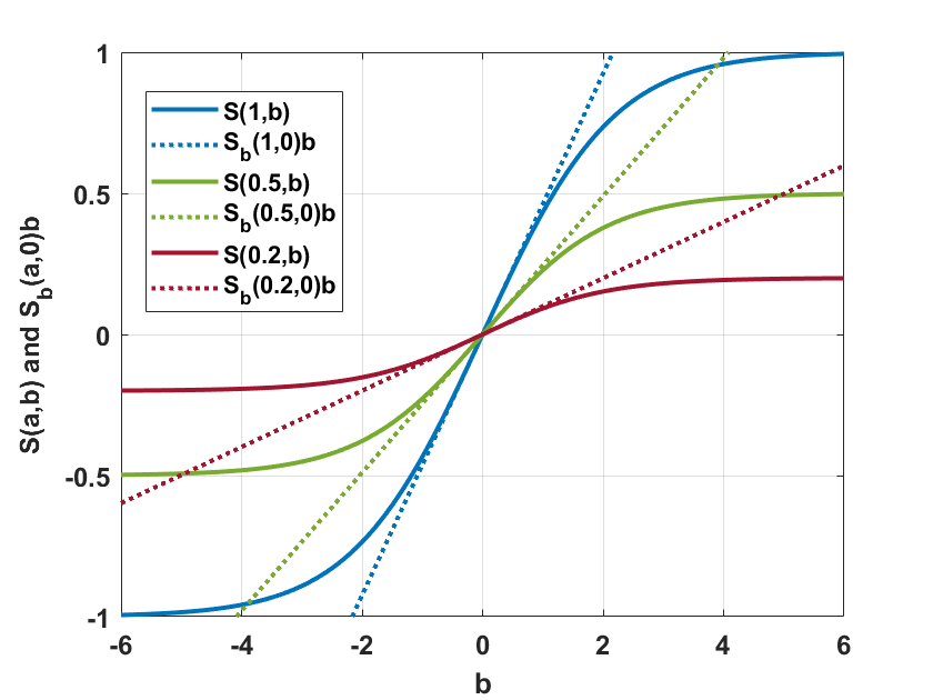
A closer look at (10) reveals that plays a role similar to the role of the sigmoid activation functions typically used in artificial neural networks [32]. In certain neural-network structures, each neuron generates an outcome by applying a bounded nonlinear transformation on the sum of its inputs received from other neurons in the network. This transfer function keeps the network stable by smoothening the neuron outcomes as well as by restricting them to reside between an upper and a lower bound. Consequently, the signals passed from one neuron to another become less sensitive to sharp variations in the inputs and the mapping learned by the network does not result in unbounded values for the variables of interest.
We propose to replace the nonlinear functions in the BP algorithm by linear ones. However, we design the proposed linear transformations in the network while taking into account the convergence condition of the distributed message-passing algorithm obtained. Having linear message-update rules in the BP algorithm enables us to analyze the network dynamics and develop effective optimization techniques to enhance system performance.
We realize the proposed linearization by approximating the message transfer function . Specifically, we use the first-order Taylor series expansion of with respect to its second argument, i.e., , where . This leads to a linear message-update rule as
| (12) |
where .
By applying this approximation on (10) and (11), while iterating the resulting linear message-update rule, we obtain
| (13) |
which shows that, given enough time, the overall result of the BP algorithm at a node is obtained, approximately, by a linear combination of all the local LLRs in the network. Note that we do not need the iteration index in this expression since (III) denotes the final result of the iterations.
Let denote a normed space where is defined and let denote a vector containing all the messages at iteration . A general message-passing algorithm is defined by where indicates the message-update rule. Convergence of such an iteration to a so-called fixed point means that the sequence obtained by iterating converges to a unique fixed point for any . Consequently, in (III) denotes (the decision variable made by) the fixed point of the linear BP algorithm in (12) and an approximation of (the decision variable made by) the fixed point attained via the BP in (10).
The linearization in (12) can be interpreted in two ways. One can see it as a linear approximation to the message-update rule in (10). Such an interpretation is valid since when ’s are Gaussian (which is a common practical case), one can normalize them without affecting the detection result. Specifically, when the decision variable follows a Gaussian distribution, for a constant false-alarm probability the probability of detection does not change by normalizing the decision variable. Consequently, by proper normalization of ’s, the messages can be made small enough to experience a linear behavior in the transfer functions.
Alternatively, one can opt not to normalize the local sensing outcomes and to consider (12) as a new message-update rule which is obtained directly by replacing the nonlinear transfer functions in the network by linear ones. Note that when the message values are too large to fall within the linear part of the transfer functions, the saturation behavior in acts as a thresholding process leading to a so-called hard fusion of the local LLRs. By using the linear transfer function in (12), the hard fusion rule is replaced by a soft one in which the sensing outcomes are directly combined without passing through that threshold. Since a soft fusion method outperforms a hard fusion one in general, one can expect a better overall detection result obtained by this linearization. A hard fusion scheme refers to a combination of binary-valued variables obtained by comparing the local sensing outcomes against (local) decision thresholds. See [33] for a comparison between the hard and soft decision methods.
Remark 1: Regardless of how (12) is interpreted, since the sigmoid functions are now removed, the linear transfer functions have to be designed properly to guarantee the convergence of the new message-update rule. We will discuss the convergence conditions in Section VI.
Remark 2: We have configured the linear combination in (III) such that it reveals the effect of the network topology on how the fusion coefficients are arranged. Specifically, for the one-hop neighbors of node we have one coefficient affecting the local likelihoods received, for the two-hop neighbors we have two coefficients and so on. We will use this observation in Section IV-B to develop a decentralized distributed inference method.
From (III) it is clear that, determining ’s for all in the network, based on a set of performance criteria, can be viewed as determining the values of ’s in the MRF. In [9, 5], the BP is designed and analyzed without directly considering the problem of fitting an MRF to the network behavior. Specifically, in those works, ’s are set by an empirical estimation of the correlations between the neighboring nodes in a window of time slots, i.e.,
| (14) |
where , referred to as the learning factor in this paper, is considered as a small constant and equals if is true and otherwise. denotes the number of samples used in this training process. We will see in Section VIII why should be small.
Such an approach does not directly take into account the impact of the learned factor graph on the system performance. In this paper, however, we argue that ’s provide extra degrees of freedom which can be used to optimize the system performance. Specifically, (10) shows that ’s determine the behavior of the transfer functions applied on the BP messages. Consequently, optimizing ’s can be viewed as finding an optimal set of transfer functions for the BP algorithm. Since we can normalize ’s without affecting the local detection performance, the proposed linear transfer functions are included in the feasibility region of this optimization. And, since a soft fusion method is better than a fusion method which clips the local LLRs, the performance of a BP iteration with the proposed linear transfer functions gives an upper bound on the detection performance of the BP algorithm defined by (10). Hence, by using linear transfer functions and by optimizing the resulting message-passing algorithm, we are optimizing the parameters of the BP algorithm in a distributed detection scenario.
Alternatively, note that the proposed linear BP algorithm defined by (12) is the same as the BP algorithm with (10) where ’s are large enough. And, ’s are the degrees of freedom in this design. Consequently, from an optimization perspective, there is no difference between the two message-passing algorithms.
IV Linear Fusion Based on Belief Propagation
In this section, we use the link between the BP and linear data-fusion to design distributed inference methods in both centralized and decentralized network configurations. In a centralized setting [14], there is a special node in the network, referred to as the fusion center (FC), which collects data from the sensing nodes, coordinates the distributed inference, and builds the overall inference outcome based on the collected data. In a decentralized (i.e., ad-hoc) network, however, there is no FC and the statistical inference is realized through the so-called peer-to-peer communication between the nodes.
IV-A Centralized Distributed Inference
Eq. (III) can compactly be stated as or, in matrix form, as
| (15) |
where , , and where . Assuming as the objective function corresponding to a certain application and as one of constraint functions indicating the requirements to be met by the system design, the optimal linear fusion in the network can be obtained by
| (P1) |
This is a generic linear fusion problem whose structure depends on the application at hand. We further clarify our points by considering a distributed spectrum sensing scenario where each node, say node , performs a binary hypothesis test on the decision variable to decide the availability of the radio spectrum.
In this scenario, is a binary-valued random variable representing the occupancy state of the radio spectrum where node is located. Let’s say, indicates that the spectrum band sensed by node is occupied whereas indicates the availability of that band for the secondary use. The signal samples used to form the test statistics at node can be expressed as
| (16) |
where denotes a zero-mean complex-valued Gaussian random variable which models the additive white noise at node while , also a zero-mean complex-valued Gaussian random variable, represents the signal transmitted by the th PU transmitter with . The channel gain from the th PU transmitter to node , denoted , is assumed constant during the sensing time interval. denotes a binary random variable which represents the state of the th PU transmitter, i.e., the th PU transmitter is on when and is off otherwise. is also assumed constant during the sensing time interval. According to this model, means that no PU signal is received at node , i.e., for all and the spectrum is available for the secondary use.
Given the state of , if we assume as in [9] that is a vector of i.i.d. complex Gaussian signal samples, then we have
| (17) |
where denotes the received signal-to-noise ratio (SNR) at node . Therefore, one needs to know the channel (power) gain, the transmitted signal power, and the noise level to obtain the probability distribution of .
In order to keep the resulting false-alarm rate below a predefined constraint , in [9] in (17) is replaced by
| (18) |
where is set such that , which leads to
| (19) |
This approach is practically appealing in the sense that, can be simply calculated in terms of the noise level and without the need for the channel gain and the transmitted power level.
The proposed structure remains intact if we use instead of (17). All other variables in (17) along with in (18) can be absorbed either into the coefficients in (III) or into the detection threshold . Consequently, we can justify here why the BP algorithm works well in [9] where energy detection is adopted as the local sensing method. As we show in Section VIII, in (18) works well only for small values of . We propose a new threshold adaptation scheme in Section V-B, which can always guarantee the false-alarm rate of the BP algorithm fall below a predefined upper bound without the need for any statistics other than the local noise level.
The performance of the binary hypothesis test discussed is formulated by the so-called false-alarm and detection probabilities defined, respectively, at node as and . The proposed transfer functions are linear and, given the status of ’s, our ’s are Gaussian random variables. Consequently, we can express the proposed system false-alarm and detection probabilities in closed form. These probabilities at node depend not only on the state of but also, in general, on the state of all other ’s being sensed throughout the entire network. We take these interdependencies into account by the total probability theorem. Specifically, at node and for we have
| (20) |
where , , and for , and . is the so-called -function. Note that contains all ’s except for . It is clear that and . By solving or we obtain a value for which guarantees the false-alarm or detection probability at node be, respectively, equal to or . The fact that is Gaussian comes from (III).
In a CR network, these parameters determine the secondary network throughput and the interference level caused on the PUs. Specifically, the higher the false-alarm probability the more vacant spectrum bands are mistakenly treated as occupied, leading to a loss in the network throughput. Consequently, the opportunistic spectral utilization of the th band is measured by . In addition, the higher the misdetection probability the higher the interference level imposed on the primary users. Hence, the interference level on the th band is measured by . In a rational design strategy, interference on PUs is associated with a cost.
We collect these performance metrics regarding the entire network in vectors and . Consequently, we can express the network performance by the following quantities
| (21) | |||
| (22) |
where denotes an all-one vector, denotes the aggregate network throughput calculated over all spectrum bands sensed across the whole network and denotes the aggregate interference caused on the PUs operating on those bands, where and while denotes the throughput achieved by using the th band. The cost of interference caused on the th band is denoted by which is included in .
Now, the optimal sensing performance is obtained by maximizing the aggregate system throughput subject to a constraint on the aggregate interference as well as the per channel false-alarm and misdetection constraints, i.e.,
| (P2) | |||
where and impose per-channel constraints on the false-alarm and misdetection probabilities. The sequential optimization method in [11], which maximizes the so-called deflection coefficient [34] of the detector, can be used to solve (P2) for a good suboptimal performance.
The deflection coefficient associated with is defined as
| (23) |
where, from (15), and . Hence, to maximize the deflection coefficients in the network, we only need and for all and . These statistics are clearly easier to obtain than , , and in (20).
Availability of the statistics discussed may require a centralized configuration in which an FC collects data from the nodes. As explained in [35, Sec. II-C], the standard preambles or synchronization symbols, which typically reside within the PU signals, can facilitate the estimation of the desired statistics in a centralized setting. In Section IV-B, we show how to optimize the system performance in a decentralized network and when those statistics are not available a priori.
Remark 3: Due to the nonlinearity of the message update rule in (10), the system false-alarm and detection probabilities are not available in closed form when the BP algorithm is used and, therefore, the performance optimization in (P2) or even guaranteeing a predefined level of performance in a BP-based system analytically is a very challenging task, if possible.
IV-B Decentralized Distributed Inference
Message-passing algorithms are of special interest in the decentralized network configurations where there is no FC, the communication between nodes is limited to one-hop neighbors, and, typically, there are no statistics available a priori regarding the wireless environment.
In order to build a decentralized distributed inference, we make three particular observations here. Firstly, note that for all . Moreover, as shown in Section VII, we can use ’s as the fusion coefficients, where , without affecting the detection probability obtained. Scaling down the coefficients is an effective method to mitigate the impact of graph cycles on the system performance.
Secondly, our MRF in (1) captures the correlations between the random variables by a set of pairwise links. In particular, if node is connected to node through node , the correlation between and is accounted for in (1) by two factors and multiplied together within . A similar process is observed in (III) where the impact of on , which depends on the correlation between and , is determined by multiplying two factors and corresponding, respectively, to the link from node to node and the link from node to node .
Thirdly, the fusion process in (III) is inherently symmetric. That is, each node performs the same local fusion on the data received from its neighbors and passes the result on along the path towards node . We use this symmetric structure, which is clarified in (24), to distribute the load of the desired optimization across all nodes in the network. Specifically, we assign each node the task of optimizing its own local fusion process. In this manner, each node has to deal with a few variables and with the statistics received from its one-hope neighbors only. The fact that makes this collection of localized optimizations a reliable distributed approach to the system performance optimization. The reason is that ’s received from neighbors with longer distance are multiplied by higher-order terms in the data-fusion process. Consequently, the system inherently favors, at each node, the data received from the close neighbors over the data from the more-distant ones.
| (24) |
Therefore, firstly, we further approximate (III) by keeping the first-order terms, i.e.,
| (25) |
We use , where , when optimizing the coefficients. In the vector form we have where contains all ’s such that and contains the local likelihood ratios at node and at all its neighbors.
Remark 4: The approximation in (25) is only used to realize the optimization of ’s in a decentralized configuration. The resulting coefficients are then used in a linear message-update rule as in (12). Hence, the overall impact of the distributed linear BP obtained is still approximated by (III).
Secondly, we optimize by considering the one-hop neighbors of node . In this manner, the correlation between and is captured in while the correlation between and is accounted for by . Hence, both of the correlations concerned are taken into account in the system design by the multiplication in (III) while each node sees its immediate neighbors only. This optimization can be performed conveniently in a distributed fashion since each node has to deal with only a few variables.
Contrary to the linear fusion method discussed in Section IV-A, here we have an iterative message-passing algorithm whose convergence needs to be guaranteed. In Section VI, we show that the convergence is guaranteed when we have which is a convex constraint on the coefficients. Therefore, the proposed decentralized linear fusion scheme is obtained by solving the following optimization at node , ,
| (P3) | |||
where , , and denote the application-specific local objective function, the local constraint functions, and the number of constraints at node , respectively. The major advantage of this optimization is that the local objective and constraint functions are calculated in terms of the statistics of and these statistics are now conveniently obtained due to the linearity of the proposed message update rule.
It is worth noting that, considering the overall system performance, the use of (25) does not mean that the impact of the higher-order terms on is ignored. Instead, the task of optimizing those terms are assigned to the other nodes in the network. It is clear that by this approximation we achieve a suboptimal solution. However, this solution distributes the optimization load well over the entire network by exploiting the symmetry in the overall data-fusion process achieved. Moreover, the use of (25) is supported by the observations made in [33] which investigates the performance of different fusion methods operating on erroneous data. In particular, it is shown in [33] that a soft fusion scheme is rather robust against the errors in the local test summaries reported by the cooperating nodes. Accordingly, we consider the impact of the truncation in (25) as a reporting error in the network and expect the system to tolerate it significantly. Taking advantage of this robustness in the linear fusion scheme, we break down the desired optimization into a set of small local optimizations which can be conducted collectively in a decentralized distributed setting. The numerical results in Section VIII support the effectiveness of the proposed optimization.
In the rest of the paper, we use to denote the coefficients in the linear approximation of the BP algorithm, i.e., , to distinguish those coefficients from the ones obtained by the proposed optimization. In addition, we use to contain all ’s such that .
In a spectrum sensing scenario, the proposed optimization is built by the well-known Neyman-Pearson hypothesis test [34] at each node. Specifically, at each node we aim at maximizing the detection probability subject to an upper bound on the false-alarm probability, i.e.,
| (P4) | |||
where and are derived, approximately, in a decentralized fashion as described in the following.
The conditional probabilities in (20), which govern the statistical behavior of the test summary at node , take into account any possible correlations between and all other ’s. Some nodes may, in fact, be located far away from node and their observations may have, if any, a little or negligible impact on the detection result at node . Hence, we simplify the calculations by limiting the summation in (20) to include only the correlations between and ’s observed by the one-hop neighbors of node . These statistics can be obtained by each node in a network with a decentralized configuration. The proposed approximation is expressed as
| (26) |
where is a vector which contains ’s with while for , we have and . Note that denotes the number of one-hop neighbors of node while and denote an estimation of the first- and second-order conditional statistics of the test summary at node given the value of and its immediate neighbors. And, is approximated as in (25).
Based on (25) we have and . Hence, the use of the deflection coefficient here can simplify the design even further compared to solving (P4). Maximizing the deflection coefficient is a classic low-complexity approach to optimal linear fusion which is considered in e.g., [10, 11, 12].
Remark 5: Since each node is typically connected to only a few neighbors, regardless of the scale of the network, each node has to deal only with a few variables when running the proposed optimization (and, as discussed later, when estimating the required statistics). Consequently, the scalability of the proposed detection scheme does not depend on the low-complexity optimization techniques in [10, 11, 12].
IV-C Discussion
The use of the BP algorithm, linear data-fusion, and MRFs in statistical inference systems cover a wide range of applications and design scenarios in the literature. However, these methods are normally investigated separately and in different contexts. In this paper, we intend to provide a more comprehensive view and shed light on the potential links between these effective tools. Therefore, we aim at presenting our ideas in an as generic of a framework as possible to help a reader possibly interested in a different application better understand the links discussed. The use of generic expressions to denote the objective and cost functions in (P1) and (P3) serves this purpose.
However, when interpreting the results of the proposed optimization framework, it should be noted that we focus on distributed detection in a wireless network. Consequently, some limitations may arise from the use of certain tools in this paper such as the type of the MRF model adopted or as the false-alarm and detection probabilities used to measure the system performance. Nevertheless, in the context of distributed detection, the models we use in this paper do not restrict the practicality of the design proposed. All the assumptions regarding the MRF, local sensing method, performance metrics, optimization scenarios, availability of channel statistics, network configuration, and the possibility of one-hop communications, etc. are in line with the design scenarios widely-used in the literature.
In fact, the proposed distributed optimization is based on the linear fusion structure in (III) and its symmetric nature as clarified in (24). The linear fusion discussed is mainly based on (1) and (4) which together build a relatively generic model for a distributed binary hypothesis test. Due to the reasons discussed in Section II, modeling the joint pdf of the variables in terms of pairwise correlations as in (1) is a commonly-used approach in distributed detection. In addition, the use of an exponential form in (4) to model the behavior of correlated binary-valued random variables is a popular choice since, first, it is supported by the principle of maximum entropy [15] and, second, when the graphical model is built in terms of products of functions, these products turn into additive decompositions in the log domain.
The use of the false-alarm and detection probabilities, as performance metrics, only affects the structure of the objective and constraint functions discussed. As clarified in Remark 5, when using the proposed distributed optimization, each deals with a relatively small optimization problem and, therefore, the type of the objective and constraint functions in (P4) are not of major concern. Hence, we do not lose the generality of the proposed distributed optimization by the use of these metrics. Our main goal in such formulations is to facilitate the design of the CR network since the false-alarm and detection probabilities are directly linked to the CR network throughput and the level of interference experienced by the PUs, respectively. This link is explained in Section IV-A.
V Blind Distributed Detection
We propose the notions of adaptive linear belief propagation and detector calibration here to realize a near-optimal distributed detection performance when there is no information available a priori regarding the statistical behavior of the radio environment.
V-A Offline Learning and Optimization
As we saw in Section IV, in order to optimize the fusion weights in the proposed linear message-passing algorithm, we need the first- and second-order statistics of the local sensing outcomes. Since we do not assume any prior knowledge about the channel statistics or the behavior of the PUs, we have to estimate those parameters based on the detection outcome. This is a challenging task since the detection outcome itself depends on those estimates. Erroneous detection outcomes lead to erroneous estimates of the desired statistics which, in turn, deteriorate the detection results. We overcome this challenge by implanting an adaptation process within the linear BP algorithm, which is run offline on a set of data samples collected and processed for channel estimation and detector optimization purposes. This adaptation is realized by an offline linear BP algorithm whose outcome is a set of near-optimal coefficients used in the main linear BP algorithm which is responsible for spectrum sensing in real time.
In a blind detection scheme the only source of information is the detector outcome. Hence, we have to use and to estimate and for all for all . These estimates are erroneous in nature due to the non-zero false-alarm and misdetection probabilities in the system. As an example note that, to estimate node needs to calculate an average over the samples of received when . However, node does not exactly know when and it can only calculate . When the sensing outcome indicates , it may be, in fact, a misdetection and including the sample in the averaging process may lead to a significant error in that case. Note that samples can vary widely in size depending on the status of . Similar errors can also occur due to the false-alarm incidents.
Therefore, we need to enhance the quality of sensing in order to have high-quality estimates of the desired statistics which, in turn, are used to achieve a better sensing quality. Clearly, we are facing a loop here. Hence, we design an iterative learning-optimization loop to optimize the proposed message-passing algorithm. This loop works as an offline linear BP algorithm which operates on a window of samples of .
In the following, we use (instead of ) to denote the iteration index of the offline linear BP algorithm in order to distinguish this iteration from the main linear BP algorithm. In addition, we use to denote a window of samples of stored for the proposed offline data processing and to denote the offline sensing outcomes, while we use and to denote respectively the fusion coefficients and the detection threshold at node at (offline) iteration . For notational convenience, we do not explicitly show the timing of the samples here. However, it should be noted that by and we are referring, respectively, to samples of and corresponding to . It is also worth noting the difference between and . Throughout the paper, we use to denote the sensing outcomes resulted from the main linear BP. However, is used here to denote the offline sensing outcomes based on which the desired statistics are estimated.
| Adaptive Linear Belief Propagation for Detector Optimization |
| Input: , , , |
| Output: Near-optimal coefficients for linear BP |
| 1. Let and initialize by comparing against ; |
| 2. while |
| 3. for node |
| 4. Calculate and for all ; |
| 5. Solve (P4) to find coefficients and threshold ; |
| 6. end |
| 7. Run the resulting linear BP on to find ; |
| 8. ; |
| 9. end |
| 10. for node |
| 11. for |
| 12. if |
| 13. ; |
| 14. else |
| 15. ; |
| 16. end |
| 17. end |
| 18. end |
| 19. Output for ; |
Algorithm I provides a pseudo-code of the proposed adaptation algorithm in which per-node computations are clarified. The adaptation is designed in a way that each node processes samples of only from its immediate neighbors. Hence, in the proposed distributed optimization no further information is used at each node other than those assumed available in [9].
The loop starts with initializing by the local sensing process on . Specifically, for , initial offline sensing outcome is created at node by comparing against the corresponding local threshold calculated by (19) which only requires the noise variance. The noise levels can be measured in practice [9]. At iteration , all samples of are used to calculate and for all , . These estimates are then fed into (P4) to find the coefficients and thresholds . The resulting linear BP is then run over to find . The iteration stops after either a predetermined number of cycles or when there is no significant change in the updated parameters and statistics concerned. Lines 1 to 9 in Algorithm I describe this iteration.
Due to the multipath fading or shadowing effects typically associated with the wireless environment, we may experience very low SNR levels at some sensing nodes. In such cases, the signals to be detected may be buried under a heavy noise and the channel estimation process may not be able to reliably capture the correlations between the desired random variables. In order to ensure that the system performance is not degraded in such conditions – to below the performance level of the BP algorithm – we compare the coefficients obtained by the adaptive linear BP against their counterparts in the linearized version of the main BP algorithm. If a coefficient obtained by the offline iteration is too small compared to its counterpart in the main BP, then that coefficient is not used in the adaptation and the one from the main BP is used instead. Lines 10 to 18 in Algorithm I illustrate this process. Specifically, if is greater than a predefined value denoted by , then is used as the final fusion weight. Otherwise, is used. The final coefficients , , are then used in the main linear BP algorithm for spectrum sensing.
The proposed adaptation scheme enables us to rely on the effectiveness of the BP algorithm in capturing the interdependencies of the random variables in low SNR regimes while enhancing its performance by the linear fusion techniques whenever there is a room for such an enhancement. This is a hybrid design in which the two detection techniques work together. The BP algorithm properly takes into account the outcome of the nodes in low SNR conditions while the linear fusion enhances the performance by injecting more information about the environment into the BP algorithm and this information is obtained from the nodes operating in better conditions. It is reasonable to assume that different nodes operate in different conditions due to the inherent spatial diversity in a wireless network.
It is worth noting that, the time is modeled as slotted in this paper and we refer to the proposed adaptation process as offline to distinguish it from the main linear BP algorithm which is executed at the beginning of every time slot. Unlike the main linear BP iteration (or the legacy BP), Algorithm I is not run at every time slot. Instead, it is executed with a longer periodicity and in step with the changing characteristics of the radio environment. Since we assume that the statistical behavior of the environment changes slowly, the period over which Algorithm I is repeated is much longer than the time-slot duration. Specifically, if the spectrum sensing is performed at , , with being the slot duration, then Algorithm I is executed at for , while . Moreover, this adaptation is based on a window of data samples generated in the past compared to the data samples used for spectrum sensing. Hence, with respect to the spectrum sensing process, the fusion coefficients are adapted offline.
Remark 6: Since the statistics of the radio environment change slowly compared to the instantaneous status of ’s, the proposed adaptation is run far less frequently than is the main linear BP algorithm. Consequently, the proposed learning-optimization scheme does not lead to any significant increase in the computational complexity or communication overhead of the existing BP-based distributed detection methods.
We do not use to set the detection thresholds in the main linear BP algorithm. The reason is that, to guarantee a certain level of the false-alarm or misdetection probability in the system we need a more accurate threshold adaptation mechanism. In the following, we propose a blind threshold adaptation scheme which guarantees the required performance.
V-B Detector Calibration
As discussed in Section V-A, when we rely only on the detector outcome to derive the required conditional probabilities and statistics, we have to deal with inevitable errors. And, by evaluating (20) and (26) we realize that the threshold values aimed at guaranteeing a certain false-alarm or detection probability appear to be too sensitive to these errors. Specifically, we have found through computer simulations that when , , and in (20) or , , and in (26) are estimated solely based on the detection outcomes, i.e., without prior knowledge about the joint statistical behavior of ’s, the thresholds obtained by or cannot always guarantee the desired performance levels. However, they work well when the required statistics are available.
Hence, we need a blind threshold adaptation method. We develop such an adaptation here by showing that the desired thresholds can be found through evaluating the outcomes of two sensing schemes which work in the same environment. It is clear that the sensing outcomes are always available and can be measured with no error. In this design, we use the fact that if the false-alarm (misdetection) probability of a sensing method can be set arbitrarily, that sensing method can be used to find a proper detection threshold for a better sensing scheme whose false-alarm (misdetection) probability needs to be below a certain level.
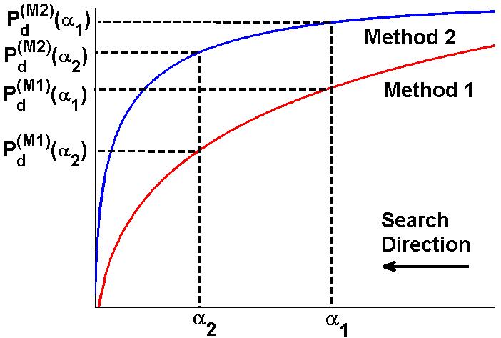
To clarify this observation, see Fig. 2 in which the receiver operational characteristic (ROC) curves of two hypothetical sensing methods, Method 1 and Method 2, are depicted. Both methods are used to decide whether a binary-valued variable of interest, denoted here by , equals 1. We assume that Method 2 exhibits a better performance and that we can set the detection threshold in Method 1 such that its false-alarm probability is fixed at . Let denote that threshold. When is adopted for Method 1, the probability of observing 1 as the outcome of Method 1 can be stated as
| Pr | ||||
| (27) |
where denotes an estimation of given by Method 1 (i.e., the outcome of Method 1), and , while and denote, respectively, the false-alarm and detection probabilities of Method 1. denotes the detection probability of Method 1 when its false-alarm probability equals . In the following, we use similar notations regarding Method 2.
can be measured in a simple fashion. We just need to count the number of times equals 1 over a long enough period of time. Now, let denote the detection threshold in Method 2. We are looking for at which . We start with and gradually increase the threshold level. At the starting point, Method 2 gives only 1 as its outcome. The reason is that when , we have . Hence, at the beginning . It is also clear that, at the beginning we have .
By increasing both values of and decrease reducing the gap between and . We stop the search when the two values coincide which happens when we have and . When the gap is zero we have . This leads to . Therefore, now we have found a detection threshold which guarantees while .
The proposed threshold adaptation is based on measuring the difference in the behaviors of two sensing schemes operating in the same environment. Therefore, we refer to this process as the calibration of Method 2 by using Method 1.
Remark 7: Assuming no prior knowledge about the environment means that none of the following probabilities are (perfectly) available: , and . The proposed calibration finds the desired threshold level without the need for any of those parameters.
In our spectrum sensing system, we have two options to use for calibrating the linear BP algorithm. The first option is the local sensing performed at each node. And the second one is the legacy BP-based distributed detection when the required false-alarm probability is small. In both of those detection schemes, we can guarantee a predefined level of false alarm only by knowing the noise level at each node. As mentioned before, the noise levels can be measured in practice. Since a linear BP with near-optimal coefficients exhibits a better performance level than the level shown by either of those methods, either of them can be used to calibrate the linear BP. We use the first option not to be limited to a small value of .
VI Convergence Conditions
An iterative message-passing algorithm which is run on a general factor graph does not necessarily converge to a fixed point. Even in case of the BP, when the graph contains loops, there is no guarantee, in general, that the beliefs will approximate the true marginals or even will converge to a fixed point at all. Furthermore, by using the proposed linear approximation in (12) we remove the nonlinear transfer functions and, consequently, increase the sensitivity of the nodes’ outcomes to their input. Moreover, we increase the dynamic range of the values messages can attain. This change in the structure of the BP algorithm may deter its stability and convergence. However, by a careful design of the linear transformations, we can guarantee the convergence to a fixed point. In addition, by using the proposed optimizations we can enforce the algorithm to converge to a certain fixed point which leads to the desired performance. To realize this goal, we need to guarantee the so-called contraction mapping condition [36, 4] of the overall transformation obtained.
We collect all the messages , in the vector . Then, we can express the message-update rule (10) in matrix form as and the linear approximation as where denotes an matrix which contains ’s while denotes the offset in this transformation. Assuming that the th and th elements of are, respectively, and , we have
| (28) |
Recall from Section III that, we denote a general message-update rule as where . From [4, Theorem 1] we know that if there exist such that for any , then the sequence convergence is guaranteed. This is known as the contraction condition. Moreover, for a differentiable mapping , for any point on a segment between and denoted by we have . Therefore, the following condition guarantees the convergence of a message passing algorithm defined by
| (29) |
For simplicity, we work with the matrix norm . By using the the proposed linear approximation in (12), we have which leads to . Consequently, the contraction condition holds if which, according to (28), is equivalent to which can be restated as which is equivalent to where indicates the number of neighbors of node . Therefore, by imposing the following constraint on the proposed optimizations we guarantee the convergence of the proposed linear message-passing algorithm
| (30) |
This is a convex constraint and does not add any significant challenge to the optimization problems at hand.
It is worth noting that, (30) is the last piece we need to develop an optimization framework for the BP-based distributed inference systems, which takes the advantages of both the BP and linear fusion. In particular, the BP algorithm is an effective approach to take into account the correlations between a group of spatially-distributed nodes while linear fusion is known to enable building low-complexity optimal decision variables based on the data exchanged between such nodes. By combining these capabilities, we develop a message-passing algorithm which takes into account the impact of pairwise correlations in accordance with the MRF model and is easy to optimize while its convergence is guaranteed.
VII Impact of cycles
Depending on the network topology, the factor graph may contain cycles (loops) which might affect the quality of the marginals obtained by a message-passing algorithm. It is known that the presence of cycles in the graph can lead to the overconfidence in the beliefs which may degrade the system performance [9]. The impact of cycles can be mitigated by using the so-called tree-reweigthed-BP (TRW-BP) algorithm [5]. This method reduces the amount of information exchanged between the nodes to maintain an acceptable performance level when the factor graph contains cycles.
In the TRW-BP the message from node to node is given by
| (31) |
while the beliefs are built as
| (32) |
where ’s are referred to as the edge appearance probabilities (EAP). In this method, we have and the BP algorithm is a special case of the TRW-BP with for all . Using smaller values for EAPs reduces the impact of cycles at the expense of cooperation between the sensing nodes. The performance of the TRW-BP can be optimized over the EAPs. However, this optimization grows rapidly in size with the number of nodes making it difficult to solve in a distributed manner. Assuming the same EAPs for all the links, i.e., for all , shrinks the problem into a scalar optimization which can easily be solved in a distributed setting. The resulting method, which is referred to as uniform TRW-BP (UTRW-BP) algorithm, can achieve a good level of resistance against the impact of cycles in the graph. It is shown in [5] that the optimal EAP is given by
| (33) |
where is the average degree of the graph, i.e., the average number of connections of the nodes in the network. We know that, can be computed in a decentralized architecture by an average consensus algorithm.
Following the same approach as in Section III, we express the messages and the decision variables achieved by the UTRW-BP as
| (34) | ||||
| (35) |
which show that at every iteration the messages hit a damping factor before being combined together to from a new message or decision variable. And, the decision variable at node approaches approximately to
| (36) |
where .
From (VII) we obtain some interesting observations. In particular, we observe a stronger decaying effect by distance from node than we had before. As we saw in (III), since , the impact of other nodes on decreases by the distance of those nodes from node . Now, this decaying is stronger and in favor of the one-hop neighbors even more than before. Specifically, if arrives at node through a path of length , then it is multiplied by in the data-fusion process. Consequently, in the presence of loops, i.e., when there is more than one path from node to node , the impact of on received through the shortest path is amplified compared to the ones received through the other paths. In other words, in the UTRW-BP the decision variable at a node is built mainly by the data received through the tree sub-graph(s) connecting that node to all the other nodes via the shortest paths. Hence, reduces the overconfidence in nodes by alleviating the impact of cycles.
We can accommodate this decaying effect in the proposed linear BP scheme. Note that, for a fixed false-alarm probability the detection probability is positively homogeneous of degree zero with respect to . To show this we set the detection threshold in (26) as
| (37) |
where . Consequently, and
| (38) |
where .
Now we see that by using instead of as the fusion vector at node , the detection probability remains unchanged. The reason is that, the variables and are all multiplied by , thus, canceling the effect of this scaling on . Since the detection probability is a monotonically increasing function of the false-alarm probability, the global optimum in (P4) occurs when . Therefore, given as a solution for (P4), its scaled version is also a global optimum. Hence, by using in (12) we obtain a similar decaying effect to the one observed in UTRW-BP without altering the proposed optimization framework. Note also that, using the deflection coefficient as the objective function in the proposed distributed optimization does not affect this argument since the deflection coefficient is a homogeneous function of as well.
As the final point, note that when the number of iterations is small there is no need to be concerned of the impact of cycles [9].
VIII Numerical Results
Fig. 3 depicts the network configuration used in our simulations. We consider two PU transmitters and five sensing nodes as SUs. Nodes 1 and 2 are located within the range of PU transmitter 1, nodes 4 and 5 are located within the range of PU transmitter 2, while node 3 is located within the range of the both PU transmitters. These nodes exchange messages with each other over a set of wireless links, depicted as the dashed lines in the figure, to conduct a distributed detection scheme through which the transmission opportunities are discovered within the spectrum bands allocated to the PUs.
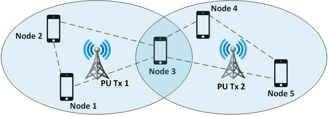
Energy detection is used as the local detection method at each node with samples to estimate the received signal energy. The SNR levels of the signals received at nodes 1 and 5 are -5 dB, at nodes 2 and 4 are -8 dB and at node 3 are -10 and -10 dB. We realize a spatially-correlated occupancy pattern by making the primary transmitters exhibit correlated random on and off periods. This is an extension of the simulation scenario in [9] where one of the PU transmitters is constantly on while the other one is off all the time. The channel coefficients are constant during the sensing period as in [9]. The number of iterations is 3 for all the message-passing algorithms considered in this section. In addition, the offline BP algorithm is repeated only 4 times, i.e., . Each data point in the simulation results is obtained by averaging the detection outcomes over 20,000 time slots. A window of time slots is used to train all the message-passing algorithms.
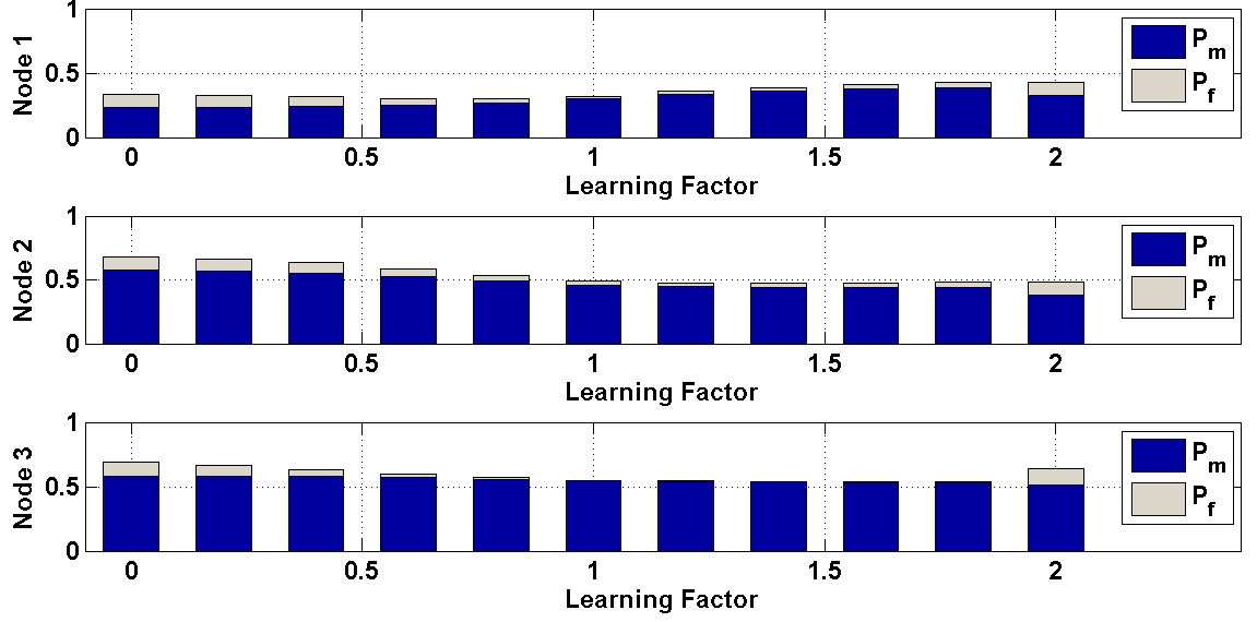
Fig. 4 depicts the system performance in terms of the false-alarm and misdetection probabilities vs. the learning factor in (14). We observe different performance levels for different values of the learning factor, which indicates the need for optimization. To cover a wide range of possible performance levels of the BP algorithm, we adopt three values as . As reported in [9], the BP algorithm works better when the learning factor is small. However, note that how to determine the best value for is unknown. For the sake of brevity, we only focus on nodes 1, 2, and 3. Nodes 4 and 5 experience similar conditions as those in which nodes 1 and 2 operate. The optimal linear fusion scheme is realized in this section by solving (P2) via the sequential optimization method described in [11].
We use ROC curves to demonstrate and compare the detection performance achieved by the different methods. In Fig. 5(a) we see the performance of node 1 which operates under a relatively better SNR regime than those experienced by nodes 2 and 3. The performance of the proposed linear BP along with those of the optimal linear fusion and the local detection are shown for comparison. We first observe that the performance of the BP algorithm improves by increasing the value of from 0.2 to 0.6 and then degrades by a further increase in . Moreover, we observe that both the BP with and the proposed linear BP achieve the performance of the optimal linear fusion scheme without any prior knowledge available concerning the radio environment. In comparing these performance results it should be noted that, firstly, is found by a numerical search and secondly, as it is shown later in this section, it fails to always guarantee the performance constraint on the system false-alarm probability. The proposed method achieves the optimal performance blindly while guaranteeing that the required constraint on the false-alarm probability is always met.
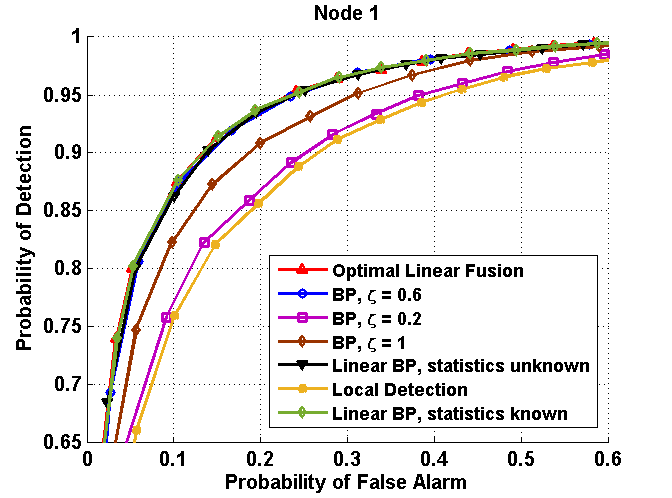
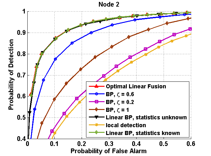
Fig. 5(b) depicts the detection performance obtained at node 2. Here we have a clear performance gap which illustrates that the proposed method outperforms the conventional BP algorithm. Therefore, we can see that when operating under a lower SNR level (than the one observed in node 1), the proposed linear BP achieves the detection rate of the optimal linear fusion while the BP algorithm falls behind. This can be attributed to the better learning capability and also to the better combination of the local test summaries in the proposed linear BP algorithm. Specifically, we know that a properly designed linear fusion scheme provides a constructive discrimination [37] on the local sensing outcomes when they are combined together to build a decision variable. This discrimination alleviates the degrading effect of the local sensing results obtained in low SNR regimes by emphasizing the effect of the ones created by the more reliable nodes. In Fig. 5(b), it appears that such discrimination is better realized in the proposed linear BP algorithm compared to the conventional BP. Note that, both methods use the same data which is obtained through the exchange of information between the one-hop neighbors in the network.
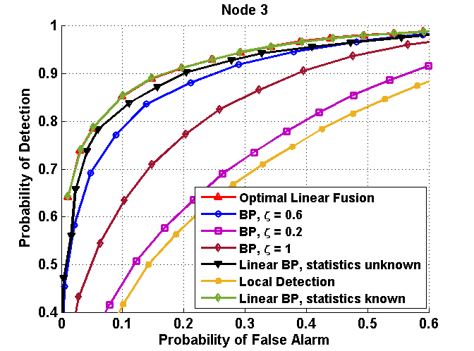
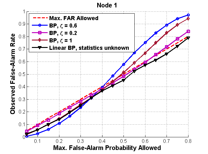
Fig. 6(a) depicts the detection performance of node 3. Again, we see that the optimal linear BP outperforms the conventional BP algorithm. And, the linear BP nearly attains the detection rate of the optimal linear fusion scheme without having any prior knowledge about the radio environment.
By comparing the performance gap between the local detection scheme and all other distributed detection methods considered in this section we see that the impact of a distributed detection scheme is more significant when the nodes operate in low SNR regimes and that is the situation in which the proposed method offers a higher performance gain than what is achieved by the conventional BP algorithm. In other words, in a network of distributed sensors, when the SNR levels are low we have a stronger need to establish some sort of cooperation between the sensing nodes to achieve more-reliable sensing results and the linear BP algorithm offers a more significant gain, over the other methods, in such a condition.
The performance of the proposed detector calibration method is depicted in Fig. 6(b) where the false-alarm rate (FAR) observed is depicted vs. the constraint imposed on the system false-alarm probability. We see that when the detection threshold is determined by the proposed calibration, the FAR is always guaranteed to fall below the predefined upper bound. However, when the conventional BP is used with the detection threshold calculated by (19), it fails to achieve the required performance guarantees when the constraint is not small enough. Equivalently, Fig. 6(b) shows that, when (19) is used, to achieve the required performance guarantee for an arbitrary , we have to keep the learning factor relatively small. However, as we saw previously by inspecting the ROC curves, when is small the detection performance is far from optimal. Hence, the proposed linear BP algorithm outperforms the existing BP algorithm when the FAR of the system is required to be controlled.
It is worth noting that, the use of (18) is inspired by (17) which is derived assuming that if , then is a vector of Gaussian random variables. However, this is not always the case. From (16) we see that, when there exist more than one PU transmitter, as in our network configuration, cannot be assumed necessarily to follow a Gaussian distribution. Consequently, the violation of the FAR constraint when is used appears to be due to the error in modeling the statistical behavior of . The proposed calibration method works based on modeling the behavior of , given , by a Gaussian distribution which is, in fact, the case. Therefore, the proposed system is capable of meeting the required FAR constraint.
As the final point, the better performance of the proposed threshold adaptation scheme does not stem from the linearity of the proposed message-passing algorithm since the calibration method proposed does not depend on the behavior of the transfer functions affecting the messages. For the sake of brevity, Fig. 6(b) depicts only the FAR observed at node 1. All other nodes show a similar performance.
IX Conclusions
We demonstrated that a BP algorithm in a network of distributed agents can be viewed or approximated as a distributed linear data-fusion scheme. Accordingly, we addressed two particular issues in using the BP algorithm for distributed detection: First, the lack of knowledge about the statistical behavior of the BP messages exchanged between the nodes and second, the lack of a proper threshold adaptation mechanism in a BP-based detection scheme.
Regarding the first issue, our analysis and simulation results demonstrate that, when the local sensing results follow the Gaussian distribution,
-
•
In a centralized configuration and when the first- and second-order statistics of the local detection results of all nodes are available at the FC, a linear fusion of all the local detection results, realized by (P1), can obtain the desired performance and there is no need for an iterative message-passing algorithm.
-
•
In a decentralized configuration and when at each node the first- and second-order statistics of the local detection results of its one-hop neighbors are available, the desired performance can nearly be obtained via a linear message-passing algorithm realized by (P3).
-
•
In a decentralized configuration and when there is no statistics available a priori, the desired performance can be obtained via a linear message-passing algorithm in which the weighting coefficients are obtained blindly via the offline adaptive linear BP algorithm described in Section V-A.
And, regarding the second issue, we have shown that in the proposed linear BP algorithm,
-
•
The detection threshold to guarantee a certain false-alarm (or misdetection) probability can be found analytically at each node when the first- and second-order statistics of the one-hop neighbors of that node are available.
-
•
The system false-alarm (or misdetection) probability can be guaranteed to fall below a certain level by the calibration method proposed in Section V-B without the need for any statistics describing the behavior of the local test summaries or the wireless environment.
References
- [1] F. R. Kschischang, B. J. Frey, and H. . Loeliger, “Factor graphs and the sum-product algorithm,” IEEE Transactions on Information Theory, vol. 47, no. 2, pp. 498–519, Feb 2001.
- [2] N. Noorshams and M. J. Wainwright, “Stochastic belief propagation: A low-complexity alternative to the sum-product algorithm,” IEEE Transactions on Information Theory, vol. 59, no. 4, pp. 1981–2000, April 2013.
- [3] H. . Loeliger, “An introduction to factor graphs,” IEEE Signal Processing Magazine, vol. 21, no. 1, pp. 28–41, Jan 2004.
- [4] J. M. Mooij and H. J. Kappen, “Sufficient conditions for convergence of the sum-product algorithm,” IEEE Transactions on Information Theory, vol. 53, no. 12, pp. 4422–4437, Dec 2007.
- [5] H. Wymeersch, F. Penna, and V. Savic, “Uniformly reweighted belief propagation for estimation and detection in wireless networks,” IEEE Transactions on Wireless Communications, vol. 11, no. 4, pp. 1587–1595, 2012.
- [6] A. Y. Lokhov, M. Vuffray, S. Misra, and M. Chertkov, “Optimal structure and parameter learning of Ising models,” Science advances, vol. 4, no. 3, p. e1700791, 2018.
- [7] Z. Zhang, Z. Han, H. Li, D. Yang, and C. Pei, “Belief propagation based cooperative compressed spectrum sensing in wideband cognitive radio networks,” IEEE Trans. Wireless Commun., vol. 10, no. 9, pp. 3020–3031, Sep. 2011.
- [8] H. Li, “Cooperative spectrum sensing via belief propagation in spectrum-heterogeneous cognitive radio systems,” in 2010 IEEE Wireless Communication and Networking Conference, April 2010, pp. 1–6.
- [9] F. Penna and R. Garello, “Decentralized Neyman-Pearson test with belief propagation for peer-to-peer collaborative spectrum sensing,” IEEE Transactions on Wireless Communications, vol. 11, no. 5, pp. 1881–1891, May 2012.
- [10] Z. Quan, S. Cui, and A. H. Sayed, “Optimal linear cooperation for spectrum sensing in cognitive radio networks,” IEEE J. Sel. Topics Signal Process., vol. 2, no. 1, pp. 28–40, Feb. 2008.
- [11] Z. Quan, S. Cui, A. H. Sayed, and H. V. Poor, “Optimal multiband joint detection for spectrum sensing in cognitive radio networks,” IEEE Trans. Signal Process., vol. 57, no. 3, pp. 1128–1140, March 2009.
- [12] Z. Quan, W. Ma, S. Cui, and A. H. Sayed, “Optimal linear fusion for distributed detection via semidefinite programming,” IEEE Trans. Signal Process., vol. 58, no. 4, pp. 2431–2436, 2010.
- [13] G. Taricco, “Optimization of linear cooperative spectrum sensing for cognitive radio networks,” IEEE J. Sel. Topics Signal Process., vol. 5, no. 1, pp. 77–86, Feb. 2011.
- [14] I. F. Akyildiz, B. F. Lo, and R. Balakrishnan, “Cooperative spectrum sensing in cognitive radio networks: A survey,” Physical Commun., vol. 4, no. 1, pp. 40–62, March 2011.
- [15] M. J. Wainwright, M. I. Jordan et al., “Graphical models, exponential families, and variational inference,” Foundations and Trends in Machine Learning, vol. 1, no. 1–2, pp. 1–305, 2008.
- [16] N. Wiberg, Codes and decoding on general graphs, 1996.
- [17] S.-Y. Chung, T. J. Richardson, and R. L. Urbanke, “Analysis of sum-product decoding of low-density parity-check codes using a Gaussian approximation,” IEEE Trans. Inf. Theory, vol. 47, no. 2, pp. 657–670, 2001.
- [18] T. J. Richardson, M. A. Shokrollahi, and R. L. Urbanke, “Design of capacity-approaching irregular low-density parity-check codes,” IEEE Trans. Inf. Theory, vol. 47, no. 2, pp. 619–637, 2001.
- [19] S. Ten Brink, “Iterative decoding trajectories of parallel concatenated codes,” in 3rd IEEE ITG Conf. Source and Channel Coding, 2000, pp. 75–80.
- [20] ——, “Rate one-half code for approaching the Shannon limit by 0.1 dB,” Electronics letters, vol. 36, no. 15, pp. 1293–1294, 2000.
- [21] H. El Gamal and A. R. Hammons Jr., “Analyzing the turbo decoder using the Gaussian approximation,” in Proc. Int. Symp. Information Theory. IEEE, 2000, p. 319.
- [22] ——, “Analyzing the turbo decoder using the Gaussian approximation,” IEEE Trans. Inf. Theory, vol. 47, no. 2, 2001.
- [23] M. Welling and Y. W. Teh, “Linear response algorithms for approximate inference in graphical models,” Neural computation, vol. 16, no. 1, pp. 197–221, 2004.
- [24] M. Bayati and A. Montanari, “The dynamics of message passing on dense graphs, with applications to compressed sensing,” IEEE Trans. Inf. Theory, vol. 57, no. 2, pp. 764–785, 2011.
- [25] D. L. Donoho, A. Maleki, and A. Montanari, “Message-passing algorithms for compressed sensing,” Proceedings of the National Academy of Sciences, vol. 106, no. 45, pp. 18 914–18 919, 2009.
- [26] ——, “Message passing algorithms for compressed sensing: I. motivation and construction,” in IEEE Information Theory Workshop (ITW 2010). IEEE, 2010, pp. 1–5.
- [27] S. Rangan, “Generalized approximate message passing for estimation with random linear mixing,” arXiv preprint arXiv:1010.5141, 2010.
- [28] ——, “Generalized approximate message passing for estimation with random linear mixing,” in Int. Symp. Inf. Theory Proceedings. IEEE, 2011, pp. 2168–2172.
- [29] V. Toto-Zarasoa, A. Roumy, and C. Guillemot, “Maximum likelihood BSC parameter estimation for the slepian-wolf problem,” IEEE Communications Letters, vol. 15, no. 2, pp. 232–234, 2010.
- [30] F. Penna, R. Garello, and M. A. Spirito, “Likelihood-ratio propagation and consensus in wireless networks with markov random field models,” in 2010 IEEE Globecom Workshops. IEEE, 2010, pp. 1259–1263.
- [31] ——, “Distributed inference of channel occupation probabilities in cognitive networks via message passing,” in 2010 IEEE Symposium on New Frontiers in Dynamic Spectrum (DySPAN). IEEE, 2010, pp. 1–11.
- [32] K. Gurney, An introduction to neural networks. CRC press, 1997.
- [33] S. Chaudhari, J. Lunden, V. Koivunen, and H. V. Poor, “Cooperative sensing with imperfect reporting channels: Hard decisions or soft decisions?” IEEE Trans. Signal Process., vol. 60, no. 1, pp. 18–28, Jan. 2012.
- [34] S. M. Kay, Fundamentals of statistical signal processing. Prentice Hall PTR, 1993.
- [35] P. Paysarvi-Hoseini and N. Beaulieu, “Optimal wideband spectrum sensing framework for cognitive radio systems,” IEEE Trans. Signal Process., vol. 59, no. 3, pp. 1170–1182, March 2011.
- [36] C. Huang, Y. Li, and L. Dolecek, “Belief propagation algorithms on noisy hardware,” IEEE Transactions on Communications, vol. 63, no. 1, pp. 11–24, Jan 2015.
- [37] Y. Abdi and T. Ristaniemi, “Random interruptions in cooperation for spectrum sensing in cognitive radio networks,” IEEE Transactions on Communications, vol. 65, no. 1, pp. 49–65, 2017.