Mixed QCD$\otimes$QED corrections to on-shell $Z$ boson production at the LHC

Abstract

We compute the mixed QCD$\otimes$QED corrections to the production of on-shell $Z$ bosons at the LHC at a fully-exclusive level. We also include the factorised NLO QCD correction to $Z$ boson production and NLO QED correction to $Z$ boson decay into two leptons. We make use of an abelianised version of the nested soft-collinear subtraction formalism to perform this computation. We study the phenomenological impact of the mixed QCD$\otimes$QED corrections for a number of observables relevant for LHC phenomenology.

1 Introduction

The recent years have seen a transition of the Large Hadron Collider (LHC) from a discovery machine to a precision machine. The reason for this is the absence of a direct observation of New Physics which, even after the discovery of the Higgs boson Aad:2012tfa ; Chatrchyan:2012xdj , is needed to clarify questions left open by the Standard Model. Forthcoming searches for physics Beyond the Standard Model (BSM) will focus on systematic studies of possible small deviations from Standard Model predictions in precision observables. A reliable theoretical description of such observables within the Standard Model is an important prerequisite for the success of this research program.

A case in point is the hadronic production of charged leptons via a virtual photon and/or the $Z$ boson, the celebrated Drell-Yan (DY) process Drell:1970wh (see Mangano:2015ejw for a review). Its high production rate and distinct signature make it extremely useful for luminosity monitoring Dittmar:1997md ; Khoze:2000db ; Giele:2001ms and detector calibration Haywood:1999qg . Being theoretically well-understood, this process is also suited for electroweak (EW) precision physics, such as the measurement of the weak mixing angle Haywood:1999qg ; Sirunyan:2018swq . Moreover, DY production is used in parton distribution function (PDF) fits Harland-Lang:2014zoa ; Ball:2017nwa ; Alekhin:2016uxn ; Hou:2019qau and for searches for New Physics at high energies Farina:2016rws . In such analyses, the rapidity distribution of the $Z$ boson and the dilepton invariant mass, respectively, are of particular interest.

The inclusive next-to-leading order (NLO) QCD corrections to Drell-Yan production were first computed four decades ago Altarelli:1979ub . Inclusive results at next-to-next-to-leading order (NNLO) in QCD have also been known for many years Hamberg:1990np ; vanNeerven:1991gh ; Harlander:2002wh . Arbitrary infrared safe kinematic distributions are also available through NNLO QCD accuracy Catani:2009sm ; Melnikov:2006di ; Melnikov:2006kv ; Gavin:2010az ; Gavin:2012sy ; Boughezal:2016wmq . In addition, threshold effects at next-to-next-to-next-to leading order (N³LO) have been studied in Refs. Ahmed:2014cla ; Catani:2014uta . EW corrections to $pp\rightarrow\ell^{+}\ell^{-}$ were computed in Refs. Baur:2001ze ; Baur:1997wa .

Recently, an important milestone in the quest for high precision theoretical predictions for LHC processes has been reached with the calculation of Higgs boson production in hadronic collisions at N³LO QCD Mistlberger:2018etf . Since techniques developed in the course of that calculation put the N³LO QCD corrections to the Drell-Yan process within reach, it becomes important to know the mixed QCD-EW $\mathcal{O}(\alpha_{s}\alpha)$ corrections as well since, based on the sizes of strong and EW coupling constants, one expects both contributions to be comparable in magnitude. The computation of mixed QCD-EW $\mathcal{O}(\alpha_{s}\alpha)$ corrections requires the evaluation of complicated two-loop diagrams with up to two massive propagators, as well as the respective real-virtual and double-real contributions where a photon and/or a parton is emitted in the final state. All these contributions contain intertwined QCD and QED singularities, which need to be extracted and cancelled properly.

Several ingredients required for the calculation of $\mathcal{O}(\alpha_{s}\alpha)$ corrections to DY production have already appeared in the literature. In Ref. Bonciani:2016wya integrated double-real contributions to the production of a single on-shell gauge boson have been computed using the method of reverse unitarity Anastasiou:2002yz . Furthermore, the two-loop master integrals needed for the double-virtual contributions were recently presented in Ref. Heller:2019gkq . Nevertheless, up to now, the various ingredients have not been combined in a way that allows one to compute physical observables.

Given the absence of the full calculation, different approximations have been used in the past to estimate mixed QCD$\otimes$EW corrections. In Ref. Li:2012wna NNLO QCD corrections have been combined additively with the NLO EW ones. Results for genuine mixed QCD$\otimes$EW effects in the leading-logarithmic approximation were presented in Ref. Barze:2013fru , under the assumption that the NLO QCD and EW corrections factorise. This work also included the matching of the NLO QCD and EW corrections to QCD parton showers and multiple photon emissions.

Although the generic Drell-Yan process $pp\to l^{+}l^{-}$ is the target of many experimental analyses, the theoretical description of the on-shell production of $Z$ bosons $pp\to Z\to l^{+}l^{-}$ offers significant simplifications. Indeed, for an on-shell $Z$ boson, virtual and real contributions that connect incoming partons and outgoing leptons are suppressed by the ratio of the $Z$ boson width to its mass, $\Gamma_{Z}/M_{Z}$. The EW corrections to the production of a lepton pair via an on-shell $Z$ boson can thus be separated into gauge-invariant subsets according to whether the correction is associated with the production of the $Z$ boson (initial) or with its decay (final). Similarly, mixed QCD$\otimes$EW corrections can be divided into an initial-initial and an initial-final contribution. Based on the magnitude of various contributions observed at next-to-leading order, the initial-final corrections were argued to provide the dominant contribution to mixed QCD$\otimes$EW corrections Dittmaier:2014qza and were subsequently studied in Ref. Dittmaier:2015rxo .

Recently, mixed QCD$\otimes$QED corrections to the inclusive production of an on-shell $Z$ boson in hadronic collisions have been computed in Ref. deFlorian:2018wcj . These corrections provide a gauge-invariant subset of the initial-initial QCD$\otimes$EW corrections; they can be obtained from the known NNLO QCD corrections to on-shell $Z$ boson production through an abelianisation procedure. The mixed QCD$\otimes$QED corrections computed in Ref. deFlorian:2018wcj turned out to be quite significant at the LHC, being smaller than the NNLO QCD corrections by only a factor of three. This rather modest suppression of the initial-initial QCD$\otimes$QED corrections to the inclusive cross section relative to NNLO QCD corrections makes it interesting to study the mixed corrections to more exclusive observables.

In addition, the computation of mixed QCD$\otimes$QED corrections to $Z$ boson production is an important step towards the calculation of the such corrections to the production of an on-shell $W$ boson at the LHC, which is of high relevance for the $W$-mass determination. Indeed, while interactions of $W$ bosons with photons introduce additional subtleties in the computation of such corrections compared to the $Z$ boson case, understanding the infrared structure of mixed corrections in $pp\to Z$ is a prerequisite for the analysis of mixed corrections to $pp\to W^{\pm}$.

The goal of this paper is to present the calculation of the fully-differential mixed QCD$\otimes$QED corrections to the production of an on-shell $Z$ boson in hadronic collisions (the initial-initial corrections). This contribution features the most complex structure of infrared singularities and, for this reason, represents an important step towards the computation of full QCD$\otimes$EW corrections to $Z$ boson production. In addition to mixed initial-initial corrections, we also compute initial-final corrections that arise through an interplay of QCD corrections to $Z$ production and QED corrections to its decay. Comparisons of the two contributions for various observables will allow us to quantify the degree of dominance of the initial-final corrections over the initial-initial ones.

The calculation is performed by extending the nested soft-collinear subtraction scheme presented in Ref. Caola:2017dug for NNLO QCD computations through the abelianisation procedure of Ref. deFlorian:2018wcj . We make use of the NNPDF3.1luxQED PDF set Manohar:2016nzj ; Manohar:2017eqh ; Bertone:2017bme , whose evolution is correct through $\mathcal{O}(\alpha_{s}\alpha)$; this enables us to remove collinear singularities from initial state radiation in a consistent way. We use the resulting code to study the impact of the QCD$\otimes$QED corrections on several distributions of phenomenological interest, including the transverse momentum and the rapidity spectra of the $Z$ boson, the transverse momentum distributions of leptons and distributions in one of the so-called Collins-Soper angles $\theta^{*}$ Collins:1977iv .

The rest of this paper is organised as follows. In Section 2 we briefly summarise technical details of the calculation and explain how a transition from NNLO QCD to mixed QCD$\otimes$QED corrections is accomplished. In Section 3 we present phenomenological results. We conclude in Section 4.

2 Technical aspects of the calculation

Our goal is to compute mixed QCD$\otimes$QED corrections starting from the existing implementation of NNLO QCD corrections to the on-shell $Z$ boson production at a fully-differential level Caola:2019nzf . We describe the relevant technical aspects of this calculation in this section.

2.1 Preliminary remarks

As we mentioned in the introduction, the mixed QCD$\otimes$QED corrections to the production cross section of an on-shell $Z$ boson and its subsequent leptonic decay can be divided into initial-initial and initial-final contributions, while the interference between production and decay sub-processes is suppressed by the ratio of the $Z$ boson width to its mass, $\Gamma_{Z}/M_{Z}$. The required initial-final matrix elements can be constructed from the $\mathcal{O}(\alpha_{s})$ and $\mathcal{O}(\alpha)$ helicity amplitudes for the production and decay sub-processes, respectively. The infrared singularities arising from these corrections can be handled using standard NLO techniques; we employ the Frixione-Kunszt-Signer subtraction scheme Frixione:1995ms ; Frixione:1997np to deal with these. The only subtlety is that spin correlations between production and decay processes caused by the spin-one nature of the intermediate $Z$ boson need to be properly accounted for.

The initial-initial corrections pose a greater challenge. The main ingredients required for the computation of these corrections are:

• the tree-level matrix elements for the parton-initiated processes $q\bar{q}\rightarrow Z+\gamma+g$, $q\bar{q}\rightarrow Z+q+\bar{q}$, $qq\rightarrow Z+q+q$ and $qg\rightarrow Z+q+\gamma$;

• the tree-level matrix elements for the photon-initiated processes $q\gamma\rightarrow Z+q+g$ and $g\gamma\rightarrow Z+q+\bar{q}$;

• the matrix elements for the one-loop QED correction to the parton-initiated processes $q\bar{q}\rightarrow Z+g$ and $qg\rightarrow Z+q$;

• the matrix elements for the one-loop QCD correction to the parton-initiated process $q\bar{q}\rightarrow Z+\gamma$ ;

• the matrix elements for the one-loop QCD correction to the photon-initiated process $q\gamma\rightarrow Z+q$;

• the matrix elements for the two-loop mixed QCD$\otimes$QED correction to $q\bar{q}\rightarrow Z$ production.

All these matrix elements contain infrared singularities due to soft and/or collinear emissions of gluons, photons and quark-antiquark pairs. These singularities have to be regularised and removed in an appropriate subtraction scheme, yielding a fully-differential description of on-shell $Z$ boson production suitable for numerical integration. We achieve this goal by abelianising the NNLO QCD calculation of $Z$ boson production performed within the nested soft-collinear subtraction scheme Caola:2017dug ; Caola:2018pxp ; Delto:2019asp ; Caola:2019nzf ; Caola:2019pfz . The abelianisation procedure was recently described in Ref. deFlorian:2018wcj ; in essence this is a set of rules that allows one to replace the $SU(3)$ colour factors in the NNLO QCD formulas in such a way that the computation of mixed QCD$\otimes$QED corrections becomes possible. We discuss these replacement rules in the next section.

2.2 The mapping of colour factors

There are three $SU(3)$ colour factors, $C_{F}^{2}$, $C_{A}C_{F}$ and $C_{F}T_{R}$, which appear in NNLO QCD corrections to $Z$ boson production. For the purpose of turning a NNLO QCD computation into a computation of QED$\otimes$QCD corrections, these colour factors require different modifications. We discuss them in turn.

We first consider the NNLO QCD computation of $Z$ boson production from either a quark-antiquark or a quark-quark initial state. The colour factor $C_{F}T_{R}$ appears in diagrams with two disjoined quark lines, see e.g. Fig. 1(a). When such diagrams are squared and sums over colours of initial- and final-state particles are computed, two independent colour traces appear. These colour traces are of the form $\,{\rm Tr}(T^{a}T^{b})\,{\rm Tr}(T^{b}T^{a})=C_{F}T_{R}$. When a gluon is replaced by a photon in these diagrams the colour traces become $\,{\rm Tr}(T^{a})\,{\rm Tr}(T^{a})$ and vanish. Similarly, partonic processes $q_{i}q_{j}\to Z+q_{i}+q_{j}$ for $i\neq j$ that contribute at NNLO QCD become irrelevant for ${\cal O}(\alpha\alpha_{s})$ corrections. We note that the consequence of that is the absence of terms proportional to products of two different electric quark charges in mixed QCD$\otimes$QED contributions. We conclude that NNLO QCD contributions proportional to the colour factor $C_{F}T_{R}$ have no counter-parts in the computation of QED$\otimes$QCD corrections and need to be removed. We achieve this by setting $T_{R}$ to zero in the expressions for NNLO QCD corrections provided in Ref. Caola:2019nzf .

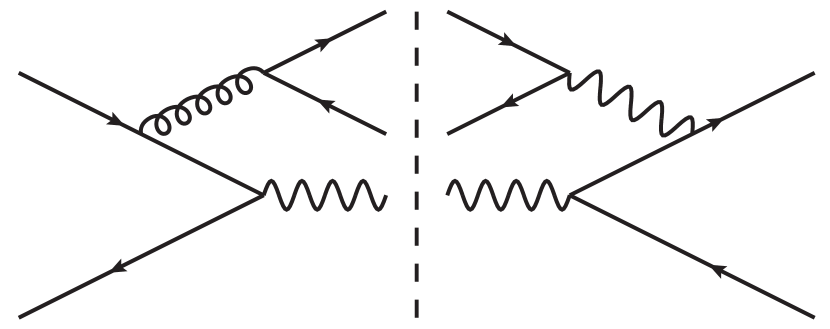
(a) (a)

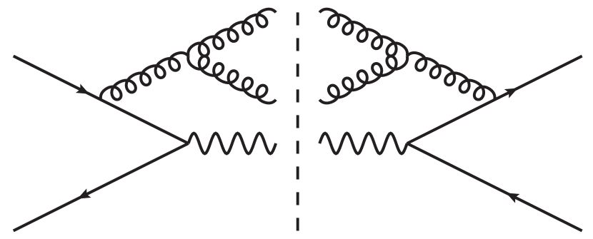
(b) (b)

                  

Figure 1: Contributions to the colour factors $C_{F}T_{R}$ (left) and $C_{A}C_{F}$ (right).

The case of the colour factor $C_{A}C_{F}$ is very similar. The colour factors $C_{A}$ originate either from diagrams with three-gluon vertices (see Fig. 1(b)) or from the non-commutative nature of generators of $SU(3)$ colour algebra in the fundamental representation. Neither of these issues apply to the case of mixed QCD$\otimes$QED corrections. The corresponding contributions can be eliminated by setting $C_{A}$ to zero in the NNLO QCD computation.

Finally, we need to understand how $C_{F}^{2}$ colour factors should be modified for the purpose of computing mixed QCD$\otimes$QED corrections. We consider a collision of a quark $q$ with an anti-quark $\bar{q}$, assume that the electric charge of the quark is $e_{q}$, and discuss a few illustrative examples.

Consider the double-virtual corrections, shown on the top line of Fig. 2. Upon setting $C_{A}$ to zero, colour traces that appear in both planar and non-planar diagrams provide a colour factor $C_{F}^{2}$. Since any of the two gluon lines can be replaced by a photon line in any of these diagrams, the required modification of the colour factor is $C_{F}^{2}\to 2C_{F}e_{q}^{2}$. It is easy to see that the same holds for real-virtual contributions, shown on the second line of Fig. 2, and for interferences that arise between double-real contributions (see the final line Fig. 2).

A distinct situation arises in cases when two gluons appear in the final state, shown in Fig. 3. In this case, two diagrams in the QCD case are mapped onto two diagrams in the QCD$\otimes$QED case; hence, it appears at first sight that for these diagrams the correct replacement rule is $C_{F}^{2}\to C_{F}e_{q}^{2}$, so that the factor of two is missing. However, this is not the case because contributions of diagrams with two gluons to the cross section are multiplied by a factor $1/2!$ to account for the symmetric final state. Clearly, there is no such factor in case of the $g+\gamma$ final state. This mismatch is accounted for if the colour factor $C_{F}^{2}$ in the $q\bar{q}\to Z+g+g$ contribution is again replaced by $2C_{F}e_{q}^{2}$, in accord with what is needed for double-virtual and real-virtual contributions.

Figure 2: Contributions to the colour factor $C_{F}^{2}$ and their abelianised counterparts.

Hence, after an examination of all the cases, we conclude that for processes with an incoming quark-antiquark pair or interference-like contributions with two identical quarks, we replace

$$C_{F}^{2}\rightarrow 2C_{F}e_{q}^{2}\ ,\;\;\;T_{R}\to 0\ ,\;\;\;\;C_{A}\to 0\ ,$$ (1)

in the formulas that describe NNLO QCD corrections to $Z$ boson production and obtain results for mixed QCD$\otimes$QED corrections. In Eq. (1), $e_{q}$ is the electric charge of the incoming quark.

$$\frac{1}{2}\left(\left|\leavevmode\hbox{$\vbox{\hbox{\resizebox{}{}{{\leavevmode\hbox{\set@color{\includegraphics[width=86.72267pt]{figures/as2_topo/rrgg1.eps}}}}}}}$}+\leavevmode\hbox{$\vbox{\hbox{\resizebox{}{}{{\leavevmode\hbox{\set@color{\includegraphics[width=86.72267pt]{figures/as2_topo/rrgg2.eps}}}}}}}$}\right|^{2}\right)\longrightarrow\left|\leavevmode\hbox{$\vbox{\hbox{\resizebox{}{}{{\leavevmode\hbox{\set@color{\includegraphics[width=65.04034pt]{figures/asa_topo/rrag.eps}}}}}}}$}\right|^{2}+\left|\leavevmode\hbox{$\vbox{\hbox{\resizebox{}{}{{\leavevmode\hbox{\set@color{\includegraphics[width=65.04034pt]{figures/asa_topo/rrga.eps}}}}}}}$}\right|^{2}$$

Figure 3: Contributions to the colour factor $C_{F}^{2}$ and their abelianised counterparts.

For processes with an incoming (anti)quark and a gluon, there is no symmetry factor, and the two possible ways to replace a gluon by a photon amount to the two distinct processes $qg\rightarrow Z+q+\gamma$ and $q\gamma\rightarrow Z+q+g$. The replacement rules become

$$C_{F}^{2}\rightarrow C_{F}e_{q}^{2}\ ,\;\;\;C_{A}\to 0\ .$$ (2)

Similarly, for processes induced by two gluons, replacing a gluon by a photon leads to the processes $g\gamma\rightarrow Z+q\bar{q}$ and $\gamma g\rightarrow Z+q\bar{q}$. We then have the replacement rule

$$C_{F}^{2}\rightarrow C_{F}e_{q}^{2}\ ,\;\;\;C_{A}\to 0\ .$$ (3)

We also note that, if photon-induced contributions are obtained from gluon-induced processes, the averaging over colour charges of the incoming partons has to be changed as well.

Making use of the procedure described above, we abelianised the fully-differential description of the on-shell $Z$ boson production given in Ref. Caola:2019nzf , including regulated double-real and real-virtual contributions, integrated subtraction terms and the virtual contributions. This gives us an opportunity to compute mixed QCD$\otimes$QED corrections to any infrared-safe observable in the production of an on-shell $Z$ boson.

2.3 Implementation of $Z$ boson decay

We now discuss the treatment of the decay of the $Z$ boson into massless leptons, $Z\to\ell^{+}\ell^{-}$, in QCD and QED perturbative expansions. At leading order, the cross section for the production of an on-shell $Z$ boson is computed from the tree-level process $q\bar{q}\rightarrow Z\rightarrow\ell^{+}\ell^{-}$, where the square of the propagator of an intermediate $Z$ boson is replaced by its narrow width limit

$$\frac{1}{(Q^{2}-M_{Z}^{2})^{2}+M_{Z}^{2}\Gamma_{Z}^{2}}\rightarrow\frac{\pi}{M_{Z}\Gamma_{Z}}\delta(Q^{2}-M_{Z}^{2})\ .$$ (4)

In Eq. (4) $Q$ is the four-momentum of the $Z$ boson and $\Gamma_{Z}$ is its width. In principle, the width of the $Z$ boson in Eq. (4) receives perturbative corrections. These corrections should, partially, cancel QED corrections to $Z\rightarrow\ell^{+}\ell^{-}$ that are included in our calculation. In order to account for that, we rewrite the cross section for $pp\rightarrow Z\rightarrow\ell^{+}\ell^{-}$ as follows

$$\mathop{}\!\mathrm{d}\sigma_{pp\rightarrow Z\rightarrow\ell^{+}\ell^{-}}=\frac{\mathop{}\!\mathrm{d}\sigma_{pp\rightarrow Z}\mathop{}\!\mathrm{d}\Gamma_{Z\rightarrow\ell^{+}\ell^{-}}}{\Gamma_{Z}}=\text{Br}_{Z\rightarrow\ell^{+}\ell^{-}}\times\mathop{}\!\mathrm{d}\sigma_{pp\rightarrow Z}\times\frac{\mathop{}\!\mathrm{d}\Gamma_{Z\rightarrow\ell^{+}\ell^{-}}}{\Gamma_{Z\rightarrow\ell^{+}\ell^{-}}}\ .$$ (5)

In Eq. (5) we introduced the branching ratio of the $Z$ boson decay to a massless $\ell^{+}\ell^{-}$ pair $\text{Br}_{Z\rightarrow\ell^{+}\ell^{-}}$; we will treat it as an experimental input parameter and will not expand it in $\alpha_{s}$ and $\alpha$. However, all other terms in Eq. (5) will be treated within QCD/QED perturbation theory. In particular, the ratio $\mathop{}\!\mathrm{d}\Gamma_{Z\rightarrow\ell^{+}\ell^{-}}/\Gamma_{Z\rightarrow\ell^{+}\ell^{-}}$ must be expanded to first order in $\alpha$. We write

$$\begin{split}\Gamma_{Z\rightarrow\ell^{+}\ell^{-}}=&\Gamma_{Z\rightarrow\ell^{+}\ell^{-}}^{(0)}+\Gamma_{Z\rightarrow\ell^{+}\ell^{-}}^{(1)}+{\cal O}(\alpha^{2})\ ,\\ \mathop{}\!\mathrm{d}\Gamma_{Z\rightarrow\ell^{+}\ell^{-}}=&\mathop{}\!\mathrm{d}\Gamma_{Z\rightarrow\ell^{+}\ell^{-}}^{(0)}+\mathop{}\!\mathrm{d}\Gamma_{Z\rightarrow\ell^{+}\ell^{-}}^{(1)}+{\cal O}(\alpha^{2})\ ,\end{split}$$ (6)

and expand the ratio

$$\frac{\mathop{}\!\mathrm{d}\Gamma_{Z\rightarrow\ell^{+}\ell^{-}}}{\Gamma_{Z\rightarrow\ell^{+}\ell^{-}}}=\frac{\mathop{}\!\mathrm{d}\Gamma_{Z\rightarrow\ell^{+}\ell^{-}}^{(0)}}{\Gamma_{Z\rightarrow\ell^{+}\ell^{-}}^{(0)}}+\left[-\frac{\mathop{}\!\mathrm{d}\Gamma_{Z\rightarrow\ell^{+}\ell^{-}}^{(0)}\Gamma_{Z\rightarrow\ell^{+}\ell^{-}}^{(1)}}{\left(\Gamma_{Z\rightarrow\ell^{+}\ell^{-}}^{(0)}\right)^{2}}+\frac{\mathop{}\!\mathrm{d}\Gamma_{Z\rightarrow\ell^{+}\ell^{-}}^{(1)}}{\Gamma_{Z\rightarrow\ell^{+}\ell^{-}}^{(0)}}\right]+\mathcal{O}(\alpha^{2})\ .$$ (7)

By construction, the above expression integrates to one over the unrestricted decay phase-space, so that terms in the square brackets integrate to zero. The expansion coefficients of the leptonic $Z$ width read

$$\Gamma_{Z\rightarrow\ell^{+}\ell^{-}}^{(0)} =\frac{G_{F}M_{Z}^{3}}{6\sqrt{2}\pi}\left(\frac{1}{4}+\left(\frac{1}{2}-2\sin^{2}\theta_{W}\right)^{2}\right)\ ,$$ (8)

$$\Gamma_{Z\rightarrow\ell^{+}\ell^{-}}^{(1)} =\Gamma_{Z\rightarrow e^{+}e^{-}}^{(0)}\times\frac{3\alpha}{4\pi}\ .\$$ (9)

We now go back to Eq. (5) and expand all relevant ingredients in series in the strong and electromagnetic coupling constants. To present the results of such an expansion, we denote the $\mathcal{O}(\alpha_{s}^{n}\;\alpha^{m})$ contribution to the $Z$ production cross section as $\sigma_{pp\rightarrow Z}^{(n,m)}$, and find the following results for $pp\to Z\to\ell^{+}\ell^{-}$ cross sections

$$\mathop{}\!\mathrm{d}\sigma_{\mathrm{LO}}^{\phantom{()}} =\text{Br}_{Z\rightarrow\ell^{+}\ell^{-}}\times\mathop{}\!\mathrm{d}\sigma^{(0,0)}_{pp\rightarrow Z}\times\frac{\mathop{}\!\mathrm{d}\Gamma^{(0)}}{\Gamma^{(0)}}\ ,$$ (10)

$$\mathop{}\!\mathrm{d}\sigma^{(\alpha_{s})}_{\mathrm{NLO}} =\text{Br}_{Z\rightarrow\ell^{+}\ell^{-}}\times\mathop{}\!\mathrm{d}\sigma^{(1,0)}_{pp\rightarrow Z}\times\frac{\mathop{}\!\mathrm{d}\Gamma^{(0)}}{\Gamma^{(0)}}\ ,$$ (11)

$$\mathop{}\!\mathrm{d}\sigma^{(\alpha)}_{\mathrm{NLO}} =\text{Br}_{Z\rightarrow\ell^{+}\ell^{-}}\times\left[\mathop{}\!\mathrm{d}\sigma^{(0,1)}_{pp\rightarrow Z}\times\frac{\mathop{}\!\mathrm{d}\Gamma^{(0)}}{\Gamma^{(0)}}+\mathop{}\!\mathrm{d}\sigma^{(0,0)}_{pp\rightarrow Z}\times\left(\frac{\mathop{}\!\mathrm{d}\Gamma^{(1)}}{\Gamma^{(0)}}-\frac{\mathop{}\!\mathrm{d}\Gamma^{(0)}}{\Gamma^{(0)}}\times\frac{3\alpha}{4\pi}\right)\right]\ ,$$ (12)

$$\mathop{}\!\mathrm{d}\sigma^{(\alpha_{s}^{2})}_{\mathrm{NNLO}} =\text{Br}_{Z\rightarrow\ell^{+}\ell^{-}}\times\mathop{}\!\mathrm{d}\sigma^{(2,0)}_{pp\rightarrow Z}\times\frac{\mathop{}\!\mathrm{d}\Gamma^{(0)}}{\Gamma^{(0)}}\ ,$$ (13)

$$\mathop{}\!\mathrm{d}\sigma^{(\alpha_{s}\alpha)}_{\mathrm{NNLO}} =\text{Br}_{Z\rightarrow\ell^{+}\ell^{-}}\times\left[\mathop{}\!\mathrm{d}\sigma^{(1,1)}_{pp\rightarrow Z}\times\frac{\mathop{}\!\mathrm{d}\Gamma^{(0)}}{\Gamma^{(0)}}+\mathop{}\!\mathrm{d}\sigma^{(1,0)}_{pp\rightarrow Z}\times\left(\frac{\mathop{}\!\mathrm{d}\Gamma^{(1)}}{\Gamma^{(0)}}-\frac{\mathop{}\!\mathrm{d}\Gamma^{(0)}}{\Gamma^{(0)}}\times\frac{3\alpha}{4\pi}\right)\right]\ .$$ (14)

Note that terms in round brackets in Eqs. (12) and (14) integrate to zero over an unrestricted phase-space, such that the inclusive cross section is given by a product of the branching fraction and the production cross section, as expected from Eq. (5). We emphasise again that we consider massless leptons throughout this paper.

To present our results for QCD$\otimes$QED corrections, we define ratios of contributions to the cross section at different perturbative orders. We write

$$\Delta_{\alpha}=\frac{\sigma^{(\alpha)}_{\mathrm{NLO}}}{\sigma_{\mathrm{LO}}^{\phantom{()}}+\sigma^{(\alpha_{s})}_{\mathrm{NLO}}}\ ,\;\;\;\;\;\;\Delta_{\alpha_{s}^{2}}=\frac{\sigma^{(\alpha_{s}^{2})}_{\mathrm{NNLO}}}{\sigma_{\mathrm{LO}}^{\phantom{()}}+\sigma^{(\alpha_{s})}_{\mathrm{NLO}}}\ ,\;\;\;\;\;\;\Delta_{\alpha_{s}\alpha}=\frac{\sigma^{(\alpha_{s}\alpha)}_{\mathrm{NNLO}}}{\sigma_{\mathrm{LO}}^{\phantom{()}}+\sigma^{(\alpha_{s})}_{\mathrm{NLO}}}\ .$$ (15)

To discuss kinematic distributions, we define differential bin-by-bin corrections in a similar fashion

$$\mathop{}\!\mathrm{d}\Delta_{\alpha}=\frac{{\rm d}\sigma^{(\alpha)}_{\mathrm{NLO}}}{{\rm d}\sigma_{\mathrm{LO}}^{\phantom{()}}+{\rm d}\sigma^{(\alpha_{s})}_{\mathrm{NLO}}}\ ,\;\;\mathop{}\!\mathrm{d}\Delta_{\alpha_{s}^{2}}=\frac{{\rm d}\sigma^{(\alpha_{s}^{2})}_{\mathrm{NNLO}}}{{\rm d}\sigma_{\mathrm{LO}}^{\phantom{()}}+{\rm d}\sigma^{(\alpha_{s})}_{\mathrm{NLO}}}\ ,\;\;\mathop{}\!\mathrm{d}\Delta_{\alpha_{s}\alpha}=\frac{{\rm d}\sigma^{(\alpha_{s}\alpha)}_{\mathrm{NNLO}}}{{\rm d}\sigma_{\mathrm{LO}}^{\phantom{()}}+{\rm d}\sigma^{(\alpha_{s})}_{\mathrm{NLO}}}\ .$$ (16)

2.4 Checks of the computation

Although the abelianisation procedure is, in principle, straightforward, its implementation in a fully-differential NNLO QCD computation is tedious. For this reason, it is important to check the implementation. We did this in the following way. In addition to abelianising the fully-differential NNLO QCD computation in Ref. Caola:2019nzf , we also abelianised the analytic NNLO QCD coefficients for inclusive Z boson production given in Ref. Hamberg:1990np and compared these to analytic expressions for mixed QCD$\otimes$QED corrections given in appendix B of Ref. deFlorian:2018wcj . We then used our abelianised analytic expressions to compute the inclusive on-shell production cross section of $pp\to Z$ and check that it agrees with the cross section obtained using the fully-differential implementation of mixed QCD$\otimes$QED corrections.

3 Results

In this section we discuss mixed QCD$\otimes$QED corrections to various observables in $pp\to Z\to\ell^{+}\ell^{-}$ and compare them to other corrections. We consider the LHC with 13 TeV center-of-mass collision energy. We use $M_{Z}=91.1876~{}\mathrm{GeV}$ for the mass of the $Z$ boson, and consider its decay to a single flavour of massless leptons with a branching ratio $\text{Br}_{Z\rightarrow\ell^{+}\ell^{-}}=0.033632$. We compute the couplings of the $Z$ boson to leptons and quarks using $G_{F}=1.16639\times 10^{-5}~{}\mathrm{GeV}^{-2}$, $M_{W}=80.398~{}\mathrm{GeV}$ and $\sin^{2}\theta_{W}=0.2226459$ as the input parameters. We use the NNPDF3.1luxQED set with five active flavours Bertone:2017bme as provided by the LHAPDF interface Buckley:2014ana , and take all quark to be massless. To compute the $\Delta$-corrections defined in the previous Section, we always use parton distributions at NNLO accuracy to calculate all the relevant contributions. We set the renormalisation and factorisation scales to $\mu_{R}=\mu_{F}=M_{Z}$. The strong coupling constant is taken to be $\alpha_{S}(M_{Z})=0.118$ which is compatible with values provided by the NNPDF set. We describe photon interactions with leptons and quarks by the fine structure constant evaluated at the renormalisation scale $\mu=M_{Z}$; numerically, it is equal to $\alpha=1/128$.

3.1 Inclusive cross sections

We use the above setup to compute the inclusive cross section of $Z$ boson production at various (NLO QED, NNLO QCD and mixed QCD$\otimes$QED) approximations. Using notations introduced in the previous section, we find

$$\Delta_{\alpha}=3.2\cdot 10^{-3}\ ,\qquad\Delta_{\alpha_{s}^{2}}=-6.4\cdot 10^{-3}\ ,\qquad\Delta_{\alpha_{s}\alpha}=2.9\cdot 10^{-4}\ .$$ (17)

We note that the $\Delta$ ratios in Eq. (17) receive contributions from corrections to the production only, since corrections to the decay of the $Z$ boson $Z\to\ell^{+}\ell^{-}$ cancel with corrections to the partial decay width $\Gamma_{Z\to\ell^{+}\ell^{-}}$, as explained in the previous Section.

It follows from Eq. (17) that the magnitude of mixed QCD$\otimes$QED corrections to the inclusive cross section $pp\to Z$ is consistent with expectations. Indeed, they are smaller than NLO QED (NNLO QCD) corrections by a factor ten (twenty), respectively. These suppression factors are in accord with our expectations, based on the relative magnitude of strong and electromagnetic coupling constants.

We note that our results for the corrections to the inclusive cross section are different from the results of Ref. deFlorian:2018wcj . In particular, this reference reported a smaller suppression of the mixed QCD$\otimes$QED corrections relative to the NNLO QCD one. The reason for this is that Ref. deFlorian:2018wcj employs a four-flavour scheme to compute both NNLO QCD and mixed QCD$\otimes$QED corrections. Since both NNLO QCD and mixed QCD$\otimes$QED corrections exhibit a strong sensitivity to input parameters, thanks to a very strong cancellation between (large) corrections to $q\bar{q}$ and $qg$ partonic channels at the LHC energies deFlorian:2018wcj , even small changes in the input can lead to significant changes in final results for corrections. We have confirmed that if we use the same input, we agree with the results of Ref. deFlorian:2018wcj .

Finally, we comment on the scale dependence of the total NNLO cross section that includes the $\Delta_{\alpha_{s}^{2}}$ and $\Delta_{\alpha_{s}\alpha}$ corrections. Although this dependence is small, ${\cal O}(0.5-0.7\%)$, it is entirely dominated by pure QCD effects and it is not possible to unambigously identify the impact of QCD$\otimes$QED corrections on it. For this reason, we decided to avoid presenting results for the scale dependence of the NNLO cross section. Instead, to understand the dependence of the QCD$\otimes$QED corrections on the scale choice, we consider the $\Delta_{\alpha_{s}\alpha}$ correction where the cancellation between the $\mu$-dependence of parton distribution functions and the explicit scale dependence of the NNLO contribution cannot be expected. Because of that, it is not surprising that these corrections appear to be rather sensitive to the choice of the factorisation and the renormalisation scales $\mu$. Indeed, by choosing the scale $\mu=\left[M_{Z}/2,M_{Z},2M_{Z}\right]$, we obtain the corrections $\Delta_{\alpha_{s}\alpha}=\left[5.6,2.9,-0.28\right]\cdot 10^{-4}$. Although a stronger sensitivity of the correction $\Delta_{\alpha_{s}\alpha}$ to the choice of the scale is expected, there is yet another reason for large variations in $\Delta_{\alpha_{s}\alpha}$. In fact, the enhanced dependence on $\mu$ can be also traced back to a strong cancellation between quark- and gluon-initiated contributions to $\Delta_{\alpha_{s}\alpha}$ which is affected by the change of the scale $\mu$ in a significant way.

As we discuss in the next Section, the cancellation between $q\bar{q}$ and $qg$ channels is also an important feature of mixed corrections to fiducial cross sections. We therefore expect that for the fiducial cases the scale variation of mixed corrections will exhibit similar behaviour. For this reason, we will not discuss the scale dependences of those corrections any further in the next section.

3.2 Fiducial cross sections

Fiducial cross sections are defined through kinematic selection criteria applied to physical objects in final states. We define the selection criteria for $pp\to Z\to\ell^{+}\ell^{-}$ as

$$p_{\perp,\ell_{1}}>24~{}\mathrm{GeV}\ ,\quad p_{\perp,\ell_{2}}>16~{}\mathrm{GeV}\ ,\quad|y_{\ell_{i}}|<2.4\ ,\;\;\;\;50~{}\mathrm{GeV}<m_{\ell\bar{\ell}}<120~{}{\rm GeV}\ ,$$ (18)

where $\ell_{1,2}$ denote leptons with leading and subleading transverse momenta, respectively.

Since we work with massless leptons, their transverse momenta are not collinear-safe observables; for this reason, we need to introduce an analog of QCD jets for leptons by combining leptons with collinear photons. Such recombination procedures are also used in experimental measurements to define “physical” electrons subject to selection cuts.

For the purposes of the computation of mixed QCD$\otimes$QED corrections, we choose a simplified version of the standard recipe Alioli:2016fum . To this end, we begin by computing two quantities $R_{\ell^{\pm}\gamma}=\sqrt{(y_{\ell^{\pm}}-y_{\gamma})^{2}+(\varphi_{\ell^{\pm}}-\varphi_{\gamma})^{2}}$ where $y_{\ell^{\pm},\gamma}$ are the rapidities and $\varphi_{\ell^{\pm},\gamma}$ the azimuthal angles of the lepton or antilepton, and the photon, respectively. If $R_{\ell^{\pm}\gamma}$ for the photon and one of the leptons is smaller than some $R_{\mathrm{min}}$, the photon is recombined with the lepton by adding their momenta; the new object is treated as a lepton inasmuch as the selection cuts Eq. (18) are concerned. In this paper, we use the standard value Alioli:2016fum $R_{\mathrm{min}}=0.1$.

As we already mentioned, there are three distinct sources of QED corrections. To show them separately, we decompose the NLO QED and mixed QCD$\otimes$QED results according to whether the QED correction is associated with the production of the $Z$ boson ($P$), its decay ($D$), or its decay width $\Gamma_{Z\to e^{+}e^{-}}$ ($W$). Using the definitions for $\Delta$’s in the previous Section, we find

$$\begin{split}&\Delta_{\alpha}=(3.0\cdot 10^{-3})_{P}-(7.2\cdot 10^{-3})_{D}-(1.6\cdot 10^{-3})_{W}\ ,\\ &\Delta_{\alpha_{s}^{2}}=-(1.2\cdot 10^{-2})\ ,\\ &\Delta_{\alpha_{s}\alpha}=-(1.5\cdot 10^{-4})_{P\otimes P}-(4.9\cdot 10^{-3})_{P\otimes D}-(0.3\cdot 10^{-3})_{P\otimes W}\ .\end{split}$$ (19)

The many results in Eq. (19) can be compared in different ways. First, we note that the QCD corrections are larger than in the inclusive case by almost a factor of two whereas the NLO QED corrections (initial) do not change significantly. The mixed QCD$\otimes$QED correction to the production is, on the other hand, smaller by a factor of two than in the inclusive case. Similar to the inclusive case, the relative magnitude of NLO QED, NNLO QCD and mixed QCD$\otimes$QED corrections to the fiducial $Z$ boson production cross section is consistent with expectations based on the relative sizes of QCD and QED couplings, despite the somewhat larger relative magnitude of the NNLO QCD correction.

It is interesting to understand how the final result for QCD$\otimes$QED corrections to the production comes about. To this end, it is instructive to decompose $[\Delta_{\alpha_{s}\alpha}]_{P\otimes P}$ into contributions of particular partonic channels, see Table 1. We observe a sizeable, almost an order-of-magnitude cancellation between $q\bar{q}$ and $qg$ channels. In fact a similar cancellation reduces the magnitude of NNLO QCD corrections which could have been quite a bit bigger than what they are if this cancellation was not present.

It is seen from Table 1 that contributions of photon-induced channels are very small, as expected. However, due to the aforementioned cancellation, they still contribute roughly twenty percent to the total result for mixed initial-initial corrections. It is also interesting that the photon-induced contributions are larger than those of $qq$ channels. This implies that neglecting contributions with photons in the initial state is not a good approximation if QCD$\otimes$QED precision is desired.

Partonic Channel	$[\Delta_{\alpha_{s}\alpha}]_{P\otimes P}\cdot 10^{4}$
$q\bar{q}$	5.60
$qq$	0.13
$qg+gq$	-7.01
$q\gamma+\gamma q$	-0.32
$\gamma g$	0.06
${\rm Total}$	-1.54

Table 1: Contributions of the different partonic channels to $[\Delta_{\alpha_{s}\alpha}]_{P\otimes P}$.

A rather different situation arises if we look at contributions to Eq. (19) that involve corrections to $Z$ boson decays. They are described by $[\Delta_{\alpha}]_{D}$ and by $[\Delta_{\alpha_{s}\alpha}]_{P\otimes D}$ for the QED and QCD$\otimes$QED corrections, respectively. Inspecting Eq. (19), we observe that both of these contributions are large and that $[\Delta_{\alpha_{s}\alpha}]_{P\otimes D}$ is smaller than $[\Delta_{\alpha}]_{D}$ by only thirty percent in spite of being suppressed by one power of $\alpha_{s}$. This implies that for fiducial cross sections QED radiation in the decay is very strongly affected by QCD radiation in the production.

This result illustrates that the selection criteria shown in Eq. (18) are strongly impacted by the non-vanishing transverse momentum of the $Z$ boson that in the case of a fixed-order computation is provided by the initial state QCD radiation. In addition, $R_{\min}=0.1$ is probably too small an isolation cone to allow a stable perturbative description of QED radiation off the outgoing leptons. To illustrate this remark, we point out that, with $R_{\rm min}=0.1$ and an additional selection cut $p_{\perp,\gamma}>5~{}{\rm GeV}$, the rate of the $Z$ boson decay to three QED jets becomes close to four percent and thus much larger than a naive expectation based on $\alpha/\pi\sim 2\times 10^{-3}$ suppression of events with additional radiation. It is clear that a quasi-collinear fragmentation of a lepton to a photon, allowed by the selection cuts, may strongly change the observable cross section by reducing the transverse momentum of the lepton. Furthermore, we also observe that by rejecting events with two leptons and a photon and keeping events with only Born-like kinematics, the size of $[\Delta_{\alpha_{s}\alpha}]_{P\otimes D}$ gets reduced relative to $[\Delta_{\alpha}]_{D}$.

3.3 Kinematic distributions

We continue with the discussion of the impact of QCD$\otimes$QED corrections on kinematic distributions for the production of two leptons via an on-shell $Z$ boson at the LHC. Below we show the respective distribution at NLO QCD accuracy in upper panels and the relative corrections $\Delta_{\alpha_{s}^{2}}$, $\left[\Delta_{\alpha_{s}\alpha}\right]_{P\otimes P}$ and $\left[\Delta_{\alpha_{s}\alpha}\right]_{P\otimes D}$ in lower panels. We use the selection criteria shown in Eq. (18) and $R_{\rm min}=0.1$ throughout this section.

We begin with the discussion of the transverse momentum distribution of the two leptons, $p_{\perp,\ell\ell}$, shown in the left panels of Fig. 4. It is seen from the plot that both $\Delta_{\alpha_{s}^{2}}$ and $[\Delta_{\alpha_{s}\alpha}]_{P\otimes P}$ corrections become flat and positive above $p_{\perp,\ell\ell}\sim 20~{}{\rm GeV}$. In that region, the NNLO QCD corrections amount to ${\cal O}(40)$ percent. Although this is quite a large correction, we note that in this kinematic region they can be considered as NLO QCD corrections to $Z+{\rm jet}$ production. The mixed $[\Delta_{\alpha_{s}\alpha}]_{P\otimes P}$ corrections can be thought of as QED corrections to the NLO QCD distribution; this would suggest a percent-level correction. In fact, initial-initial corrections in this case turn out to be even smaller, of the order of two permille for $p_{\mathrm{T,\ell\ell}}>20~{}$GeV. This is partially due to the cancellation between $q\bar{q}$- and $qg$-induced contributions that we already discussed. For smaller values of the $Z$ transverse momentum, the corrections become large and negative; however, resummation may be needed to obtain a reliable prediction in this region.

Figure 4: Relative differential corrections $\Delta$ for the transverse momentum (left) and rapidity (right) of the dilepton system, $p_{\perp,\ell\ell}$ and $y_{\ell\ell}$. See text for further details.

The initial-final correction $[\Delta_{\alpha_{s}\alpha}]_{P\otimes D}$ to the $p_{\perp,\ell\ell}$ distribution of a lepton pair shows quite a different behaviour, with a maximum at $p_{\perp,\ell\ell}\simeq 30~{}$GeV. This feature appears because of an interplay of a few contributions with different kinematics features. On the one hand, processes without initial-state QCD radiation but with final-state photon emission yield a pair of leptons with a total transverse momentum smaller than $M_{Z}/2$. Moreover, the selection cuts we use further restrict it to $p_{\perp,\ell\ell}\lesssim~{}31~{}$GeV. On the other hand, processes with initial state radiation boost the $Z$ boson, leading to a tail which extends beyond this kinematic limit. This behaviour can already be observed in the initial and final contributions at NLO QED accuracy.

It is also interesting to point out that, although initial-final $[\Delta_{\alpha_{s}\alpha}]_{P\otimes D}$ corrections are indeed larger than initial-initial corrections $[\Delta_{\alpha_{s}\alpha}]_{P\otimes P}$ for almost all values of the transverse momentum $p_{\perp,\ell\ell}$, it is not the case for $p_{\perp,\ell\ell}\sim~{}30~{}{\rm GeV}$ where the initial-final correction passes through zero(s). For those values of $p_{\perp,\ell\ell}$, the initial-final and initial-initial QCD$\otimes$QED contributions become comparable.

The rapidity distribution of the dilepton system at NLO QCD and the different corrections to it are displayed in the right panels of Fig. 4. The shape of the rapidity distribution is determined by the selection cuts which flatten the distribution for values $|y_{\ell\ell}|<1$. Inside this region, which represents the bulk of the cross section, the NNLO QCD correction is flat and negative and amounts to a decrease of the NLO QCD result by $\mathcal{O}(-2)$ percent. The NNLO QCD correction then crosses zero at rapidities $|y_{\ell\ell}|\simeq 1$ and increase to $\mathcal{O}(3)$ percent at large rapidities. The mixed $[\Delta_{\alpha_{s}\alpha}]_{P\otimes P}$ correction has a very similar shape; it decreases the NLO QCD distribution by $\mathcal{O}(-0.4)$ permille in the central region and increases it to $\mathcal{O}(+0.4)$ permille outside. In contrast to the previous two corrections, the initial-final $[\Delta_{\alpha_{s}\alpha}]_{P\otimes D}$ correction is negative for all rapidities and amounts to a decrease by about $\mathcal{O}(-7)$ permille in the central region. For rapidities $|y_{\ell\ell}|>1$, the initial-final correction becomes smaller but it remains a factor 5 larger than the initial-initial one. Hence, it follows that for the rapidity distribution of a lepton pair, the initial-final corrections always dominate over the initial-initial one.

Figure 5: Relative differential corrections $\Delta$ for the transverse momentum of the leading (left) and subleading (right) lepton, $p_{\perp,\ell_{1}}$ and $p_{\perp,\ell_{2}}$. See text for further details.

We show the transverse momentum distributions of the leading and the subleading leptons in Fig. 5. For the leading lepton, the NNLO QCD corrections enhance the distribution at large $p_{\perp,\ell_{1}}$, which is consistent with the additional boost that leptons get from the second initial-state emission. The feature at $p_{\perp,\ell_{1}}=M_{Z}/2$ is a Sudakov shoulder effect, which is known to appear close to kinematic boundaries. The NNLO QCD correction factor stabilises at ${\cal O}(40)$ percent for large values of $p_{\perp,\ell 1}$. The initial-initial correction $[\Delta_{\alpha_{s}\alpha}]_{P\otimes P}$ shows a similar behaviour at high $p_{\perp,\ell_{1}}$ where it is about two permille. Interestingly, the initial-initial correction also enhances the distribution at smaller values of the transverse momentum $p_{\perp,\ell_{1}}$. The initial-final correction $[\Delta_{\alpha_{s}\alpha}]_{P\otimes D}$ is negative at high and positive at small $p_{\perp,\ell_{1}}$; this is consistent with the picture of the final state leptons losing energy to QED radiation and decreasing their transverse momenta. The correction $[\Delta_{\alpha_{s}\alpha}]_{P\otimes D}$ changes from ${\cal O}(-3)$ percent for $p_{\perp,\ell_{1}}>M_{Z}/2$ to ${\cal O}(+3)$ percent for $p_{\perp,\ell_{1}}<M_{Z}/2$.

The transverse momentum distribution of the subleading lepton at NLO QCD accuracy has some features which impact the respective corrections. Indeed, in addition to the Sudakov shoulder at $p_{\perp,\ell_{2}}=M_{Z}/2$, the distribution also features a similar effect at $p_{\perp,\ell_{2}}=24~{}{\rm GeV}$, due to the fact that $24~{}{\rm GeV}$ is a cut on the minimal transverse momentum of the leading lepton. Since at leading order the transverse momenta of the two leptons must be equal to each other, the leading order $p_{\perp,\ell_{2}}$ distribution is truncated at this value also for the subleading lepton and the lower bins are only populated through higher order corrections.

In order to avoid displaying large fluctuations of radiative effects around the Sudakov shoulder at $p_{\perp,\ell_{2}}=M_{Z}/2$, we combined two bins between $40~{}{\rm GeV}$ and $48~{}$GeV into a single bin to present various corrections. Similar to the leading-lepton case, we observe large positive NNLO QCD and mixed $[\Delta_{\alpha_{s}\alpha}]_{P\otimes D}$ corrections for $p_{\perp,\ell_{2}}>M_{Z}/2$ that can be as large as $\mathcal{O}(50)$ percent for QCD and $\mathcal{O}(2)$ permille for mixed QCD$\otimes$QED. The initial-final correction $[\Delta_{\alpha_{s}\alpha}]_{P\otimes D}$ is negative and takes values between ${\cal O}(-2)$ and ${\cal O}(-4)$ percent.

Finally, we discuss distributions of $\cos\theta^{*}$, where $\theta^{*}$ is the angle between the three-momentum of one of the leptons and a unit vector constructed from the difference between three-momenta of the colliding protons in the rest frame of the dilepton system. Its cosine is given by the following formula Collins:1977iv

$$\cos\theta^{*}=\frac{P_{\ell^{-}}^{+}P_{\ell^{+}}^{-}-P_{\ell^{-}}^{-}P_{\ell^{+}}^{+}}{\sqrt{m^{2}_{\ell^{+}\ell^{-}}(m^{2}_{\ell^{+}\ell^{-}}+p_{\perp,\ell^{+}\ell^{-}})}}{}\frac{p_{z,\ell^{+}\ell^{-}}}{\left|p_{z,\ell^{+}\ell^{-}}\right|}\ ,$$ (20)

where $P_{i}^{\pm}=(E_{i}\pm p_{z,i})$. The $\cos\theta^{*}$-distribution is one of the few observables with strong sensitivity to the weak mixing angle $\sin^{2}\theta^{\ell}_{\rm eff}$; it is used in experimental analyses for this purpose Sirunyan:2018swq . The relevant input for this measurement is provided by $\cos\theta^{*}$ distributions for restricted $m_{\ell\ell}$ and $|y_{\ell\ell}|$ intervals.

To illustrate how various effects modify the $\cos\theta^{*}$ distributions, in Fig. 6 we show them for $0.6<|y_{\ell\ell}|<1.2$ and $1.8<|y_{\ell\ell}|<2.4$ rapidity intervals. The panels on the left describe the rapidity interval $0.6<|y_{\ell\ell}|<1.2$ and feature the distribution at NLO QCD accuracy with two well-separated maxima in the upper panel and NNLO QCD and mixed QCD$\otimes$QED corrections in the lower panel. The NNLO QCD corrections are below a percent level at small values of $\cos\theta^{*}$, but become large and negative at the boundaries of the distribution. The mixed $[\Delta_{\alpha_{s}\alpha}]_{P\otimes P}$ corrections are relatively flat and amount to roughly $0.3$ permille in the bulk of the distribution. They increase slightly at small values of $\cos\theta^{*}$, but become large and negative in the outermost non-vanishing bins. The initial-final $[\Delta_{\alpha_{s}\alpha}]_{P\otimes D}$ contribution is negative for all values of $\cos\theta^{*}$ and is relatively flat, taking values between one and two permille.

The $\cos\theta^{*}$ distribution for rapidities $1.8<|y_{\ell\ell}|<2.4$ is quite different. First, two maxima merge into one maximum located at small values of $\cos\theta^{*}$. For this reason, we only display results in the interval $-0.5<\cos\theta^{*}<0.5$. Second, all corrections in this case are rather flat. However, their magnitudes are comparable to those in the interval $0.6<|y_{\ell\ell}|<1.2$, with the NNLO QCD corrections being just few percent and the initial-initial correction $[\Delta_{\alpha_{s}\alpha}]_{P\otimes P}$ below a permille level. The initial-final $[\Delta_{\alpha_{s}\alpha}]_{P\otimes D}$ corrections are negative and are close to two permille.

Figure 6: Relative differential corrections $\Delta$ for the $\cos\theta^{*}$ distribution for $0.6<|y_{\ell\ell}|<1.2$ (left) and $1.8<|y_{\ell\ell}|<2.4$ (right). See text for further details.

4 Conclusion and outlook

In this article, we presented the calculation of mixed QCD$\otimes$QED corrections to the production of an on-shell $Z$ boson at the LHC. We made use of the nested soft-collinear subtraction scheme developed for NNLO QCD computations at a fully-differential level, and extended it to cover the mixed QCD$\otimes$QED corrections. We adopted the abelianisation procedure introduced in Ref. deFlorian:2018wcj and included partonic channels with photons in the initial state. Since we considered production of an on-shell $Z$ boson, interactions between initial state partons and decay products of the $Z$ boson can be neglected.

As an illustration of the fully-exclusive nature of our computation, we calculated the mixed QCD$\otimes$QED corrections to a number of observables such as the transverse momentum distributions of di-leptons and of the leading and subleading leptons, as well as the rapidity of the dilepton system and one of the Collins-Soper angles $\theta^{*}$. Initial-initial QCD$\otimes$QED corrections typically change these distributions at below a permille level whereas initial-final ones change them by a few permille. This is a factor hundred (ten) smaller than the effects of NNLO QCD corrections, respectively.

Finally, we note that the production of the on-shell $Z$ boson is a relatively simple case. In the future, it may be interesting to compute the mixed QCD$\otimes$QED corrections to the generic off-shell Drell-Yan process and to the production of an on-shell $W$ boson. Thanks to recent developments, both of these computations are now feasible. The case of $W$ production will require an extension of the nested soft-collinear subtraction scheme to the case of a charged resonance. This is an interesting problem that we plan to address in the future.

References

- (1) G. Aad et al. [ATLAS Collaboration], Phys. Lett. B 716 (2012) 1.
- (2) S. Chatrchyan et al. [CMS Collaboration], Phys. Lett. B 716 (2012) 30.
- (3) S. D. Drell and T. M. Yan, Phys. Rev. Lett. 25 (1970) 316 Erratum: [Phys. Rev. Lett. 25 (1970) 902].
- (4) M. L. Mangano, Adv. Ser. Direct. High Energy Phys. 26 (2016) 231.
- (5) M. Dittmar, F. Pauss and D. Zurcher, Phys. Rev. D 56 (1997) 7284.
- (6) V. A. Khoze, A. D. Martin, R. Orava and M. G. Ryskin, Eur. Phys. J. C 19 (2001) 313.
- (7) W. T. Giele and S. A. Keller, hep-ph/0104053.
- (8) S. Haywood et al., “Electroweak physics,” In *Geneva 1999, Standard model physics (and more) at the LHC* 117-230.
- (9) A. M. Sirunyan et al. [CMS Collaboration], Eur. Phys. J. C 78 (2018) no.9, 701.
- (10) R. D. Ball et al. [NNPDF Collaboration], Eur. Phys. J. C 77 (2017) no.10, 663.
- (11) L. A. Harland-Lang, A. D. Martin, P. Motylinski and R. S. Thorne, Eur. Phys. J. C 75 (2015) no.5, 204.
- (12) T. J. Hou et al., arXiv:1908.11394 [hep-ph].
- (13) S. Alekhin, J. Blümlein, S. O. Moch and R. Placakyte, PoS DIS 2016 (2016) 016.
- (14) M. Farina, G. Panico, D. Pappadopulo, J. T. Ruderman, R. Torre and A. Wulzer, Phys. Lett. B 772 (2017) 210.
- (15) G. Altarelli, R. K. Ellis and G. Martinelli, Nucl. Phys. B 157 (1979) 461.
- (16) R. Hamberg, W. L. van Neerven and T. Matsuura, Nucl. Phys. B 359, 343 (1991) Erratum: [Nucl. Phys. B 644, 403 (2002)].
- (17) W. L. van Neerven and E. B. Zijlstra, Nucl. Phys. B 382 (1992) 11 Erratum: [Nucl. Phys. B 680 (2004) 513].
- (18) R. V. Harlander and W. B. Kilgore, Phys. Rev. Lett. 88 (2002) 201801.
- (19) S. Catani, L. Cieri, G. Ferrera, D. de Florian and M. Grazzini, Phys. Rev. Lett. 103 (2009) 082001.
- (20) K. Melnikov and F. Petriello, Phys. Rev. Lett. 96 (2006) 231803.
- (21) K. Melnikov and F. Petriello, Phys. Rev. D 74 (2006) 114017.
- (22) R. Gavin, Y. Li, F. Petriello and S. Quackenbush, Comput. Phys. Commun. 182 (2011) 2388.
- (23) R. Gavin, Y. Li, F. Petriello and S. Quackenbush, Comput. Phys. Commun. 184 (2013) 208.
- (24) R. Boughezal, J. M. Campbell, R. K. Ellis, C. Focke, W. Giele, X. Liu, F. Petriello and C. Williams, Eur. Phys. J. C 77 (2017) no.1, 7.
- (25) T. Ahmed, M. Mahakhud, N. Rana and V. Ravindran, Phys. Rev. Lett. 113 (2014) no.11, 112002.
- (26) S. Catani, L. Cieri, D. de Florian, G. Ferrera and M. Grazzini, Nucl. Phys. B 888 (2014) 75.
- (27) U. Baur, O. Brein, W. Hollik, C. Schappacher and D. Wackeroth, Phys. Rev. D 65 (2002) 033007.
- (28) U. Baur, S. Keller and W. K. Sakumoto, Phys. Rev. D 57 (1998) 199.
- (29) B. Mistlberger, JHEP 1805 (2018) 028.
- (30) R. Bonciani, F. Buccioni, R. Mondini and A. Vicini, Eur. Phys. J. C 77 (2017) no.3, 187.
- (31) C. Anastasiou and K. Melnikov, Nucl. Phys. B 646 (2002) 220.
- (32) M. Heller, A. von Manteuffel and R. M. Schabinger, arXiv:1907.00491 [hep-th].
- (33) Y. Li and F. Petriello, Phys. Rev. D 86 (2012) 094034.
- (34) L. Barze, G. Montagna, P. Nason, O. Nicrosini, F. Piccinini and A. Vicini, Eur. Phys. J. C 73 (2013) no.6, 2474.
- (35) S. Dittmaier, A. Huss and C. Schwinn, Nucl. Phys. B 885 (2014) 318.
- (36) S. Dittmaier, A. Huss and C. Schwinn, Nucl. Phys. B 904 (2016) 216.
- (37) D. de Florian, M. Der and I. Fabre, Phys. Rev. D 98 (2018) no.9, 094008.
- (38) F. Caola, K. Melnikov and R. Röntsch, Eur. Phys. J. C 77 (2017) no.4, 248.
- (39) A. Manohar, P. Nason, G. P. Salam and G. Zanderighi, Phys. Rev. Lett. 117 (2016) no.24, 242002.
- (40) A. V. Manohar, P. Nason, G. P. Salam and G. Zanderighi, JHEP 1712 (2017) 046.
- (41) V. Bertone et al. [NNPDF Collaboration], SciPost Phys. 5 (2018) no.1, 008.
- (42) J. C. Collins and D. E. Soper, Phys. Rev. D 16 (1977) 2219.
- (43) F. Caola, K. Melnikov and R. Röntsch, Eur. Phys. J. C 79 (2019), 386.
- (44) S. Frixione, Z. Kunszt and A. Signer, Nucl. Phys. B 467 (1996) 399.
- (45) S. Frixione, Nucl. Phys. B 507 (1997) 295.
- (46) F. Caola, M. Delto, H. Frellesvig and K. Melnikov, Eur. Phys. J. C 78 (2018), no. 8, 687.
- (47) M. Delto and K. Melnikov, JHEP 1905 (2019) 148.
- (48) F. Caola, K. Melnikov and R. Röntsch, arXiv:1907.05398 [hep-ph].
- (49) A. Buckley, J. Ferrando, S. Lloyd, K. Nordström, B. Page, M. Rüfenacht, M. Schönherr and G. Watt, Eur. Phys. J. C 75 (2015) 132.
- (50) D. A. Dicus and S. S. D. Willenbrock, Phys. Rev. D 34 (1986) 148.
- (51) S. Alioli et al., Eur. Phys. J. C 77 (2017) no.5, 280.