Transversely trapping surfaces: Dynamical version

Abstract

We propose new concepts, a dynamically transversely trapping surface (DTTS) and a marginally DTTS, as indicators for a strong gravity region. A DTTS is defined as a two-dimensional closed surface on a spacelike hypersurface such that photons emitted from arbitrary points on it in transverse directions are acceleratedly contracted in time, and a marginally DTTS is reduced to the photon sphere in spherically symmetric cases. (Marginally) DTTSs have a close analogy with (marginally) trapped surfaces in many aspects. After preparing the method of solving for a marginally DTTS in the time-symmetric initial data and the momentarily stationary axisymmetric initial data, some examples of marginally DTTSs are numerically constructed for systems of two black holes in the Brill–Lindquist initial data and in the Majumdar–Papapetrou spacetimes. Furthermore, the area of a DTTS is proved to satisfy the Penrose-like inequality, $A_{0}\leq 4\pi(3GM)^{2}$, under some assumptions. Differences and connections between a DTTS and the other two concepts proposed by us previously, a loosely trapped surface [Prog. Theor. Exp. Phys. 2017, 033E01 (2017)] and a static/stationary transversely trapping surface [Prog. Theor. Exp. Phys. 2017, 063E01 (2017)], are also discussed. A (marginally) DTTS provides us with a theoretical tool to significantly advance our understanding of strong gravity fields. Also, since DTTSs are located outside the event horizon, they could possibly be related with future observations of strong gravity regions in dynamical evolutions.

E0, E31, A13

1 Introduction

There are two characteristic positions in a black hole spacetime. Taking a Schwarzschild spacetime as an example, one is the horizon $r=2GM$ that determines the black hole region, where $r$ is the circumferential radius, $G$ is the Newtonian constant of gravitation, and $M$ is the Arnowitt–Deser–Misner (ADM) mass that represents the total gravitational energy evaluated at spatial infinity. The region on and inside the horizon, $r\leq 2GM$, is not observable for distant observers. The other is the photon sphere $r=3GM$ on which circular orbits of photons exist. The photon sphere is related to various observable phenomena. For example, excitation of quasinormal modes of fields is closely related to the photon sphere Cardoso:2008 , and hence it affects the gravitational waveform from, e.g., the merger of two black holes (see Ref. Abbott:2016 for the first detection). Also, the edge of the black hole shadow in electromagnetic observations is determined by the photon sphere Virbhadra:1999 , or its extension, the fundamental photon orbits Cunha:2017 . Recently, the Event Horizon Telescope Collaboration has succeeded in observing the black hole shadow of a massive object at the center of the galaxy M87 EHTCollaboration:2019 .

There are various extended concepts of the horizon $r=2GM$, and the most famous ones are an event horizon and an apparent horizon. An event horizon is defined as the outer boundary of a black hole region from which nothing can escape to the outside region. Specifying the position of the event horizon is crucial to understanding the structure of a spacetime. An apparent horizon is a two-dimensional surface such that the expansion of outgoing null geodesics emitted from it vanishes. Assuming cosmic censorship, the singularity theorem tells us that the presence of an apparent horizon implies the existence of an event horizon outside, and thus restricts the global properties of the spacetime (see Chapt. 12.2 of Ref. Wald ). Extended concepts of $r=2GM$ like the event and apparent horizons, if properly defined, provide us with tools to greatly advance our understanding of the properties of spacetimes. This fact motivates us to consider extended concepts of the photon sphere $r=3GM$. In this paper, we study extended concepts of a photon sphere to characterize a strong gravity region outside a black hole.

One of the extended concepts of a photon sphere is a photon surface proposed in Ref. Claudel:2000 . A photon surface is defined as a timelike surface $S$ such that arbitrary photons emitted on arbitrary points on $S$ in arbitrary null tangent directions to $S$ continue to propagate on $S$. Unlike a photon sphere, a photon surface may change its shape and size in time. For example, a hyperboloid in a flat Minkowski spacetime becomes a photon surface Claudel:2000 . Therefore, the existence of a photon surface does not necessarily imply the presence of a strong gravity region. One may expect that a static photon surface in a static spacetime would become an indicator for the presence of a strong gravity region. However, the definition of a photon surface imposes such a strong condition on the behavior of photons that the spacetime must be highly symmetric in order to possess a static photon surface. Related to this, various uniqueness theorems have been studied for spacetimes with photon surfaces Cederbaum:2014 ; Cederbaum:2015a ; Yazadjiev:2015a ; Cederbaum:2015b ; Yazadjiev:2015b ; Yazadjiev:2015c ; Rogatko:2016 ; Yoshino:2016 ; Tomikawa:2016 ; Tomikawa:2017 . See also Refs. Gibbons:2016 ; Koga:2016 ; Shoom:2017 ; Koga:2018 ; Koga:2019a ; Koga:2019b for related discussions.

The present authors have also suggested two concepts to characterize a strong gravity region: A loosely trapped surface (LTS) Shiromizu:2017 and a transversely trapping surface (TTS) Yoshino:2017 (referred to as a static/stationary TTS in this paper). An LTS is defined from the behavior of the mean curvature $k$ in a flow of two-dimensional surfaces on a spacelike hypersurface $\Sigma$. A static/stationary TTS is defined as a static/stationary timelike surface $S$ in a static/stationary spacetime such that arbitrary photons emitted on arbitrary points on $S$ in arbitrary null tangent directions to $S$ propagate on $S$ or to the inside region of $S$. Then, inspired by the Penrose inequality Penrose:1973

$$A_{\rm AH}\leq 4\pi(2GM)^{2},$$ (1)

which is conjectured (and partly proved) to be satisfied by the area of an apparent horizon $A_{\rm AH}$, we have proved that the area $A_{0}$ of each of an LTS and the spatial section of a static/stationary TTS satisfies a Penrose-like inequality,

$$A_{0}\leq 4\pi(3GM)^{2},$$ (2)

under some assumptions (see also earlier work for a photon sphere in Ref. Hod:2017 ). The concept of a static/stationary TTS is used to classify surfaces in a Kerr spacetime Galtsov:2019a ; Galtsov:2019b . Shortcomings of our previous works are that in the case of an LTS, the relation to the behavior of photons cannot be read from the definition directly, and in the case of a static/stationary TTS, its straightforward generalization to dynamical cases does not necessarily represent a strong gravity region similarly to a photon surface. We consider that it is necessary to introduce a concept of a surface as a strong gravity indicator defined from the photon behavior, with applicability to dynamically evolving spacetimes.

Motivated by the above discussions, the purpose of this paper is threefold. First, we define a new concept, a dynamically transversely trapping surface (DTTS), that satisfies the above requirements. Roughly speaking, a DTTS is defined as a two-dimensional surface on a spacelike hypersurface such that photons emitted in transverse directions experience accelerated contraction due to strong gravity. A marginally DTTS is defined as a special case. The concept of a (marginally) DTTS has close analogy with a (marginally) trapped surface (or an apparent horizon). Note that the concept of a DTTS in this paper is different from that of a static/stationary TTS in Ref. Yoshino:2017 . This point will be discussed in detail.

Second, we show that a (marginally) DTTS is a well-defined concept, by explicitly constructing some examples numerically. We prepare the method of solving for marginally DTTSs in some restricted configurations, i.e. the time-symmetric initial data and the momentarily stationary axisymmetric initial data. Then, marginally DTTSs are numerically solved for in the systems of two equal-mass black holes in the Brill–Lindquist initial data Brill:1963 and the Majumdar–Papapetrou spacetime Majumdar:1947 ; Papapetrou:1947 .

Third, we clarify some of the general properties of DTTSs. To be specific, we prove that the area of a DTTS satisfies the Penrose-like inequality in Eq. (2) under some assumptions. We also prove that there are configurations where a DTTS is guaranteed to be an LTS at the same time.

This paper is organized as follows. In Sect. 2 we define the concepts of a DTTS, a dynamically transversely trapping region, and a marginally DTTS. In Sect. 3 we specify the configurations to be studied, i.e. the time-symmetric initial data and the momentarily stationary axisymmetric initial data, and useful formulas to calculate (marginally) DTTSs are presented. In Sect. 4, marginally DTTSs are explicitly constructed numerically for two-black-hole systems in the Brill–Lindquist initial data. In Sect. 5, marginally DTTSs are calculated for systems of two extremal black holes in the Majumdar–Papapetrou spacetimes. In Sect. 6 we prove that a DTTS satisfies the Penrose-like inequality in Eq. (2) under some assumptions, and we discuss the connection between DTTSs and LTSs in Sect. 7. Section 8 is devoted to a summary and discussions. In Appendices A and B, detailed derivations of the equations for marginally DTTSs in the Brill–Lindquist initial data and in the Majumdar–Papapetrou spacetimes are presented, respectively. Throughout the paper, we study in the framework of the theory of general relativity for four-dimensional spacetimes. We use the units in which the speed of light is unity, $c=1$, while the Newtonian constant of gravitation $G$ is explicitly shown.

2 Definition of dynamically transversely trapping surfaces

In this section we present the definition of a DTTS. In Sect. 2.1, we examine photon surfaces in a Schwarzschild spacetime in order to learn a lesson that motivates the definition of a DTTS. Then, a DTTS is defined in Sect. 2.2, and its meaning is discussed in Sect. 2.3. In Sect. 2.4, analogies between DTTSs and trapped surfaces are discussed.

2.1 Motivation from the Schwarzschild spacetime

Let us begin our discussion by examining photon surfaces in a Schwarzschild spacetime. Since a photon surface is composed of null geodesics, we study null geodesic equations below. The metric of a Schwarzschild spacetime is

$$ds^{2}=-f(r)dt^{2}+\frac{dr^{2}}{f(r)}+r^{2}(d\theta^{2}+\sin^{2}\theta d\phi^{2}),$$ (3)

with

$$f(r):=1-\frac{2GM}{r}.$$ (4)

From the $t$ and $\phi$ components of null geodesic equations on the equatorial plane $\theta=\pi/2$, we obtain the conservation laws of energy and angular momentum,

$$f(r)\dot{t} = E,$$ (5)

$$r^{2}\dot{\phi} = Eb,$$ (6)

where dot denotes the derivative with the affine parameter $\lambda$ of the null geodesic, and $E$ and $b$ are the energy and the impact parameter, respectively. The null condition leads to

$$f(r)\dot{t}^{2}=\frac{\dot{r}^{2}}{f(r)}+r^{2}\dot{\phi}^{2}.$$ (7)

From these equations, we have

$$\frac{dr}{dt}=\pm f(r)\sqrt{1-\frac{b^{2}}{r^{2}}f(r)}.$$ (8)

Solutions of the radial coordinate for the geodesic equations are obtained by integrating this equation. If $b>3\sqrt{3}\ GM$, the geodesic is confined in the region $r>3GM$ or $r<3GM$, and possesses a pericenter or an apocenter, respectively. If $b<3\sqrt{3}\ GM$, the geodesic does not have a turning point and crosses the photon sphere $r=3GM$ from the inside region (resp. outside region) to the outside region (resp. inside region) according to the plus (resp. minus) sign in Eq. (8) (see Ref. Gralla:2019 for a recent study on black hole shadows that has close connection to such behavior of photons). For a later convenience, we present the radial geodesic equations,

$$\ddot{r}=\frac{f^{\prime}}{2f}\dot{r}^{2}-\frac{ff^{\prime}}{2}\dot{t}^{2}+fr\dot{\phi}^{2}=\frac{E^{2}b^{2}}{r^{3}}\left(1-\frac{3GM}{r}\right),$$ (9)

where prime indicates derivative with respect to $r$ and the second equality is derived using Eqs. (5)–(7).

If a solution $r(t)$ to Eq. (8) is obtained, we can construct a photon surface Claudel:2000 by virtue of the spherical symmetry. At $t=0$, we consider photons with the same values of the radial position $r$ and the radial velocity $dr/dt$ but with arbitrary angular positions and arbitrary angular velocities. Since all such photons have the same radial dependence $r(t)$, they form a photon surface $S$. Since $r(t)$ can be arbitrarily large, the photon surface itself does not necessarily imply the existence of a strong gravity region. Therefore, we must find a quantity that is suitable as an indicator for a strong gravity region.

The induced geometry of $S$ is given by

$$ds^{2}=-\alpha^{2}dt^{2}+r^{2}(d\theta^{2}+\sin^{2}\theta d\phi^{2}),$$ (10)

with the lapse function

$$\alpha=\frac{b}{r}f(r).$$ (11)

We denote $t=\mathrm{const.}$ surfaces in $S$ by $\sigma_{t}$, and its induced metric and extrinsic curvature by $h_{ab}$ and $\bar{k}_{ab}:=(1/2){}^{(3)}\bar{\pounds}_{\bar{n}}h_{ab}$, respectively, where ${}^{(3)}\bar{\pounds}$ and $\bar{n}^{a}$ denote the Lie derivative in $S$ and the future-directed unit normal to $\sigma_{t}$ in $S$. The trace of the extrinsic curvature is

$$\bar{k}=\frac{2}{bf(r)}\frac{dr}{dt}.$$ (12)

Using Eq. (9), the Lie derivative of $\bar{k}$ with respect to $\bar{n}^{a}$ is calculated as

$${}^{(3)}\bar{\pounds}_{\bar{n}}\bar{k}=\frac{2}{r^{2}}\left(1-\frac{3GM}{r}\right).$$ (13)

Then, we find that if $\sigma_{t}$ is located outside (resp. inside) the photon sphere $r=3GM$, the value of ${}^{(3)}\bar{\pounds}_{\bar{n}}\bar{k}$ is positive (resp. negative). Physically, a photon surface is in accelerated expansion or decelerated contraction in the region $r>3GM$, and in decelerated expansion or accelerated contraction in the region $r<3GM$, reflecting the strength of gravity. Therefore, ${}^{(3)}\bar{\pounds}_{\bar{n}}\bar{k}$ is a good indicator for a strong gravity region, and this result motivates us to define a DTTS using the quantity ${}^{(3)}\bar{\pounds}_{\bar{n}}\bar{k}$.

2.2 Definition

Figure 1: Configuration to be considered. We consider a two-dimensional closed surface $\sigma_{0}$ in a spacelike hypersurface $\Sigma$ of a spacetime $\mathcal{M}$. A timelike hypersurface $S$ intersects with $\Sigma$ precisely at $\sigma_{0}$. Notations are also indicated. See text for details.

Before introducing the definition of a DTTS, it is appropriate to show the configuration to be considered and specify notations. Figure 1 presents the typical configuration to be studied. We consider a spacetime $\mathcal{M}$ with the metric $g_{ab}$, and $\nabla_{a}$ is the covariant derivative associated with $g_{ab}$. In $\mathcal{M}$, take a spacelike hypersurface $\Sigma$ whose future-directed timelike unit normal is $n^{a}$. A spatial metric $q_{ab}$ is induced on $\Sigma$ as

$$q_{ab}=g_{ab}+n_{a}n_{b},$$ (14)

and the extrinsic curvature is defined as

$$K_{ab}=\frac{1}{2}\pounds_{n}q_{ab},$$ (15)

where $\pounds$ is a Lie derivative with respect to $\mathcal{M}$. The derivative operator associated with $q_{ab}$ is denoted by $D_{a}$. In $\Sigma$, we take a two-dimensional closed orientable surface $\sigma_{0}$ in order to examine whether it is a DTTS or not. The induced metric of $\sigma_{0}$ is

$$h_{ab}=q_{ab}-\hat{r}_{a}\hat{r}_{b},$$ (16)

where $\hat{r}^{a}$ is the spacelike unit normal to $\sigma_{0}$ in $\Sigma$ (namely, $\hat{r}^{a}$ is tangential to $\Sigma$). The extrinsic curvature of $\sigma_{0}$ as a hypersurface in $\Sigma$ is introduced as

$$k_{ab}=\frac{1}{2}{}^{(3)}\pounds_{\hat{r}}h_{ab},$$ (17)

where ${}^{(3)}\pounds$ is a Lie derivative with respect to $\Sigma$. The covariant derivative associated with $h_{ab}$ is denoted by $\mathcal{D}_{a}$.

We introduce a timelike hypersurface $S$ in $\mathcal{M}$, which intersects with $\Sigma$ precisely at $\sigma_{0}$. Note that the two hypersurfaces $S$ and $\Sigma$ are not necessarily orthogonal to each other at $\sigma_{0}$, and therefore, the outward spacelike unit normal $\bar{r}^{a}$ to $S$ does not agree with $\hat{r}^{a}$ in general. The metric induced on $S$ is

$$\bar{p}_{ab}=g_{ab}-\bar{r}_{a}\bar{r}_{b},$$ (18)

and the extrinsic curvature of $S$ is defined by

$$\bar{K}_{ab}=\frac{1}{2}\pounds_{\bar{r}}\bar{p}_{ab}.$$ (19)

The covariant derivative associated with $\bar{p}_{ab}$ is denoted by $\bar{D}_{a}$. The two-dimensional surface $\sigma_{0}$ can be regarded as a hypersurface in $S$, and the future directed unit normal to $\sigma_{0}$ in this sense is denoted by $\bar{n}^{a}$. Note that $\bar{n}^{a}$ and $n^{a}$ are different from each other in general. The extrinsic curvature of $\sigma_{0}$ as a hypersurface in $S$ is defined by

$$\bar{k}_{ab}=\frac{1}{2}{}^{(3)}\bar{\pounds}_{\bar{n}}h_{ab},$$ (20)

where ${}^{(3)}\bar{\pounds}_{\bar{n}}$ is a Lie derivative associated with $S$.

We now introduce the definition of a DTTS. From the above example of the Schwarzschild spacetime, we consider the following definition to be the most appropriate definition of a DTTS:

Definition 1.

Suppose $\Sigma$ to be a smooth spacelike hypersurface of a spacetime $\mathcal{M}$. A closed orientable two-dimensional surface $\sigma_{0}$ in $\Sigma$ is a dynamically transversely trapping surface (DTTS) if and only if there exists a timelike hypersurface $S$ in $\mathcal{M}$ that intersects $\Sigma$ precisely at $\sigma_{0}$ and satisfies the following three conditions at arbitrary points on $\sigma_{0}$:

$$\bar{k}=0,$$ (the momentarily non-expanding condition); (21)

$$\mathrm{max}\left(\bar{K}_{ab}k^{a}k^{b}\right)=0,$$ (the marginally transversely trapping condition); (22)

$${}^{(3)}\bar{\pounds}_{\bar{n}}\bar{k}\leq 0,$$ (the accelerated contraction condition), (23)

where $k^{a}$ are arbitrary future-directed null vectors tangent to $S$ and the quantity $\pounds_{\bar{n}}\bar{k}$ is evaluated with a time coordinate in $S$ whose lapse function is constant on $\sigma_{0}$.

Due to the inequality in the condition in Eq. (23), if there is a DTTS in $\Sigma$, there are infinitely many DTTSs in $\Sigma$ in general. Using the concept of DTTSs, we introduce a dynamically transversely trapping region and a marginally DTTS by the following definitions:

Definition 2.

Consider a collection of DTTSs such that any two of these can be transformed to each other by continuous deformation keeping to DTTSs. The region in which these DTTSs exist is said to be a dynamically transversely trapping region (or, more generally, one of dynamically transversely trapping regions). If the outer boundary of a dynamically transversely trapping region satisfies

$${}^{(3)}\bar{\pounds}_{\bar{n}}\bar{k}=0,$$ (24)

it is said to be a marginally DTTS.

Readers may wonder why we explicitly require Eq. (24) for a marginally DTTS, since Eq. (24) is naturally expected to be satisfied by the fact that a marginally DTTS is a boundary of a dynamically transversely trapping region. This is because at least for now, we cannot deny the possibility that the outer boundary is given by an envelope of infinitely many DTTSs, and thus it is not a DTTS. Of course, it is quite uncertain whether such a case happens, and clarifying this point is interesting although it is beyond the scope of this paper. Note also that although Eq. (24) gives an equation for marginally DTTSs, not all of the solutions are marginally DTTSs, because some of them may be inner boundaries of dynamically transversely trapping regions, or may be immersed in those regions.

2.3 Description of the three conditions

Among the three conditions in Eqs. (21)–(23), the first two, the momentarily non-expanding condition of Eq. (21) and the marginally transversely trapping condition of Eq. (22), determine the behavior of $S$ in the neighborhood of $\sigma_{0}$. The third condition, Eq. (23), is to judge whether $\sigma_{0}$ exists in a strong gravity region. We discuss the meanings of the three conditions in more detail, one by one.

2.3.1 The momentarily non-expanding condition

There are infinitely many timelike hypersurfaces $S$ that intersect $\Sigma$ at $\sigma_{0}$, and the value of ${}^{(3)}\bar{\pounds}_{\bar{n}}\bar{k}$ strongly depends on the choice of $S$. For this reason, one must specify how to choose $S$, and the momentarily non-expanding condition is introduced in order to fix the behavior of $S$ up to the first order in time. The first-order behavior of $S$ is specified by the timelike tangent vectors $\bar{n}^{a}$ of $S$ at points on $\sigma_{0}$, and once $\bar{n}^{a}$ is chosen, the value of $\bar{k}$ is also determined because $\bar{k}_{ab}$ is a quantity that represents the first-order behavior of $h_{ab}$ in time as understood from Eq. (20). Conversely, requiring $\bar{k}=0$ (basically) determines the choice of $\bar{n}^{a}$, and thus the first-order behavior of $S$. To be specific, the tangent vector $\bar{n}^{a}$ can be given in terms of $n^{a}$ and $\hat{r}^{a}$ through the transformation,

$$\bar{n}^{a}=\frac{1}{\sqrt{1-\beta^{2}}}\left(n^{a}-\beta\hat{r}^{a}\right),$$ (25)

where $\beta=\beta(x^{i})$ is a function of the coordinates $x^{i}$ on $\sigma_{0}$. The condition $\bar{k}=0$ is then becomes an equation for $\beta(x^{i})$, and an appropriate $\bar{n}^{a}$ is obtained by solving this equation. Note that there are exceptional cases where $S$ is not uniquely specified by this procedure. For example, if we adopt time-symmetric initial data as $\Sigma$ and a minimal surface in $\Sigma$ as $\sigma_{0}$, the value of $\bar{k}$ vanishes for arbitrary $\beta(x^{i})$. In such cases, all surfaces $S$ with $\bar{k}=0$ must be taken into account.

The geometrical meaning of the momentarily non-expanding condition is as follows. Let us span Gaussian normal coordinates $(t,x^{i})$ in $S$ from $\sigma_{0}$, and denote the slice $t=\mathrm{const.}$ as $\sigma_{t}$. Here, $t$ is the time coordinate and $x^{i}$ are the coordinates to specify positions of points on each of $\sigma_{t}$. The momentarily non-expanding condition $\bar{k}=0$ means that each area element of $\sigma_{t}$ is unchanged up to the first order in time. Therefore, the area of $\sigma_{0}$ is locally extremal in a sequence of $\sigma_{t}$, and if the accelerated contraction condition of Eq. (23) is satisfied simultaneously, it is locally maximal.

2.3.2 The marginally transversely trapping condition

The marginally transversely trapping condition is introduced to determine the second-order behavior of $S$ in time using propagation of photons.

Consider a photon that is emitted from a point on $\sigma_{0}$ tangentially to $S$. The quantity $\bar{K}_{ab}k^{a}k^{b}$ in Eq. (22) represents whether the photon propagates in the inward direction of $S$ or not. In order to see this, let us consider a “virtual photon” confined in the hypersurface $S$ whose equation is given by $k^{a}\bar{D}_{a}k^{b}=0$. Rewriting with the four-dimensional quantities, we have

$$a^{c}=-(\bar{K}_{ab}k^{a}k^{b})\hat{r}^{c},$$ (26)

where $a^{c}=k^{d}\nabla_{d}k^{c}$ is the four-acceleration. From this equation, we understand that a real photon whose equation is given by $k^{a}\nabla_{a}k^{b}=0$ propagates into the inward (resp. outward) region of $S$ if $\bar{K}_{ab}k^{a}k^{b}$ is negative (resp. positive). If $\bar{K}_{ab}k^{a}k^{b}=0$, the photon travels on $S$ up to second order in time. The condition $\bar{K}_{ab}k^{a}k^{b}=0$ is required for a photon surface Claudel:2000 , while the condition $\bar{K}_{ab}k^{a}k^{b}\leq 0$ is required for a static/stationary TTS Yoshino:2017 .

The meaning of the marginally transversely trapping condition in Eq. (22) is as follows: $S$ must be chosen so that all photons emitted from points on $\sigma_{0}$ in arbitrary tangential directions to $S$ must propagate into the inside region of $S$ or precisely on $S$, and furthermore, at least one photon must propagate on $S$ (up to the second order in time). In other words, if we consider a collection of all such photons, they distribute in a region with a small thickness in general after they are emitted. Then, $S$ is adopted as the outer boundary of such a region.

2.3.3 The accelerated contraction condition

Once the surface $S$ is specified by the above two conditions, it is possible to calculate ${}^{(3)}\bar{\pounds}_{\bar{n}}\bar{k}$. This is a quantity determined by the second-order behavior of $S$ in time. Here, we have to remark that this is a coordinate-dependent quantity. The trace of the Ricci equation of $\sigma_{0}$ as a hypersurface in $S$ is

$${}^{(3)}\bar{\pounds}_{\bar{n}}\bar{k}=-{}^{(3)}\bar{R}_{ab}\bar{n}^{a}\bar{n}^{b}-\bar{k}_{ab}\bar{k}^{ab}+\frac{1}{\alpha}\mathcal{D}^{2}\alpha,$$ (27)

where ${}^{(3)}\bar{R}_{ab}$ is the Ricci tensor calculated by the metric $\bar{p}_{ab}$ induced on $S$, $\mathcal{D}^{2}:=\mathcal{D}_{a}\mathcal{D}^{a}$ is the Laplace operator on $\sigma_{0}$, and $\alpha$ is the lapse function of the time coordinate. Hence, ${}^{(3)}\bar{\pounds}_{\bar{n}}\bar{k}$ obviously depends on $\alpha$, and thus we have to specify how to choose $\alpha$. As remarked at the end of Definition 1, we require $\alpha=\mathrm{const.}$ on $\sigma_{0}$. Then, the last term of Eq. (27) vanishes and ${}^{(3)}\bar{\pounds}_{\bar{n}}\bar{k}$ is given only in terms of geometrical quantities.

Note that, due to the constancy of $\alpha$, the concept of a DTTS becomes different from that of a static/stationary TTS. In the case of a static/stationary TTS, we consider a static/stationary surface $S$ which is generated by the Lie drag of $\sigma_{0}$ along the integral lines of the timelike Killing vector field $\xi^{a}$ in a static/stationary spacetime $\mathcal{M}$ Yoshino:2017 . Then, the momentarily non-expanding condition of Eq. (21) is trivially satisfied. If we choose $\sigma_{0}$ that satisfies the marginally transversely trapping condition of Eq. (22), $S$ becomes a static/stationary TTS. However, in this situation, although $S$ satisfies ${}^{(3)}\bar{\pounds}_{\bar{n}}\bar{k}=0$ for the time coordinate associated with the timelike Killing vector field (i.e. for the choice $\alpha=\sqrt{-\xi_{a}\xi^{a}}$), ${}^{(3)}\bar{\pounds}_{\bar{n}}\bar{k}$ violates the accelerated contraction condition of Eq. (23) in general for the choice $\alpha=\mathrm{const.}$, except for spherically symmetric spacetimes. Hence, there exist cases that a static/stationary TTS is not a DTTS at the same time. Furthermore, as we will see in Sect. 5, there are also converse cases that a DTTS in a static spacetime is not a static TTS. For this reason, an inclusion relationship cannot be found between DTTSs and static/stationary TTSs.

2.4 Comparison with trapped surfaces

A DTTS (Definition 1) and a marginally DTTS (Definition 2) are defined so that they have similarity to a trapped surface and a marginally trapped surface, respectively.

A trapped surface $\sigma_{\rm TS}$ is a two-dimensional closed orientable surface in a spacelike hypersurface $\Sigma$ such that both the outgoing and ingoing null geodesic congruences have negative expansion, i.e. $\theta_{+}<0$ and $\theta_{-}<0$, respectively. A collection of trapped surfaces forms a trapped region, and the outer boundary of the trapped region is defined as a marginally trapped surface. On the marginally trapped surface, $\theta_{-}\leq 0$ and $\theta_{+}=0$ hold. A marginally trapped surface may have multiple connected components (among them, the outermost components are defined as the apparent horizons), and the location of each component is uniquely determined. Similarly, a DTTS is defined in a spacelike hypersurface $\Sigma$ and a collection of DTTSs forms a dynamically transversely trapping region. A marginally DTTS is defined in a similar manner as a marginally trapped surface, and the location of each marginally DTTS is uniquely determined.

A (marginally) trapped surface and a (marginally) DTTS have similar features of gauge invariance and gauge dependence. On one hand, a (marginally) trapped surface $\sigma_{\rm TS}$ (seen as a two-dimensional spacelike surface in $\mathcal{M}$) is a gauge-invariant concept in the sense that values of the two kinds of expansion, $\theta_{+}$ and $\theta_{-}$, do not depend on the choice of coordinates to calculate them. Suppose $\sigma_{\rm TS}$ is obtained as a (marginally) trapped surface in some spacelike hypersurface $\Sigma$. Then, if (marginally) trapped surfaces are surveyed on another spacelike hypersurface $\Sigma^{\prime}$ which intersects with $\Sigma$ precisely at $\sigma_{\rm TS}$, we would obtain $\sigma_{\rm TS}$ as a (marginally) trapped surface as well. Similarly, if a surface $\sigma_{0}$ is an intersection of two spacelike hypersurfaces $\Sigma$ and $\Sigma^{\prime}$, we would obtain the same conclusion concerning whether $\sigma_{0}$ is a (marginally) DTTS or not on both of the hypersurfaces, because the same timelike hypersurface $S$ should be constructed by virtue of the momentarily non-expanding condition of Eq. (21) and the marginally transversely trapping condition of Eq. (22). On the other hand, a marginally trapped surface has gauge-dependent feature in the sense that if we consider time evolution of a marginally trapped surface, its three-dimensional worldsheet, which is called the trapping horizon Hayward:1993 , depends on the choice of the time coordinate. Similarly, the worldsheet of a marginally DTTS should be dependent on the selected time coordinate as well.

Further similarity between a (marginally) trapped surface and a (marginally) DTTS can be found for their area, i.e. the Penrose inequality of Eq. (1) and the Penrose-like inequality of Eq. (2). This issue will be discussed in Sect. 6.

3 Configurations and useful formulas

In this paper, we solve for marginally DTTSs and discuss their properties in fairly restricted situations. Namely, we consider the situation where the timelike hypersurface $S$ that satisfies the momentarily non-expanding condition in Eq. (21) orthogonally intersects with the spacelike hypersurface $\Sigma$. In other words, we restrict our attention to the case where

$$\hat{r}^{a}=\bar{r}^{a}\qquad\textrm{and}\qquad n^{a}=\bar{n}^{a}$$ (28)

are satisfied. To be specific, we consider time-symmetric initial data and momentarily stationary axisymmetric initial data. First, we derive useful formulas that are applicable to these setups in Sect. 3.1, and then the two kinds of initial data are described in Sect. 3.2. Preparing the method of solving for (marginally) DTTSs in the case that $S$ is not orthogonal to $\Sigma$ is definitely necessary, and we plan to study this issue in a forthcoming paper.

3.1 Useful formulas

Let us span the coordinates $(t,r,x^{i})$ such that the timelike hypersurface $S$ is given by $r=0$ in the neighborhood of $\sigma_{0}$. Let $\alpha$ denote the time lapse function, and for simplicity, we assume the shift vector to be zero, $\beta^{a}:=t^{a}-\alpha n^{a}=0$, where $t^{a}$ is the basis of the coordinate $t$. The metric is given by

$$ds^{2}=-\alpha^{2}dt^{2}+\varphi^{2}dr^{2}+h_{ij}dx^{i}dx^{j}+2\gamma_{ri}drdx^{i},$$ (29)

where $\varphi$ is the lapse function of the radial coordinate $r$.

3.1.1 Formulas related to the marginally transversely trapping condition

First, we derive useful formulas to study the marginally transversely trapping condition of Eq. (22). Rewriting Eq. (17) for $k_{ab}$ in terms of four-dimensional quantities, we have

$$k_{ab}=\frac{1}{2}\pounds_{\hat{r}}h_{ab}+v_{a}n_{b}+v_{b}n_{a},$$ (30)

with

$$v_{a}=\frac{1}{2}h_{ab}\pounds_{n}\hat{r}^{b}.$$ (31)

By substituting $\bar{p}_{ab}$ given by Eq. (18) into the formula for $\bar{K}_{ab}$, Eq. (19), we obtain

$$\bar{K}_{ab}=-n_{a}n_{b}\frac{{}^{(3)}\pounds_{\hat{r}}\alpha}{\alpha}+\frac{1}{2}\pounds_{\hat{r}}h_{ab}$$ (32)

after some algebra. Therefore, we obtain the following decomposition of $\bar{K}_{ab}$ into time and space directions:

$$\bar{K}_{ab}=-n_{a}n_{b}\frac{{}^{(3)}\pounds_{\hat{r}}\alpha}{\alpha}+k_{ab}-v_{a}n_{b}-v_{b}n_{a}.$$ (33)

There are several other expressions for $v_{a}$, for example,

$$v_{a}=h_{ab}n^{c}\nabla_{c}\hat{r}^{b},$$ (34)

which is derived by expressing the right-hand side with $\bar{K}_{d}^{~{}b}=\bar{p}_{d}^{~{}c}\nabla_{c}\hat{r}^{b}$ and substituting Eq. (33). From Eqs. (31) and (34), we have

$$v_{a}=-h_{ab}\hat{r}^{c}\nabla_{c}n^{b}=-h_{ab}\hat{r}^{d}K_{d}^{~{}b},$$ (35)

where $K_{d}^{~{}b}=q_{d}^{~{}c}\nabla_{c}n^{b}$ is used in the second equality. The null tangent vector $k^{a}$ of $S$ that appears in the marginally transversely trapping condition of Eq. (22) is expressed as

$$k^{a}=n^{a}+s^{a},$$ (36)

using the timelike unit normal $n^{a}$ to $\Sigma$ and unit tangent vectors $s^{a}$ to $\sigma_{0}$. Then, the marginally transversely trapping condition in Eq. (22) is rewritten as

$$\mathrm{max}(k_{ab}s^{a}s^{b}+2v_{b}s^{b})=\frac{{}^{(3)}\pounds_{\hat{r}}\alpha}{\alpha}.$$ (37)

3.1.2 Formulas related to the accelerated contraction condition

Next, we obtain a useful formula for calculating ${}^{(3)}\bar{\pounds}_{\bar{n}}\bar{k}$ in the accelerated contraction condition of Eq. (23). We recall the trace of the Ricci equation, Eq. (27), on $\sigma_{0}$ as a hypersurface in $S$, and rewrite with the double trace of the Gauss equation on $\sigma_{0}$ in $S$,

$${}^{(2)}R={}^{(3)}\bar{R}+2{}^{(3)}\bar{R}_{ab}n^{a}n^{b}-\bar{k}^{2}+\bar{k}_{ab}\bar{k}^{ab},$$ (38)

where ${}^{(2)}R$ is the Ricci scalar of $\sigma_{0}$, and the double trace of the Gauss equation on $S$ in the spacetime $\mathcal{M}$,

$${}^{(3)}\bar{R}=-2G_{ab}\hat{r}^{a}\hat{r}^{b}+\bar{K}^{2}-\bar{K}_{ab}\bar{K}^{ab},$$ (39)

where $G_{ab}:=R_{ab}-(1/2)g_{ab}R$ is the Einstein tensor. The result is

$${}^{(3)}\bar{\pounds}_{n}\bar{k}=-\frac{1}{2}{}^{(2)}R-8\pi GP_{r}+\frac{1}{2}\left(\bar{K}^{2}-\bar{K}_{ab}\bar{K}^{ab}-\bar{k}^{2}-\bar{k}_{ab}\bar{k}^{ab}\right)+\frac{1}{\alpha}\mathcal{D}^{2}\alpha,$$ (40)

where the Einstein field equations $G_{ab}=8\pi GT_{ab}$ are assumed with the energy-momentum tensor $T_{ab}$, and the radial pressure is introduced by $P_{r}:=T_{ab}\hat{r}^{a}\hat{r}^{b}$. For a later convenience, we also define the energy density by $\rho:=T_{ab}n^{a}n^{b}$.

We evaluate this equation on a surface $\sigma_{0}$ which is to be examined as to whether it is a DTTS. The last term vanishes because $\alpha=\mathrm{const.}$ is required from Definition 1, and $\bar{k}=0$ from the momentarily non-expanding condition of Eq. (21). Substituting the decomposed form of $\bar{K}_{ab}$, Eq. (33), into Eq. (40), we have

$${}^{(3)}\bar{\pounds}_{n}\bar{k}=-\frac{1}{2}{}^{(2)}R-8\pi GP_{r}+k\frac{{}^{(3)}\pounds_{\hat{r}}\alpha}{\alpha}+\frac{1}{2}\left(k^{2}-k_{ab}k^{ab}-\bar{k}_{ab}\bar{k}^{ab}\right)+v_{a}v^{a}.$$ (41)

The quantity $\bar{k}_{ab}$ in this formula can be calculated from $K_{ab}$, because similarly to Eq. (33), $K_{ab}$ is decomposed as

$$K_{ab}=\hat{r}_{a}\hat{r}_{b}\frac{{}^{(3)}\bar{\pounds}_{n}\varphi}{\varphi}+\bar{k}_{ab}-v_{a}\hat{r}_{b}-v_{b}\hat{r}_{a},$$ (42)

where $v_{a}$ is given in Eq. (31), and thus

$$\bar{k}_{ab}=h_{a}^{~{}c}h_{b}^{~{}d}K_{cd}$$ (43)

holds.

3.2 Configurations

We now describe two specific configurations to be studied in this paper, the time-symmetric initial data and the momentarily stationary axisymmetric initial data.

3.2.1 Time-symmetric initial data

Initial data are said to be time symmetric or momentarily static if it has vanishing extrinsic curvature,

$$K_{ab}=0.$$ (44)

From Eq. (43) we have $\bar{k}_{ab}=0$, and therefore the timelike hypersurface $S$ certainly satisfies the momentarily non-expanding condition of Eq. (21), $\bar{k}=0$. From Eq. (35), we have $v_{a}=0$. To find the expression for the marginally transversely trapping condition of Eq. (22) in this setup, it is convenient to choose the orthonormal basis $\mathbf{e}_{1}$ and $\mathbf{e}_{2}$ on $\sigma_{0}$ which diagonalizes $k_{ab}$ as

$$k_{ab}=k_{\rm 1}(\mathbf{e}_{1})_{a}(\mathbf{e}_{1})_{b}+k_{\rm 2}(\mathbf{e}_{2})_{a}(\mathbf{e}_{2})_{b},$$ (45)

and define

$$k_{\rm L} = \mathrm{max}(k_{1},k_{2}),$$ (46a)

$$k_{\rm S} = \mathrm{min}(k_{1},k_{2}).$$ (46b)

Then, from Eq. (37), the marginally transversely trapping condition becomes

$$k_{\rm L}=\frac{{}^{(3)}\pounds_{\hat{r}}\alpha}{\alpha}.$$ (47)

Using this formula with $\bar{k}_{ab}=0$, we obtain

$$2{}^{(3)}\bar{\pounds}_{n}\bar{k}=-{}^{(2)}R-16\pi GP_{r}+2kk_{\rm L}+k^{2}-k_{ab}k^{ab}.$$ (48)

This equation is used in solving for the marginally DTTS in Sects. 4 and 5, and in studying the Penrose-like inequality in Sect. 6.

3.2.2 Momentarily stationary axisymmetric initial data

The initial data $\Sigma$ is said to be momentarily stationary if, for an appropriately chosen time coordinate $\tilde{t}$ with the basis $\tilde{t}^{a}=\tilde{\alpha}n^{a}+\tilde{\beta}^{a}$, the Lie derivative of the metric $q_{ab}$ induced on $\Sigma$ with respect to $\tilde{t}^{a}$ vanishes,

$$\pounds_{\tilde{t}}q_{ab}=2\tilde{\alpha}K_{ab}+D_{a}\tilde{\beta}_{b}+D_{b}\tilde{\beta}_{a}=0.$$ (49)

Note that $\tilde{t}^{a}$, $\tilde{\alpha}$, and $\tilde{\beta}^{a}$ are different from $t^{a}$, $\alpha$, and $\beta^{a}$ introduced just before Eq. (29). At the same time, $\Sigma$ is assumed to be axisymmetric with the Killing vector $\phi^{a}$, and the azimuthal angular coordinate $\phi$ is introduced by $\phi^{a}=(\partial_{\phi})^{a}$. We further assume that the shift vector $\tilde{\beta}^{a}$ is given in the form

$$\tilde{\beta}^{a}=-\tilde{\omega}\phi^{a},$$ (50)

where $\tilde{\omega}$ does not depend on $\phi$ and satisfies ${}^{(3)}\pounds_{\phi}\tilde{\omega}=0$. Then, from Eqs. (49) and (50), the extrinsic curvature is

$$K_{ab}=\frac{1}{2\tilde{\alpha}}\left[(D_{a}\tilde{\omega})\phi_{b}+(D_{b}\tilde{\omega})\phi_{a}\right],$$ (51)

where the Killing equation $D_{(a}\phi_{b)}=0$ is used. We define $\Sigma$ to be momentarily stationary axisymmetric initial data if the extrinsic curvature is given in the form of Eq. (51). Note that $\tilde{\alpha}$ and $\tilde{\omega}$ are not uniquely determined. If we consider the transformation

$$\tilde{\omega}^{\prime}=g(\tilde{\omega}),\qquad\tilde{\alpha}^{\prime}=\frac{dg}{d\tilde{\omega}}\ \alpha,$$ (52)

where $g(\tilde{\omega})$ is an arbitrary monotonically increasing function, the same extrinsic curvature is given in the same form as Eq. (51) but with $\tilde{\alpha}$ and $\tilde{\omega}$ replaced by $\tilde{\alpha}^{\prime}$ and $\tilde{\omega}^{\prime}$, respectively. From this construction, the spacetime $\mathcal{M}$ possesses the symmetry under the simultaneous transformations $\tilde{t}\to-\tilde{t}$ and $\phi\to-\phi$. The structure of the initial data $\Sigma$ is invariant under the transformation $\phi\to-\phi$.

An example of momentarily stationary axisymmetric initial data is a $t=\mathrm{const.}$ hypersurface of a Kerr spacetime in the Boyer-Lindquist coordinates. Various other configurations can be considered. If matter distributes in an axially symmetric manner with an axially symmetric velocity field directed in the $\phi$ direction, the initial data become momentarily stationary and axisymmetric. See, e.g., Ref. Nakao:2014 for a numerically constructed example.

We adopt an axisymmetric surface as $\sigma_{0}$. Then, $\phi^{a}$ is a tangent vector to $\sigma_{0}$ and satisfies $\phi_{a}=h_{ab}\phi^{b}$. Equation (43) implies that

$$\bar{k}_{ab}=\frac{1}{2\tilde{\alpha}}\left[(\mathcal{D}_{a}\tilde{\omega})\phi_{b}+(\mathcal{D}_{b}\tilde{\omega})\phi_{a}\right],$$ (53)

and thus we have $\bar{k}=0$ by virtue of the axisymmetry of $\sigma_{0}$. Therefore, the momentarily non-expanding condition in Eq. (21) is satisfied.

Let us examine the metric in the form of Eq. (29) in the coordinates $(t,r,x^{i})$. We set $x^{1}=\theta$ and $x^{2}=\phi$, where $\theta$ and $\phi$ are polar and azimuthal coordinates, respectively. From the symmetry under the transformation $\phi\to-\phi$, it is possible to introduce $\theta$ so that $h_{\theta\phi}=0$ holds on $\Sigma$. The surface $\sigma_{0}$ is supposed to be given by $r=0$, and the angular coordinates can be spanned to satisfy $\gamma_{r\theta}=h_{r\phi}=0$ in the vicinity of $\sigma_{0}$ on $\Sigma$. Under this situation, the nonzero metric functions are $\alpha$, $\varphi$, $h_{\theta\theta}$, and $h_{\phi\phi}$, and from Eq. (51), only the $r\phi$ and $\theta\phi$ components of the extrinsic curvature $K_{ab}$ are nonzero. Therefore, the functions $\alpha$, $\varphi$, $h_{\theta\theta}$, and $h_{\phi\phi}$ behave as even functions while $\gamma_{r\phi}$ and $h_{\theta\phi}$ behave as odd functions with respect to $t$. It is convenient to introduce the orthonormal basis on $\sigma_{0}$ by

$$\mathbf{e}_{1}=\sqrt{h_{\theta\theta}}\ \mathrm{d}\theta,\qquad\mathbf{e}_{2}=\sqrt{h_{\phi\phi}}\ \mathrm{d}\phi,$$ (54)

where the operator “$\mathrm{d}$” denotes the external derivative. Due to the symmetry under the transformation $\phi\to-\phi$, $k_{ab}$ is given in the diagonalized form of Eq. (45) with this orthonormal basis.

We now examine the marginally transversely trapping condition of Eq. (22). Substituting Eq. (51) into Eq. (35), we have

$$v_{a}=-\frac{1}{2\tilde{\alpha}}({}^{(3)}\pounds_{\hat{r}}\tilde{\omega})\phi_{a}.$$ (55)

In terms of the orthonormal basis, $v_{a}$ is given by $v_{a}=v_{1}(\mathbf{e}_{1})_{a}+v_{2}(\mathbf{e}_{2})_{a}$ with

$$v_{1}=0,\qquad v_{2}=-\frac{1}{2\tilde{\alpha}}({}^{(3)}\pounds_{\hat{r}}\tilde{\omega})\sqrt{\phi^{a}\phi_{a}}.$$ (56)

Then, the marginally transversely trapping condition of Eq. (37) is rewritten as

$$\mathrm{max}\left(k_{1},k_{2}+2|v_{2}|\right)=\frac{{}^{(3)}\pounds_{\hat{r}}\alpha}{\alpha}.$$ (57)

If we introduce $k_{\rm L}$ and $k_{\rm S}$ in the same manner as Eqs. (46a) and (46b), the inequality

$$k_{\rm L}\leq\frac{{}^{(3)}\pounds_{\hat{r}}\alpha}{\alpha}$$ (58)

is satisfied. From Eqs. (41), (53), and (55), the quantity ${}^{(3)}\bar{\pounds}_{n}\bar{k}$ that appears in the accelerated contraction condition becomes

$$2{}^{(3)}\bar{\pounds}_{n}\bar{k}=-{}^{(2)}R-16\pi GP_{r}+2k\frac{{}^{(3)}\pounds_{\hat{r}}\alpha}{\alpha}+k^{2}-k_{ab}k^{ab}+\frac{(\phi^{a}\phi_{a})}{2\tilde{\alpha}^{2}}\left[({}^{(3)}\pounds_{\hat{r}}\tilde{\omega})^{2}-(\mathcal{D}\tilde{\omega})^{2}\right],$$ (59)

where ${}^{(3)}\pounds_{\hat{r}}\alpha/\alpha$ must be evaluated with Eq. (57). This equation is used in studying the Penrose-like inequality in Sect. 6. Although explicitly constructing marginally DTTSs in momentarily stationary axisymmetric initial data is an interesting problem, we postpone it as a future work.

4 Explicit examples in Brill–Lindquist initial data

In this section, we explicitly construct marginally DTTSs in the Brill–Lindquist initial data Brill:1963 . In Sect. 4.1, we explain the Brill–Lindquist initial data and our setups. The equation for solving a marginally DTTS is explained in Sect. 4.2, and numerical results are presented in Sect. 4.3. Comparison with marginally trapped surfaces is made in Sect. 4.4.

4.1 Setup

The Brill–Lindquist initial data are time-symmetric asymptotically flat initial data with vanishing extrinsic curvature, $K_{ab}=0$, and with conformally flat geometry,

$$ds^{2}=\varPsi^{4}(dx^{2}+dy^{2}+dz^{2}).$$ (60)

The momentum constraint is trivially satisfied and the Hamiltonian constraint is reduced to

$$\bar{\nabla}^{2}\varPsi=0,$$ (61)

for a vacuum spacetime, where $\bar{\nabla}^{2}$ denotes the flat space Laplacian,

$$\bar{\nabla}^{2}=\partial_{x}^{2}+\partial_{y}^{2}+\partial_{z}^{2}.$$ (62)

In general, the Brill–Lindquist initial data represent $N$ black holes momentarily at rest. Here, we focus our attention on the two equal-mass black holes and choose the following solution to Eq. (62),

$$\varPsi=1+\frac{GM}{4\tilde{r}_{+}}+\frac{GM}{4\tilde{r}_{-}},$$ (63)

with

$$\tilde{r}_{\pm}=\sqrt{x^{2}+y^{2}+(z\mp z_{0})^{2}},$$ (64)

where $M$ corresponds to the ADM mass. In the case of $z_{0}=0$, these initial data represent an Einstein-Rosen bridge of a Schwarzschild spacetime. By contrast, in the case of $z_{0}>0$, two Einstein-Rosen bridges are present in these initial data and the points $(x,y,z)=(0,0,\pm z_{0})$ correspond to two asymptotically flat regions beyond the bridges.

4.2 The equation for a marginally DTTS

There are two kinds of marginally DTTSs in these initial data: a marginally DTTS that encloses both black holes (hereafter, a common marginally DTTS), and two marginally DTTSs each of which encloses one of the two black holes.

In order to solve for a common marginally DTTS $\sigma_{0}$, we introduce the spherical-polar coordinates $(\tilde{r},\tilde{\theta},\phi)$ in the ordinary manner as

$$x = \tilde{r}\sin\tilde{\theta}\cos\phi,$$ (65a)

$$y = \tilde{r}\sin\tilde{\theta}\sin\phi,$$ (65b)

$$z = \tilde{r}\cos\tilde{\theta},$$ (65c)

and give the surface $\sigma_{0}$ as $\tilde{r}=h(\tilde{\theta})$. In order to derive an equation for a common marginally DTTS, we introduce new coordinates $(r,\theta)$ in the vicinity of $\sigma_{0}$, where

$$\tilde{r} = r+h(\theta),$$ (66a)

$$\tilde{\theta} = \theta-p(r,\theta).$$ (66b)

We require $\tilde{\theta}=\theta$ on $\sigma_{0}$ (that is, $p(0,\theta)=0$), and in these coordinates, $\sigma_{0}$ is given by $r=0$, consistently with Eq. (29). Then, the induced metric on $\sigma_{0}$ becomes

$$ds^{2}=\varPsi^{4}\left[(h^{2}+h^{\prime 2})d\theta^{2}+h^{2}\sin^{2}\theta d\phi^{2}\right],$$ (67)

and we introduce the orthonormal basis on $\sigma_{0}$ as

$$\mathbf{e}_{1}=\varPsi^{2}\sqrt{h^{2}+h^{\prime 2}}\ \mathrm{d}\theta,\qquad\mathbf{e}_{2}=\varPsi^{2}h\sin\theta\ \mathrm{d}\phi.$$ (68)

With this basis, $k_{ab}$ is diagonalized in the form of Eq. (45) by axial symmetry of this system. Requiring ${}^{(3)}\bar{\pounds}_{n}\bar{k}=0$ in Eq. (48), the equation for a marginally DTTS is given by

$$-\frac{1}{2}{}^{(2)}R-8\pi GP_{r}+k_{1}k_{2}+(k_{1}+k_{2})\mathrm{max}(k_{1},k_{2})=0,$$ (69)

where $P_{r}=0$ in the setup of the vacuum Brill–Lindquist initial data here. We must express this equation as the equation for $h(\theta)$, and this procedure is presented in Appendix A. Note that the cases $k_{1}\leq k_{2}$ and $k_{1}\geq k_{2}$ must be studied separately, and in both cases, Eq. (69) becomes second-order ordinary differential equations for $h(\theta)$. These equations are solved using the fourth-order Runge–Kutta method under the boundary condition $h^{\prime}=0$ at $\theta=0$ and $\pi/2$. In the case of common marginally DTTSs, the equation for the case $k_{1}\leq k_{2}$ is solved, and as a result, a DTTS that satisfies $k_{1}\leq k_{2}$ is obtained consistently.

Figure 2: Sections of common marginally DTTSs with the $(x,z)$-plane in the Brill–Lindquist initial data for $z_{0}/GM=0.0$, $0.2$, $0.4$, $0.8$, $1.0$, and $1.1506$. For $z_{0}/GM\geq 1.1507$, no common marginally DTTS is present.

Figure 3: 3D plots of marginally DTTSs in the Brill–Lindquist initial data for $z_{0}/GM=0.2$ (left panel), $0.8$ (middle panel), and $1.1506$ (right panel). In each panel, three marginally DTTSs are presented: one is the common DTTS, and each of the other two DTTSs encloses only one black hole.

In solving for a marginally DTTS that encloses only one of the two black holes, we introduce the spherical-polar coordinates by Eqs. (65a), (65b), and

$$z\ =\ z_{0}+\tilde{r}\cos\tilde{\theta},$$ (70)

instead of Eq. (65c), so that the coordinate origin $\tilde{r}=0$ corresponds to $(x,y,z)=(0,0,z_{0})$. Parametrizing a marginally DTTS as $\tilde{r}=h(\tilde{\theta})$, the new coordinates $(r,\theta)$ are introduced in the same manner as Eqs. (66a) and (66b). Then, the equations have the same form as the case of the common marginally DTTSs. The boundary condition is $h^{\prime}=0$ at $\theta=0$ and $\pi$. Solving the equation for the case $k_{1}\geq k_{2}$, a DTTS that satisfies $k_{1}\geq k_{2}$ is consistently obtained.

4.3 Numerical results

We now show the numerical results. Figure 2 shows the sections of the common marginally DTTSs with the $(x,z)$-plane in the Brill–Lindquist initial data for $z_{0}/GM=0.0$, $0.2$, $0.4$, $0.8$, $1.0$, and $1.1506$. For $z_{0}/GM=0.0$, the common marginally DTTS is spherically symmetric with radius $\tilde{r}/GM=1+\sqrt{3}/2$. This corresponds to the radius of the photon sphere of a Schwarzschild spacetime in the isotropic coordinates. The common DTTS becomes distorted as the value of $z_{0}/GM$ is increased, and it exists up to $z_{0}/GM\approx 1.1506$. We could not find the common DTTS for $z_{0}/GM\geq 1.1507$ for the following reason. For the parameter region $1.007\lesssim z_{0}/GM\lesssim 1.1506$, we obtain two solutions that correspond to the outer and inner boundaries of the (common) dynamically transversely trapping region that encloses both black holes. Here, the outer boundary is the marginally DTTS, and the inner boundary is not depicted in Fig. 2. Around $z_{0}/GM\approx 1.1506$, the outer and inner boundaries degenerate and the common dynamically transversely trapping region becomes infinitely thin, and it vanishes as $z_{0}/GM$ is further increased.

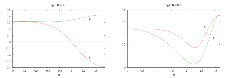
Figure 4: Behavior of $k_{1}$ and $k_{2}$ on marginally DTTSs as functions of the polar angle $\theta$ in the Brill–Lindquist case. Left panel: $k_{1}$ and $k_{2}$ for the common marginally DTTS in the case $z_{0}/GM=1.0$. The relation $k_{1}\leq k_{2}$ is kept on the surface. Right panel: $k_{1}$ and $k_{2}$ for the marginally DTTS that encloses only the upper black hole in the case $z_{0}/GM=0.2$. The relation $k_{1}\geq k_{2}$ is kept on the surface.

Figure 3 shows three-dimensional (3D) plots of the marginally DTTSs for the cases $z_{0}/GM=0.2$ (left panel), $0.8$ (middle panel), and $1.1506$ (right panel). In this figure, two kinds of marginally DTTSs are plotted: one is the common marginally DTTS and the other two are the marginally DTTSs each of which surrounds only one of the two black holes. For small $z_{0}/GM$, the two inner marginally DTTSs cross with each other as shown in the left panel. Therefore, there are cases where two dynamically transversely trapping regions overlap. As $z_{0}/GM$ is increased, the two dynamically transversely trapping regions become separate as shown in the middle and right panels. For $z_{0}/GM\geq 1.1507$, no common DTTS can be found, but two separate marginally DTTSs can always be found.

Figure 4 shows the values of $k_{1}$ and $k_{2}$ as functions of the polar angle $\theta$ for a common DTTS in the initial data with $z_{0}/GM=1.0$ (left panel) and for a DTTS that surrounds only the upper black hole (right panel) in the initial data with $z_{0}/GM=0.2$. Because the equation for a marginally DTTS depends on the sign of $k_{1}-k_{2}$, whether the behavior of $k_{1}$ and $k_{2}$ is consistent with the chosen equation must be checked after the solutions are obtained. For a common DTTS, the relation $k_{1}\leq k_{2}$ is kept, while for a DTTS that surrounds only the upper black hole, the relation $k_{1}\geq k_{2}$ is kept.

4.4 Comparison with marginally trapped surfaces

Figure 5: Sections of common apparent horizons with the $(x,z)$-plane in the Brill–Lindquist initial data for $z_{0}/GM=0.0$, $0.05$, $0.10$, $0.15$, $0.20$, $0.25$, $0.30$, $0.35$, and $0.3830$. For $z_{0}/GM\geq 0.3831$, no common apparent horizon is present. Compare with Fig. 2.

Figure 6: 3D plots of marginally trapped surfaces in the Brill–Lindquist initial data for $z_{0}/GM=0.05$ (left panel), $0.20$ (middle panel), and $0.3830$ (right panel). In each panel, three marginally trapped surfaces are presented: One is the common apparent horizon, and each of the other two is associated with one of the two black holes. Compare with Fig. 3.

In Sect. 2.4 we discussed the similarity between (marginally) DTTSs and (marginally) trapped surfaces. We explore the similarity further in the examples of the Brill–Lindquist initial data. Since the initial data are time symmetric, marginally trapped surfaces coincide with minimal surfaces on which $k=k_{1}+k_{2}=0$ holds, where the formulas for $k_{1}$ and $k_{2}$ are presented in Eqs. (98a)–(99b) in Appendix A. Since the common marginally trapped surface is the outermost one, it is also the (common) apparent horizon. Although there are many works that studied marginally trapped surfaces in the Brill–Lindquist initial data (e.g., Cadez:1974 ; Bishop:1982 ; Gundlach:1997 ; Yoshino:2005 ), including the original work by Brill and Lindquist Brill:1963 , here we present the results generated by our code.

Figure 5 shows the sections of the common apparent horizons with the $(x,z)$-plane for $z_{0}/GM=0.0$, $0.05$, $0.10$, $0.15$, $0.20$, $0.25$, $0.30$, $0.35$, and $0.3830$. For $z_{0}/GM\geq 0.3831$, we could not find a common apparent horizon. For $z_{0}/GM=0.0$, the common apparent horizon is spherically symmetric with the radius $\tilde{r}/GM=1/2$, which corresponds to the horizon radius of a Schwarzschild spacetime in the isotropic coordinates. As the value of $z_{0}/GM$ is increased, the common apparent horizon becomes distorted. By comparing Figs. 2 and 5, a similarity between the two kinds of surfaces can be recognized in the response to the variation of $z_{0}/GM$.

Figure 6 plots the common apparent horizon and the two marginally trapped surfaces each of which is associated with one of the two black holes, for the cases $z_{0}/GM=0.05$ (left panel), $0.2$ (middle panel), and $0.3830$ (right panel). In contrast to the marginally DTTSs, the two inner marginally trapped surfaces do not cross each other. The dynamically transversely trapping regions overlap because they cover larger domains compared to the trapped regions. For $z_{0}/GM\geq 0.3831$ no common apparent horizon can be found, but two separate marginally trapped surfaces can always be found.

Note that the typical size of the circumference of the apparent horizon, $\sim$$4\pi GM$, is smaller than that of the common marginally DTTS, $\sim$$6\pi GM$. Also, the parameter range $0\leq z_{0}/GM\lesssim 0.3830$ where the common apparent horizon is present is much smaller than the range $0\leq z_{0}/GM\lesssim 1.1506$ where the common DTTS is present. These are because an apparent horizon is an indicator for a stronger gravity region compared to a marginally DTTS.

5 Explicit examples in Majumdar–Papapetrou spacetimes

In this section we explicitly construct marginally DTTSs in Majumdar–Papapetrou spacetimes Majumdar:1947 ; Papapetrou:1947 . In Sect. 5.1, we explain the Majumdar–Papapetrou spacetimes and our setups. The equation for solving a marginally DTTS is explained in Sect. 5.2, and numerical results are presented in Sect. 5.3. Comparison with static TTSs is made in Sect. 5.4.

5.1 Setup

A Majumdar–Papapetrou spacetime is a static electrovacuum spacetime with the metric

$$ds^{2}=-U^{-2}dt^{2}+U^{2}(dx^{2}+dy^{2}+dz^{2}),$$ (71)

and an electromagnetic four-potential

$$A_{a}=\frac{U^{-1}}{\sqrt{G}}(\mathrm{d}t)_{a}.$$ (72)

We have two equations from the Einstein field equations, which correspond to the Hamiltonian constraint and the evolution equations, and one equation from Maxwell’s equations. These three equations are reduced to exactly the same form,

$$\bar{\nabla}^{2}U=0,$$ (73)

where $\bar{\nabla}^{2}$ is the flat space Laplacian introduced in Eq. (62). In general, the Majumdar–Papapetrou spacetime represents $N$ extremal black holes at rest. Here, we focus our attention on the two equal-mass black holes, and choose the following solution to this equation,

$$U=1+\frac{GM}{2\tilde{r}_{+}}+\frac{GM}{2\tilde{r}_{-}},$$ (74)

with $\tilde{r}_{\pm}$ defined in Eqs. (64), where $M$ corresponds to the ADM mass. In the case of $z_{0}=0$, this metric represents an extremal Reissner-Nortström spacetime in the isotropic coordinates and $r=0$ corresponds to the horizon. By contrast, in the case of $z_{0}>0$, the metric represents a spacetime with two extremal black holes with horizons located at $(x,y,z)=(0,0,\pm z_{0})$. The two black holes are kept static because the gravitational attraction and the electromagnetic repulsive interaction are balanced.

5.2 The equation for a marginally DTTS

We solve for marginally DTTSs on the slice $t=\mathrm{const.}$ in this spacetime, which is time symmetric. Since the spatial metric in Eq. (71) is conformally flat, the same method for the Brill–Lindquist initial data can be applied to this system. The difference is that there is a nonzero contribution from $P_{r}$ to the equation for marginally DTTSs, Eq. (69), and the conformal factor $\varPsi$ must be replaced by $U^{1/2}$. The detailed forms of the equations are presented in Appendix B.

In contrast to the Brill–Lindquist case, $k_{1}-k_{2}$ changes its sign on marginally DTTSs in this spacetime. For this reason, in solving for a marginally DTTS numerically, we monitor the sign of $k_{1}-k_{2}$ and choose the appropriate equation at each step of the polar angle, $\theta=\theta_{i}:=i\times\Delta\theta$ ($i=0,1,...$), in order to calculate the data at the next step, $\theta=\theta_{i+1}$.

5.3 Numerical results

Figure 7: Sections of common marginally DTTSs with the $(x,z)$-plane in the Majumdar–Papapetrou spacetimes for $z_{0}/GM=0.0$, $0.125$, $0.25$, $0.375$, $0.5$, $0.625$, $0.75$, and $0.79353$. For $z_{0}/GM\geq 0.79354$, no common marginally DTTS is present.

Figure 8: 3D plots of marginally DTTSs in the Majumdar–Papapetrou spacetime for $z_{0}/GM=0.125$ (left panel), $0.5$ (middle panel), and $0.79353$ (right panel). In each panel, three marginally DTTSs are presented: One is the common DTTS, and each of the other two DTTSs encloses only one black hole.

We now show the numerical results. Figure 7 shows the sections of the common marginally DTTSs with the $(x,z)$-plane in the Majumdar–Papapetrou spacetimes for $z_{0}/GM=0.0$, $0.125$, $0.25$, $0.375$, $0.5$, $0.625$, $0.75$, and $0.79353$. For $z_{0}/GM=0.0$, the common marginally DTTS is spherically symmetric with the radius $\tilde{r}/GM=1$. This corresponds to the radius of the photon sphere of an extremal Reissner-Nordström spacetime in the isotropic coordinates. As the value of $z_{0}/GM$ is increased, the common DTTS becomes distorted, and it exists up to $z_{0}/GM\approx 0.79353$. Similarly to the Brill–Lindquist case, for the range $0.647\lesssim z_{0}/GM\lesssim 0.79353$ we could obtain two solutions that correspond to the outer and inner boundaries of a common dynamically transversely trapping region. Around $z_{0}/GM\approx 0.79353$, the inner and outer boundaries degenerate, and the common dynamically transversely trapping region vanishes as $z_{0}/GM$ is further increased.

Figure 8 shows 3D plots of the marginally DTTSs for the cases $z_{0}/GM=0.125$ (left panel), $0.5$ (middle panel), and $0.79353$ (right panel). In this figure, we plot both the common marginally DTTS and the marginally DTTSs, each of which surrounds only one of the two black holes. As shown in the left panel, the two inner marginally DTTSs cross with each other for small $z_{0}/GM$, and the two dynamically transversely trapping regions overlap. As $z_{0}/GM$ is increased, the two dynamically transversely trapping regions become separate as shown in the middle and right panels. Although no common DTTS can be found for $z_{0}/GM\geq 0.79354$, the two separate DTTSs can always be found.

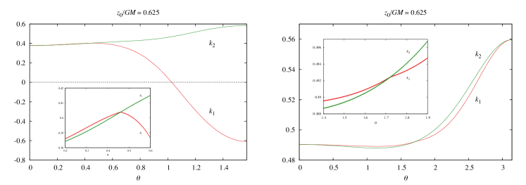
Figure 9: Behavior of $k_{1}$ and $k_{2}$ on marginally DTTSs as functions of the polar angle $\theta$ in the Majumdar–Papapetrou case. Left panel: $k_{1}$ and $k_{2}$ for the common marginally DTTS in the case $z_{0}/GM=0.625$. Right panel: $k_{1}$ and $k_{2}$ for the marginally DTTS that encloses only the upper black hole in the case $z_{0}/GM=0.625$. In both panels, $k_{1}-k_{2}$ changes its sign from positive to negative as $\theta$ is increased. In each of the two panels, the inset enlarges the neighborhood of the point where $k_{1}-k_{2}$ changes its sign.

Figure 9 shows the values of $k_{1}$ and $k_{2}$ as functions of the polar angle $\theta$ for a common DTTS (left panel) and for a DTTS that surrounds only the upper black hole (right panel) for the case $z_{0}/GM=0.625$. In each panel, $k_{1}-k_{2}$ changes its sign at some $\theta=\theta_{\rm c}$, and the equations are changed in the domains $\theta\leq\theta_{\rm c}$ and $\theta_{\rm c}\leq\theta$, accordingly. The curve for $k_{1}$ is bent at $\theta=\theta_{\rm c}$, because, due to the change of the equations, the third derivative of $h(\theta)$ is discontinuous at $\theta=\theta_{\rm c}$. Since $k_{1}$ depends on $h^{\prime\prime}$ as presented in Eqs. (107a) and (108a), the derivative of $k_{1}$ becomes discontinuous, although the curve of $k_{1}$ itself is continuous. By contrast, since $k_{2}$ does not depend on $h^{\prime\prime}$ as presented in Eqs. (107b) and (108b), the curve of $k_{2}$ is not bent at $\theta=\theta_{\rm c}$. These results indicate that the obtained marginal DTTSs are of differentiability class $C^{2}$ in this case.

5.4 Comparison with static TTSs

Since the Majumdar–Papapetrou spacetime is a static spacetime, the static TTSs defined in our previous paper Yoshino:2017 can also be studied. Here, we study common static TTSs that enclose both black holes and compare them with common DTTSs.

A static timelike surface $S$ is said to be a static TTS if and only if arbitrary photons emitted from arbitrary points on $S$ in the tangential direction to $S$ propagate on $S$ or toward the inside of $S$. This condition, hereafter the static TTS condition, is expressed as $\bar{K}_{ab}k^{a}k^{b}\leq 0$, where $k^{a}$ is arbitrary null tangent vectors to $S$. The static TTS condition is rewritten as

$$\mathrm{max}(k_{1},k_{2})\leq\frac{{}^{(3)}\pounds_{\hat{r}}\alpha_{\rm s}}{\alpha_{\rm s}},$$ (75)

on a static slice $t=\mathrm{const.}$, where $\alpha_{\rm s}:=\sqrt{-\xi_{a}\xi^{a}}=U^{-1}$ is the lapse function associated with the timelike Killing vector $\xi^{a}$. Unlike the marginally transversely trapping condition in the DTTS case, we do not require the existence of a photon that marginally satisfies the condition in Eq. (75).

Figure 10: Examples of common static TTSs in the Majumdar–Papapetrou spacetime for $z_{0}/GM=0.1$ (left panel), $0.2$ (middle panel), and $0.272$ (right panel). Two solid curves indicate the contours of $U+2\tilde{r}U_{,\tilde{r}}=0$, and $\tilde{r}=\mathrm{const.}$ surfaces between the two curves are static TTSs, as some of them are indicated by dashed circles.

First, let us consider the condition that a surface $\tilde{r}=\mathrm{const.}$ becomes a common static TTS. The formulas for $k_{1}$ and $k_{2}$ are given in Eqs. (107a)–(108b) in Appendix B. Since $k_{1}=k_{2}=U^{-1}(1/\tilde{r}+U_{,\tilde{r}}/U)$ holds for a surface $\tilde{r}=\mathrm{const.}$, the static TTS condition is reduced to

$$U+2\tilde{r}U_{,\tilde{r}}\leq 0.$$ (76)

Figure 10 shows the contours of $U+2\tilde{r}U_{,\tilde{r}}=0$ in the cases of $z_{0}/GM=0.1$, $0.2$, and $0.272$. All of the surfaces $\tilde{r}=\mathrm{const.}$ between the two contours are common static TTSs, and some of them are indicated by dashed circles. The surfaces $\tilde{r}=\mathrm{const.}$ can become TTSs only if $z_{0}$ is within the range $0\leq z_{0}/GM\leq\sqrt{2/27}\approx 0.2722$. For $\sqrt{2/27}<z_{0}/GM$, the contour surfaces are reconnected and a surface $\tilde{r}=\mathrm{const.}$ cannot cross the equatorial plane without violating the static TTS condition of Eq. (76).

Next, let us consider the general case where a common static TTS is given by $\tilde{r}=h(\tilde{\theta})$. As a necessary condition, a common static TTS must satisfy $k_{2}\leq{}^{(3)}\pounds_{\hat{r}}\alpha_{\rm s}/\alpha_{\rm s}$ on the equatorial plane. Since $\cot\tilde{\theta}=U_{,\tilde{\theta}}=0$ at $\tilde{\theta}=\pi/2$ in Eqs. (107b) and (108b), this necessary condition is reduced to

$$\left.(U+2\tilde{r}U_{,\tilde{r}})\right|_{\tilde{r}=h(\pi/2)}\leq 0,$$ (77)

which is the same as the static TTS condition in Eq. (76) for $\tilde{r}=\mathrm{const.}$ surfaces. Therefore, we find the following: if there is no radius in the equatorial plane that satisfies the condition in Eq. (77), there is no common static TTS. Conversely, if there is a radius in the equatorial plane that satisfies the condition in Eq. (77), common static TTSs are present (for example, the surface $\tilde{r}=\mathrm{const.}$). The condition for the existence of common static TTSs is determined only on the equatorial plane.

Physically, this result is directly related to the (non)existence of circular orbits of photons on the equatorial plane. As studied in Ref. Wunsch:2013 , two circular orbits of photons are located at the radius at which the equality in the condition of Eq. (77) holds. Therefore, if two circular orbits of photons exist, common static TTSs are present because they can cross the equatorial plane at the radius between the two circular orbits of photons. If there are no circular orbits of photons, common static TTSs cannot cross the equatorial plane anymore.

Notice that the parameter range $0\leq z_{0}/GM\lesssim 0.2722$ for the existence of common static TTSs is much smaller than the range $0\leq z_{0}/GM\lesssim 0.7935$ for the existence of common DTTSs. Such difference occurs because the timelike surface $S$ must not change in time in the case of a static TTS, while $S$ is flexible and can change its shape in time in the case of a DTTS. Due to this flexibility of $S$ in the case of a DTTS, even if an area element of $\sigma_{t}$ (defined in Sect. 2.3.1 as a $t=\mathrm{const.}$ slice of $S$) expands in the $\phi$ direction in time, the accelerated contraction condition is not necessarily violated, because ${}^{(3)}\bar{\pounds}_{n}\bar{k}\leq 0$ is satisfied if the area element contracts in the $\theta$ direction sufficiently rapidly. Therefore, the concept of a DTTS is fairly different from that of a static TTS.

6 Penrose-like inequality

In the following two sections, we focus on general properties of DTTSs. In this section we prove that DTTSs satisfy the Penrose-like inequality in Eq. (2) under certain conditions. Before doing this, it is useful to review the Penrose inequality, Eq. (1).

The Penrose inequality (1) is conjectured to be satisfied by an apparent horizon by the following argument. If the cosmic censorship hypothesis holds, there is an event horizon outside the apparent horizon, and the area of the event horizon $A_{\rm EH}$ is expected to be equal to or larger than that of the apparent horizon, i.e. $A_{\rm AH}\leq A_{\rm EH}$. Due to the area theorem, the event horizon has the area $A_{\rm EH}^{\rm(f)}$, larger than $A_{\rm EH}$, after the system settles down to a stationary state described by a Kerr black hole, i.e. $A_{\rm EH}\leq A_{\rm EH}^{\rm(f)}$. Furthermore, the relation $A_{\rm EH}^{\rm(f)}\leq 4\pi(2GM)^{2}$ is expected to be satisfied due to the positivity of the radiated energy of gravitational waves. This leads to the Penrose conjecture, the inequality in Eq. (1). Note that a counterexample to the Penrose conjecture has been constructed in Ref. BenDov:2004 by cutting and gluing Schwarzschild spacetimes and Friedmann universes in a complex manner. In this system, the Penrose inequality is not satisfied because the inequality $A_{\rm AH}\leq A_{\rm EH}$ in the above discussion is violated. However, it is possible to reformulate the Penrose conjecture to be consistent with the above counterexample as argued in Ref. BenDov:2004 .

Although the Penrose conjecture remains an open problem, the Riemannian Penrose inequality, which is a variant of the original Penrose inequality, has been proved. If an asymptotically flat three-dimensional space $\Sigma$ with nonnegative scalar curvature possesses an outermost minimal surface with the area $A_{\rm min}$, the Riemannian Penrose inequality asserts

$$A_{\rm min}\leq 4\pi(2GM)^{2}.$$ (78)

As a corollary, the Riemannian Penrose inequality implies that the original Penrose inequality is satisfied by an apparent horizon in time-symmetric initial data. There are two methods to prove the Riemannian Penrose inequality: the method by the inverse mean curvature flow Wald:1977 ; Huisken:2001 and Bray’s conformal flow Bray:2001 . Of these, the method by the inverse mean curvature flow is directly used in this section.

The inverse mean curvature flow is an example of a geometric flow of hypersurfaces of a Riemannian manifold. Let us consider a flow of two-dimensional hypersurfaces $\sigma(r)$ with spherical topology in $\Sigma$, each of which is labeled by the radial coordinate $r$. If the lapse function $\varphi$ satisfies $\varphi=1/k$, this flow is said to be the inverse mean curvature flow. For each of the surfaces of the flow, Geroch’s quasilocal mass is defined by

$$E(r)=\frac{A^{1/2}}{64\pi^{3/2}G}\left(16\pi-\int_{\sigma(r)}k^{2}dA\right),$$ (79)

where $A$ and $dA$ are the area and the area element of $\sigma(r)$. Geroch’s quasilocal mass is checked to coincide with the ADM mass at spacelike infinity, $r\to\infty$. Furthermore, for a space with nonnegative Ricci scalar, Geroch’s quasilocal mass is proved to satisfy

$$\frac{dE}{dr}\geq 0,$$ (80)

which is called the Geroch monotonicity Geroch:1973 . Due to the Geroch monotonicity, Geroch’s quasilocal mass for the surface $\sigma_{0}=\sigma(0)$, i.e. $r=0$, satisfies $E(0)\leq M$. If the surface $\sigma_{0}$ is an infinitesimal limit of an $S^{2}$ surface, we have

$$E(0)=0\leq M,$$ (81)

which proves the positive energy theorem Geroch:1973 . If the surface $\sigma_{0}$ is a minimal surface on which $k=0$ is satisfied, we have

$$E(0)=\frac{A_{\rm min}^{1/2}}{4\pi^{1/2}G}\leq M.$$ (82)

This implies the Riemannian Penrose inequality of Eq. (78) as pointed out in Ref. Wald:1977 . Note that singularities appear in the inverse mean curvature flow in general. However, Huisken and Ilmanen Huisken:2001 showed that it is possible to introduce a weak solution to the inverse mean curvature flow without breaking the Geroch monotonicity, and thus gave a complete proof of the Riemannian Penrose inequality.

In order to prove that DTTSs satisfy the Penrose-like inequality of Eq. (2), we will show that a DTTS satisfies

$$\int_{\sigma_{0}}k^{2}dA\leq\frac{16}{3}\pi$$ (83)

under certain conditions. Then, the Geroch monotonicity implies that

$$\frac{A_{0}^{1/2}}{6\pi^{1/2}G}\leq E(0)\leq M,$$ (84)

which is equivalent to the Penrose-like inequality in Eq. (2). We discuss the cases of the time-symmetric initial data and the momentarily stationary axisymmetric initial data one by one.

6.1 Time-symmetric initial data

Suppose we have a DTTS $\sigma_{0}$ in time-symmetric initial data $\Sigma$. The DTTS $\sigma_{0}$ satisfies the formula for ${}^{(3)}\bar{\pounds}_{n}\bar{k}$ given by Eq. (48). In this equation, the inequality ${}^{(3)}\bar{\pounds}_{n}\bar{k}\leq 0$ holds from the accelerated contraction condition of Eq. (23). We assume the radial pressure to be nonpositive, $P_{r}\leq 0$. Furthermore, if the convexity $k_{\rm S}\geq 0$ is assumed for the DTTS, we have

$$2kk_{\rm L}+k^{2}-k_{ab}k^{ab}=\frac{3}{2}k^{2}+\frac{1}{2}(k_{\rm L}+3k_{\rm S})(k_{\rm L}-k_{\rm S})\geq\frac{3}{2}k^{2}.$$ (85)

Then, we have the inequality, ${}^{(2)}R\geq(3/2)k^{2}$ and integration over the surface $\sigma_{0}$ gives

$$\int_{\sigma_{0}}k^{2}dA\leq\frac{2}{3}\int_{\sigma_{0}}{}^{(2)}RdA.$$ (86)

If there is a point at which $k>0$ holds, the Gauss–Bonnet theorem tells us that $\sigma_{0}$ has topology $S^{2}$ and satisfies $\int_{\sigma_{0}}{}^{(2)}RdA=8\pi$. Therefore, the inequality in Eq. (83) is satisfied, and thus we have shown the following:

Theorem 1.

A convex DTTS, $\sigma_{0}$, in time-symmetric, asymptotically flat initial data has topology $S^{2}$ and satisfies the Penrose-like inequality $A_{0}\leq 4\pi(3GM)^{2}$ if $P_{r}\leq 0$ holds on $S_{0}$, $k>0$ at least at one point on $S_{0}$, and ${}^{(3)}R$ is nonnegative (i.e. the energy density $\rho\geq 0$) in the outside region.

Note that, by virtue of the inequality in Eq. (85), Theorem 1 also holds for a nonconvex DTTS as well if $k_{\rm S}$ is within the range $0>k_{\rm S}\geq-k_{\rm L}/3$. Although nonpositive radial pressure $P_{r}\leq 0$ may seem strange, it is not very unrealistic because it is satisfied if the spacetime is vacuum around $\sigma_{0}$, and furthermore, the radial pressure due to electromagnetic fields is negative on spherical surfaces in a Reissner–Nordström spacetime.

6.2 Momentarily stationary axisymmetric initial data

In the case of the momentarily stationary axisymmetric initial data, the formula for ${}^{(3)}\bar{\pounds}_{n}\bar{k}$ is given by Eq. (59). Similarly to the time-symmetric case, the accelerated contraction condition implies that ${}^{(3)}\bar{\pounds}_{n}\bar{k}\leq 0$, and $P_{r}\leq 0$ is assumed. Assuming $\sigma_{0}$ to be a convex surface with $k_{\rm S}\geq 0$, the relation $2k{}^{(3)}\pounds_{\hat{r}}\alpha/\alpha\geq 2kk_{\rm L}$ holds from the inequality in Eq. (58) and $k\geq 0$, and thus we have

$$2k\frac{{}^{(3)}\pounds_{\hat{r}}\alpha}{\alpha}+k^{2}-k_{ab}k^{ab}\geq\frac{3}{2}k^{2},$$ (87)

by the same calculation as Eq. (85). Since it is difficult to control the sign of $({}^{(3)}\pounds_{\hat{r}}\tilde{\omega})^{2}-(\mathcal{D}\tilde{\omega})^{2}$, we simply assume that $({}^{(3)}\pounds_{\hat{r}}\tilde{\omega})^{2}\geq(\mathcal{D}\tilde{\omega})^{2}$. In other words, we choose surfaces $\sigma_{0}$ so that this condition is satisfied. Then, we have the inequality ${}^{(2)}R\geq(3/2)k^{2}$, and with the same argument as the time-symmetric case, the inequality in Eq. (83) is satisfied. Therefore, we have shown the following:

Theorem 2.

An axisymmetric convex DTTS $\sigma_{0}$ in momentarily stationary axisymmetric initial data has topology $S^{2}$ and satisfies the Penrose-like inequality $A_{0}\leq 4\pi(3GM)^{2}$ if $P_{r}\leq 0$ and

$$({}^{(3)}\pounds_{\hat{r}}\tilde{\omega})^{2}\geq(\mathcal{D}\tilde{\omega})^{2}$$ (88)

hold on $\sigma_{0}$, $k>0$ at least at one point on $\sigma_{0}$, and ${}^{(3)}R$ is nonnegative in the outside region.

Similarly to the time-symmetric case, Theorem 2 also holds for a nonconvex DTTS as well if $k_{\rm S}$ is within the range $0>k_{\rm S}\geq-k_{\rm L}/3$ due to the inequalities in Eqs. (85) and (87).

7 Connection to loosely trapped surfaces

Lastly, we study the connection between DTTSs and LTSs. The LTS is defined in our previous paper Shiromizu:2017 as a surface on which $k>0$ and ${}^{(3)}\pounds_{\hat{r}}k\geq 0$ are satisfied in a flow of two-dimensional closed surfaces in a spacelike hypersurface $\Sigma$. In fact, such surfaces are located only between the horizon $r=2GM$ and the photon surface $r=3GM$ in the Schwarzschild case. It was also proved in Ref. Shiromizu:2017 that an LTS satisfies the inequality in Eq. (83), and hence satisfies the Penrose-like inequality, Eq. (2), if $\Sigma$ has a nonnegative Ricci scalar, ${}^{(3)}R\geq 0$. In Ref. Shiromizu:2017 , clarifying the relation of LTSs to the behavior of photons was left as a remaining problem, and we show here the fact that a DTTS is an LTS at the same time under certain conditions.

We derive a formula that relates ${}^{(3)}\bar{\pounds}_{n}\bar{k}$ and ${}^{(3)}\pounds_{\hat{r}}k$. The trace of the Ricci equation on $\sigma_{0}$ as a hypersurface in $\Sigma$ is

$${}^{(3)}{\pounds}_{\hat{r}}{k}=-{}^{(3)}{R}_{ab}\hat{r}^{a}\hat{r}^{b}-k_{ab}k^{ab}-\frac{1}{\varphi}\mathcal{D}^{2}\varphi,$$ (89)

where ${}^{(3)}{R}_{ab}$ is the Ricci tensor associated with the metric $q_{ab}$ induced on $\Sigma$. This equation is rewritten with the double trace of the Gauss equation of $\sigma_{0}$ in $\Sigma$,

$${}^{(2)}R={}^{(3)}{R}-2{}^{(3)}{R}_{ab}\hat{r}^{a}\hat{r}^{b}+k^{2}-k_{ab}k^{ab},$$ (90)

and the double trace of the Gauss equation on $\Sigma$ in the spacetime $\mathcal{M}$,

$${}^{(3)}R=2G_{ab}n^{a}n^{b}-K^{2}+K_{ab}K^{ab}.$$ (91)

The result is

$${}^{(3)}{\pounds}_{\hat{r}}k=\frac{1}{2}{}^{(2)}R-8\pi G\rho+\frac{1}{2}\left(K^{2}-K_{ab}K^{ab}-k^{2}-k_{ab}k^{ab}\right)-\frac{1}{\varphi}\mathcal{D}^{2}\varphi,$$ (92)

where the Einstein field equations are assumed. Adding Eqs. (40) and (92) and rewriting with the decomposed forms in Eqs. (33) and (42) of $\bar{K}_{ab}$ and $K_{ab}$, respectively, we have

$${}^{(3)}{\pounds}_{\hat{r}}k=-{}^{(3)}\bar{\pounds}_{n}\bar{k}-8\pi G(\rho+P_{r})+k\frac{{}^{(3)}\pounds_{\hat{r}}\alpha}{\alpha}-k_{ab}k^{ab}-\frac{1}{\varphi}\mathcal{D}^{2}\varphi-\bar{k}_{ab}\bar{k}^{ab}\\ +\bar{k}\frac{{}^{(3)}\bar{\pounds}_{n}\varphi}{\varphi}+\frac{1}{\alpha}\mathcal{D}^{2}\alpha.$$ (93)

We apply this formula to a DTTS $\sigma_{0}$. The last two terms vanish because $\alpha=\mathrm{const.}$ and $\bar{k}=0$ are required. Let us evaluate the sign of each term on the right-hand side of Eq. (93). The first term is nonnegative, $-{}^{(3)}\bar{\pounds}_{n}\bar{k}\geq 0$, from the accelerated contraction condition of Eq. (23). The second term is nonpositive as long as the dominant energy condition holds. For this reason, we require $\rho+P_{r}=0$ in order to make the left-hand side positive definite. As for the third and fourth terms, for both of the time-symmetric and momentarily stationary axisymmetric initial data, we have

$$k\frac{{}^{(3)}\pounds_{\hat{r}}\alpha}{\alpha}-k_{ab}k^{ab}\geq kk_{\rm L}-k_{ab}k^{ab}=k_{\rm S}(k_{\rm L}-k_{\rm S})\geq 0$$ (94)

for a convex DTTS with $k_{\rm S}\geq 0$, using the marginally transversely trapping conditions in the time-symmetric and momentarily stationary axisymmetric cases, Eqs. (47) and (57), respectively. We set the fifth term to be zero by choosing $\varphi=\mathrm{const.}$, since $\sigma_{0}$ becomes an LTS if ${}^{(3)}\pounds_{\hat{r}}k\geq 0$ is satisfied at least for one chice of $\varphi$. We discuss the sixth term $-\bar{k}_{ab}\bar{k}^{ab}$ in the time-symmetric and momentarily stationary axisymmetric cases separately.

7.1 Time-symmetric initial data

Since $\bar{k}_{ab}=0$ holds for time-symmetric initial data, ${}^{(3)}{\pounds}_{\hat{r}}{k}\geq 0$ is guaranteed only with the conditions discussed above. Therefore, we have found the following proposition:

Proposition 1.

A convex DTTS $\sigma_{0}$ with $k>0$ in time-symmetric initial data is an LTS as well if $\rho+P_{r}=0$ is satisfied on $\sigma_{0}$.

7.2 Momentarily stationary axisymmetric initial data

For momentarily stationary axisymmetric initial data, $\bar{k}_{ab}$ is given by Eq. (53), and the sixth term becomes

$$-{\bar{k}_{ab}}{\bar{k}^{ab}}=-\frac{\phi_{a}\phi^{a}}{2\tilde{\alpha}^{2}}(\mathcal{D}\tilde{\omega})^{2}\leq 0.$$ (95)

In order to make this term vanish, we have to require $\mathcal{D}_{a}\tilde{\omega}=0$. This means that we limit our discussion to $\tilde{\omega}=\mathrm{const.}$ surfaces:

Proposition 2.

If a contour surface of $\tilde{\omega}$ in momentarily stationary axisymmetric initial data is a convex DTTS on which $\rho+P_{r}=0$ is satisfied, it is an LTS as well.

8 Summary and discussion

In this paper, we have defined a (marginally) dynamical transversely trapping surface (DTTS) as an extended concept of the photon sphere, intending to provide a new theoretical tool to advance our understanding of the properties of dynamically evolving spacetimes with strong gravity regions. The definition is given in Sect. 2.2. Intuitively, a DTTS is a two-dimensional closed surface on a spacelike hypersurface $\Sigma$ such that photons emitted from it in the transverse directions experience accelerated contraction during the propagation affected by strong gravity. The key quantity is ${}^{(3)}\bar{\pounds}_{\bar{n}}\bar{k}$, which is required to be nonpositive by the accelerated contraction condition. This quantity is found from the study on a photon surface in a Schwarzschild spacetime (Sect. 2.1). As discussed in Sects. 2.3.3 and 5.4, the concept of DTTSs is different from that of static/stationary TTSs, which was proposed as surfaces to characterize strong gravity regions in static/stationary spacetimes in our previous paper Yoshino:2017 . These two concepts must be distinguished.

We have prepared the method of solving for a marginally DTTS in the time-symmetric initial data and the momentarily stationary axisymmetric initial data (Sect. 3). By constructing numerical solutions explicitly for systems of two equal-mass black holes in the Brill–Lindquist initial data (Sect. 4) and in the Majumdar–Papapetrou spacetimes (Sect. 5), we have shown that a marginally DTTS is a well-defined concept. Extending the method to other configurations is necessary, and we plan to study this issue in a forthcoming paper.

Marginally DTTSs are defined with the intention to make them analogous to marginally trapped surfaces, and we have stressed various aspects of such similarity. Both surfaces are determined on a given spacelike hypersurface $\Sigma$, and have similar gauge-independent and -dependent features as discussed in Sect. 2.4. In the Brill–Lindquist initial data, their shapes and dependence on the system parameter $z_{0}/GM$ show qualitatively similar behavior (Sects. 4.3 and 4.4). Furthermore, we have shown that the area of a DTTS satisfies the Penrose-like inequality in Eq. (2) under certain conditions in Sect. 6, similarly to the area of a marginally trapped surface being conjectured (and partly proved) to satisfy the Penrose inequality in Eq. (1). In addition, in Sect. 7 we have discussed the fact that DTTSs are connected to LTSs proposed in our previous paper Shiromizu:2017 under some situations.

Further similarity between marginally DTTSs and marginally trapped surfaces could be explored. For example, as the condition for the formation of apparent horizons, the hoop conjecture Thorne:1972 has been proposed: “Black holes with horizons form when and only when a mass $M$ gets compacted into a region whose circumference in every direction is bounded by $C\lesssim 2\pi(2GM)$.” Although no solid proof has been found up to now, this conjecture is checked to be satisfied in various situations (e.g. Chiba:1994 ; Yoshino:2001 ; Yoshino:2007 ). One of the implications of this conjecture is that the apparent horizon cannot become arbitrarily long in one direction. The analogous condition, $C\lesssim 2\pi(3GM)$, may be expected to hold for the formation of marginally DTTSs. We are planning to study this issue in future.

The concept of a trapped surface has become important through the singularity theorems (see pp. 239–241 of Ref. Wald ). Assuming cosmic censorship, the existence of a trapped surface implies the presence of an event horizon outside. Therefore, the existence of a trapped surface strongly restricts the global property of a spacetime. Does the existence of a DTTS restrict the global structure of a spacetime as well? Unfortunately, this is unlikely under broad assumptions because studies on a spherically symmetric barotropic star do not necessarily exclude a star with radius smaller than $3GM$ as general arguments Buchdahl:1959 ; Barraco:2002 ; Fujisawa:2015 . However, a detailed numerical study indicates that the radii of spherical polytropic stars cannot be smaller than $3GM$ Saida:2015 , and therefore, for restricted situations, the presence of a DTTS may result in the formation of an event horizon. This issue is worth challenging. Note that, since photons in the definition of a DTTS are emitted in transverse directions, a collection of corresponding null geodesics is not an ordinary null geodesic congruence. For this reason, a new technology to handle the propagation of such photons should be required. Related to this issue, a “wandering set” was recently proposed as an extension of a photon sphere, $r=3GM$ in the Schwarzschild case, from the global point of view Siino:2019 . Since a wandering set would be an analogous concept to an event horizon as a generalization of the horizon, $r=2GM$ in the Schwarzschild case, the concepts of DTTSs and a wandering set may be related to each other like trapped surfaces and an event horizon are related by the singularity theorems. It would be interesting to explore such a connection.

Finally, we point out the important difference between DTTSs and trapped surfaces (or apparent horizons). On one hand, positions at which trapped surfaces exist cannot be observed in principle since they are formed within an event horizon, unless cosmic censorship or the null energy condition is violated. On the other hand, since DTTSs are formed and remain outside the event horizon, positions at which DTTSs exist are observable. For this reason, we expect that the concept of DTTSs would also become important in the context of observations of strong gravity regions in dynamical evolutions.

H.Y. thanks Hideki Ishihara and Ken-ichi Nakao for helpful comments. H.Y. is supported by the Grant-in-Aid for Scientific Research (C) No. JP18K03654 from the Japan Society for the Promotion of Science (JSPS). K. I. is supported by JSPS Grant-in-Aid for Young Scientists (B) No. JP17K14281. T. S. is supported by Grant-in-Aid for Scientific Research (C) No. JP16K05344 from JSPS. K.I. and T.S. are also supported by Scientific Research (A) No. JP17H01091 and 
in part by JSPS Bilateral Joint Research Projects (JSPS-NFR collaboration) “String Axion Cosmology.” The work of H.Y. is partly supported by Osaka City University Advanced Mathematical Institute (MEXT Joint Usage/Research Center on Mathematics and Theoretical Physics).

Appendix A Equations for marginally DTTSs in the Brill–Lindquist initial data

In this appendix we derive the equations for marginally DTTSs in the Brill–Lindquist initial data studied in Sect. 4.

In Eqs. (66a) and (66b), the coordinates $(r,\theta)$ are introduced. Transforming the metric from $(\tilde{r},\tilde{\theta},\phi)$ coordinates to $(r,\theta,\phi)$ coordinates, we have the nonzero components

$$\varphi^{2} = \varPsi^{4}\left[1+(r+h)^{2}p_{,r}^{2}\right],$$ (96a)

$$\gamma_{r\theta} = \varPsi^{4}\left[h^{\prime}-(r+h)^{2}(1-p_{,\theta})p_{,r}\right]$$ (96b)

$$h_{\theta\theta} = \varPsi^{4}\left[h^{\prime 2}+(r+h)^{2}(1-p_{,\theta})^{2}\right],$$ (96c)

$$h_{\phi\phi} = \varPsi^{4}(r+h)^{2}\sin^{2}\tilde{\theta},$$ (96d)

in the spatial part of the metric in Eq. (29). We determine the function $p(r,\theta)$ so that $(r,\theta)$ become orthogonal, i.e. $\gamma_{r\theta}=0$. On $\sigma_{0}$ (that is, $r=0$), this means

$$\left.p_{,r}\right|_{\sigma_{0}}=\frac{h^{\prime}}{h^{2}},\qquad\left.p_{,r\theta}\right|_{\sigma_{0}}=\frac{h^{\prime\prime}}{h^{2}}-\frac{2h^{\prime 2}}{h^{3}},$$ (97)

because $p_{,\theta}=p_{,\theta\theta}=0$ holds on $\sigma_{0}$. In the coordinates $(r,\theta,\phi)$, the coordinate components of the extrinsic curvature $k_{ab}$ are calculated by $k_{ij}=h_{ij,r}/2\varphi$ on $\sigma_{0}$, and the orthonormal components $k_{1}$ and $k_{2}$ are given by $k_{1}=k_{\theta\theta}/h_{\theta\theta}$ and $k_{2}=k_{\phi\phi}/h_{\phi\phi}$. The result is

$$k_{1} = -\frac{h}{\varPsi^{2}(h^{2}+h^{\prime 2})^{3/2}}(h^{\prime\prime}+C),$$ (98a)

$$k_{2} = \frac{D}{\varPsi^{2}h\sqrt{h^{2}+h^{\prime 2}}},$$ (98b)

with

$$C = -h-2\frac{h^{\prime 2}}{h}-2\left(\frac{\varPsi_{,\tilde{r}}}{\varPsi}-\frac{h^{\prime}}{h^{2}}\frac{\varPsi_{,\tilde{\theta}}}{\varPsi}\right)\left(h^{2}+h^{\prime 2}\right),$$ (99a)

$$D = h-\cot\theta h^{\prime}+2\left(\frac{\varPsi_{,\tilde{r}}}{\varPsi}-\frac{h^{\prime}}{h^{2}}\frac{\varPsi_{,\tilde{\theta}}}{\varPsi}\right)h^{2}.$$ (99b)

From the induced metric in Eq. (67) on $\sigma_{0}$, the Ricci scalar ${}^{(2)}R$ is calculated as

$$\frac{1}{2}{}^{(2)}R=\frac{1}{\varPsi^{4}(h^{2}+h^{\prime 2})}\left(Ah^{\prime\prime}+B\right),$$ (100)

with

$$A=-\frac{2\varPsi_{,\tilde{r}}}{\varPsi}+\frac{1}{h^{2}+h^{\prime 2}}\left(2\frac{\varPsi_{,\tilde{r}}h^{\prime}+\varPsi_{,\tilde{\theta}}}{\varPsi}h^{\prime}-h\right)+\frac{h^{\prime}}{h^{2}+h^{\prime 2}}\cot\theta,$$ (101a)

$$B=1-\frac{2}{\varPsi}\left[\varPsi_{,\tilde{r}\tilde{r}}h^{\prime 2}+2\varPsi_{,\tilde{r}\tilde{\theta}}h^{\prime}+\varPsi_{,\tilde{\theta}\tilde{\theta}}-\frac{(\varPsi_{,\tilde{r}}h^{\prime}+\varPsi_{,\tilde{\theta}})^{2}}{\varPsi}\right]\\ -\frac{h^{\prime 2}}{h(h^{2}+h^{\prime 2})}\left(2\frac{\varPsi_{,\tilde{r}}h^{\prime}+\varPsi_{,\tilde{\theta}}}{\varPsi}h^{\prime}-h\right)-\left[\frac{h^{\prime}}{h^{2}+h^{\prime 2}}\left(h+2\frac{h^{\prime 2}}{h}\right)+2\frac{\varPsi_{,\tilde{r}}h^{\prime}+\varPsi_{,\tilde{\theta}}}{\varPsi}\right]\cot\theta.$$ (101b)

Below, we study the equation for a marginally DTTS, Eq. (69), for the cases $k_{1}\leq k_{2}$ and $k_{1}\geq k_{2}$, separately.

A.1 The case $k_{1}\leq k_{2}$

In the case $k_{1}\leq k_{2}$, we put $\mathrm{max}(k_{1},k_{2})=k_{2}$ in Eq. (69), which reduces to

$$h^{\prime\prime}=\frac{-2CD+(D^{2}/h^{2}-B)(h^{2}+h^{\prime 2})}{2D+A(h^{2}+h^{\prime 2})}.$$ (102)

in the range $0<\theta<\pi$. Since Eq. (102) includes $\cot\theta$, we have to regularize the equation at the poles $\theta=0$ and $\pi$. Since $h^{\prime}=0$ and $\varPsi_{,\tilde{\theta}}=0$ holds at the poles for axisymmetric initial data and an axisymmetric surface, the terms including $\cot{\tilde{\theta}}$ behave as $h^{\prime}\cot\theta\to h^{\prime\prime}$ and $\varPsi_{,\tilde{\theta}}\cot\theta\to\varPsi_{,\tilde{\theta}\tilde{\theta}}$ in the limit $\theta\to 0$ and $\pi$. Then, a quadratic equation for $h^{\prime\prime}$ is derived as

$$2h^{\prime\prime 2}+4\tilde{C}h^{\prime\prime}+3\tilde{C}^{2}=h^{2}\left(1-\frac{4\varPsi_{,\tilde{\theta}\tilde{\theta}}}{\varPsi}\right),$$ (103)

where $\tilde{C}=-(2h^{2}\varPsi_{,\tilde{r}}/\varPsi+h)$ is the value of $C$ at the poles. Then, a solution with double sign is obtained for $h^{\prime\prime}$, and we must choose a physically appropriate sign. This can be done by considering the spherically symmetric case $z_{0}=0$, because $h=(1+\sqrt{3}/2)GM$ is a solution and the sign must be chosen so that $h^{\prime\prime}=0$ is realized. In this way, we obtain

$$h^{\prime\prime}=h+2\frac{\varPsi_{,\tilde{r}}}{\varPsi}h^{2}-\frac{\sqrt{2}h}{\varPsi}\sqrt{-\left[\varPsi\varPsi_{,\tilde{\theta}\tilde{\theta}}+\varPsi_{,\tilde{r}}h(\varPsi+\varPsi_{,\tilde{r}}h)\right]},$$ (104)

for $\theta=0$ and $\pi$.

A.2 The case $k_{1}\geq k_{2}$

In the case $k_{1}\geq k_{2}$, we set $\mathrm{max}(k_{1},k_{2})=k_{1}$ in Eq. (69). Then, the equation is reduced to

$$h^{\prime\prime 2}+2\left[C-\frac{h^{2}+h^{\prime 2}}{h^{2}}D-\frac{(h^{2}+h^{\prime 2})^{2}}{2h^{2}}A\right]h^{\prime\prime}+C^{2}-2\frac{h^{2}+h^{\prime 2}}{h^{2}}CD-\frac{(h^{2}+h^{\prime 2})^{2}}{h^{2}}B=0.$$ (105)

Solving this equation with respect to $h^{\prime\prime}$, a solution with double sign is obtained. An appropriate sign is chosen by requiring that $h^{\prime\prime}=0$ is realized in the spherically symmetric case. The result is

$$h^{\prime\prime}=-C+\frac{h^{2}+h^{\prime 2}}{h^{2}}\left[D+\frac{1}{2}(h^{2}+h^{\prime 2})A\right]-\frac{h^{2}+h^{\prime 2}}{h^{2}}\sqrt{\left[D+\frac{1}{2}(h^{2}+h^{\prime 2})A\right]^{2}+h^{2}(B-AC)},$$ (106)

for $0<\theta<\pi$. At the poles $\theta=0$ and $\pi$, the regularized equation is reduced to the same equation as the case $k_{1}\leq k_{2}$, Eq. (104), because $k_{1}=k_{2}$ is satisfied at the poles by regular surfaces.

Appendix B Equations for marginally DTTSs in the Majumdar–Papapetrou spacetime

The equations for marginally DTTSs in the Majumdar–Papapetrou spacetime are obtained by the same basic procedure as the Brill–Lindquist case. We span the spherical-polar coordinates $(\tilde{r},\tilde{\theta},\phi)$, parametrize the surface $\sigma_{0}$ as $\tilde{r}=h(\tilde{\theta})$, and introduce the coordinates $(r,\theta,\phi)$ in the same manner as the Brill–Lindquist case. The geometrical quantities on $t=\mathrm{const.}$ are obtained by replacing $\varPsi$ with $U^{1/2}$ in the Brill–Lindquist cases given in Appendix A. Then, the formulas for $k_{1}$ and $k_{2}$ are

$$k_{1} = -\frac{h}{U(h^{2}+h^{\prime 2})^{3/2}}(h^{\prime\prime}+C),$$ (107a)

$$k_{2} = \frac{D}{Uh\sqrt{h^{2}+h^{\prime 2}}},$$ (107b)

with

$$C = -h-2\frac{h^{\prime 2}}{h}-\left(\frac{U_{,\tilde{r}}}{U}-\frac{h^{\prime}}{h^{2}}\frac{U_{,\tilde{\theta}}}{U}\right)\left(h^{2}+h^{\prime 2}\right),$$ (108a)

$$D = h-\cot\theta h^{\prime}+\left(\frac{U_{,\tilde{r}}}{U}-\frac{h^{\prime}}{h^{2}}\frac{U_{,\tilde{\theta}}}{U}\right)h^{2},$$ (108b)

and the formula for ${}^{(2)}R$ is

$$\frac{1}{2}{}^{(2)}R=\frac{1}{U^{2}(h^{2}+h^{\prime 2})}\left(Ah^{\prime\prime}+B_{1}\right),$$ (109)

with

$$A=-\frac{U_{,\tilde{r}}}{U}+\frac{1}{h^{2}+h^{\prime 2}}\left(\frac{U_{,\tilde{r}}h^{\prime}+U_{,\tilde{\theta}}}{U}h^{\prime}-h\right)+\frac{h^{\prime}}{h^{2}+h^{\prime 2}}\cot\theta,$$ (110a)

$$B_{1}=1-\frac{1}{U}\left[U_{,\tilde{r}\tilde{r}}h^{\prime 2}+2U_{,\tilde{r}\tilde{\theta}}h^{\prime}+U_{,\tilde{\theta}\tilde{\theta}}-\frac{(U_{,\tilde{r}}h^{\prime}+U_{,\tilde{\theta}})^{2}}{U}\right]\\ -\frac{h^{\prime 2}}{h(h^{2}+h^{\prime 2})}\left(\frac{U_{,\tilde{r}}h^{\prime}+U_{,\tilde{\theta}}}{U}h^{\prime}-h\right)-\left[\frac{h^{\prime}}{h^{2}+h^{\prime 2}}\left(h+2\frac{h^{\prime 2}}{h}\right)+\frac{U_{,\tilde{r}}h^{\prime}+U_{,\tilde{\theta}}}{U}\right]\cot\theta.$$ (110b)

The important difference is that there is a nonzero contribution from the radial pressure $P_{r}$. The energy-momentum tensor of electromagnetic fields is given by

$$T_{ab}=\frac{1}{4\pi}\left({F_{a}}^{c}F_{bc}-\frac{1}{4}g_{ab}F_{cd}F^{cd}\right),$$ (111)

with the electromagnetic tensor $F_{ab}=\nabla_{a}A_{b}-\nabla_{b}A_{a}$. The spatial components of the energy-momentum tensor, $S_{ab}={q_{a}}^{c}{q_{b}}^{d}T_{cd}$, are calculated as

$$S_{ab}=\frac{1}{4\pi G}\left[-\frac{D_{a}UD_{b}U}{U^{2}}+\frac{1}{2}q_{ab}\frac{(DU)^{2}}{U^{2}}\right]$$ (112)

from Eq. (72), and thus we have

$$8\pi GP_{r}=\frac{(D_{a}U)(D^{a}U)}{U^{2}}-2\frac{(\hat{r}^{a}D_{a}U)^{2}}{U^{2}}=\frac{B_{2}}{U^{2}(h^{2}+h^{\prime 2})},$$ (113)

with

$$B_{2}=(h^{2}+h^{\prime 2})\left(\frac{U_{,\tilde{r}}^{2}}{U^{2}}+\frac{U_{,\tilde{\theta}}^{2}}{h^{2}U^{2}}\right)-2h^{2}\left(\frac{U_{,\tilde{r}}}{U}-\frac{h^{\prime}}{h^{2}}\frac{U_{,\tilde{\theta}}}{U}\right)^{2},$$ (114)

where we used the fact that the components of $\hat{r}^{a}$ in the $(t,\tilde{r},\tilde{\theta},\phi)$ coordinates are given by

$$\hat{r}^{\mu}=\frac{1}{U\sqrt{1+h^{\prime 2}/h^{2}}}\left(0,1,-h^{\prime}/h^{2},0\right)$$ (115)

on $\sigma_{0}$. Defining

$$B=B_{1}+B_{2},$$ (116)

the equation for a marginally DTTS is given by the same form as Eq. (102) in the case $k_{1}\leq k_{2}$, and by the same form as Eq. (106) in the case $k_{1}\geq k_{2}$, in the range $0<\theta<\pi$. At the poles, the equation is regularized as

$$h^{\prime\prime}=\frac{h}{U}\left[U+hU_{,\tilde{r}}-\sqrt{-\left[UU_{,\tilde{\theta}\tilde{\theta}}+hU_{,\tilde{r}}(U+hU_{,\tilde{r}})\right]}\right].$$ (117)

References

- (1) V. Cardoso, A. S. Miranda, E. Berti, H. Witek and V. T. Zanchin, Phys. Rev. D 79, 064016 (2009) [arXiv:0812.1806 [hep-th]].
- (2) B. P. Abbott et al. [LIGO Scientific and Virgo Collaborations], Phys. Rev. Lett. 116, 061102 (2016) [arXiv:1602.03837 [gr-qc]].
- (3) K. S. Virbhadra and G. F. R. Ellis, Phys. Rev. D 62, 084003 (2000) [astro-ph/9904193].
- (4) P. V. P. Cunha, C. A. R. Herdeiro and E. Radu, Phys. Rev. D 96, 024039 (2017) [arXiv:1705.05461 [gr-qc]].
- (5) K. Akiyama et al. [Event Horizon Telescope Collaboration], Astrophys. J. 875, L1 (2019) [arXiv:1906.11238 [astro-ph.GA]].
- (6) R. Wald, General Relativity (Chicago, The University of Chicago Press, 1984).
- (7) C. M. Claudel, K. S. Virbhadra and G. F. R. Ellis, J. Math. Phys. 42, 818 (2001) [gr-qc/0005050].
- (8) C. Cederbaum, arXiv:1406.5475 [math.DG].
- (9) C. Cederbaum and G. J. Galloway, arXiv:1504.05804 [math.DG].
- (10) S. Yazadjiev and B. Lazov, Classical Quantum Gravity 32, 165021 (2015) [arXiv:1503.06828 [gr-qc]].
- (11) C. Cederbaum and G. J. Galloway, Classical Quantum Gravity 33, 075006 (2016) [arXiv:1508.00355 [math.DG]].
- (12) S. S. Yazadjiev, Phys. Rev. D 91, 123013 (2015) [arXiv:1501.06837 [gr-qc]].
- (13) S. Yazadjiev and B. Lazov, Phys. Rev. D 93, 083002 (2016) [arXiv:1510.04022 [gr-qc]].
- (14) M. Rogatko, Phys. Rev. D 93, 064003 (2016) [arXiv:1602.03270 [hep-th]].
- (15) H. Yoshino, Phys. Rev. D 95, 044047 (2017) [arXiv:1607.07133 [gr-qc]].
- (16) Y. Tomikawa, T. Shiromizu and K. Izumi, Prog. Theor. Exp. Phys. 2017, 033E03 (2017) [arXiv:1612.01228 [gr-qc]].
- (17) Y. Tomikawa, T. Shiromizu and K. Izumi, Class. Quant. Grav. 34, 155004 (2017) [arXiv:1702.05682 [gr-qc]].
- (18) G. W. Gibbons and C. M. Warnick, Phys. Lett. B 763, 169 (2016) [arXiv:1609.01673 [gr-qc]].
- (19) Y. Koga and T. Harada, Phys. Rev. D 94, 044053 (2016) [arXiv:1601.07290 [gr-qc]].
- (20) A. A. Shoom, Phys. Rev. D 96, 084056 (2017) [arXiv:1708.00019 [gr-qc]].
- (21) Y. Koga and T. Harada, Phys. Rev. D 98, 024018 (2018) [arXiv:1803.06486 [gr-qc]].
- (22) Y. Koga, Phys. Rev. D 99, 064034 (2019) [arXiv:1901.02592 [gr-qc]].
- (23) Y. Koga and T. Harada, Phys. Rev. D 100, 064040 (2019) [arXiv:1907.07336 [gr-qc]].
- (24) T. Shiromizu, Y. Tomikawa, K. Izumi and H. Yoshino, Prog. Theor. Exp. Phys. 2017, 033E01 (2017) [arXiv:1701.00564 [gr-qc]].
- (25) H. Yoshino, K. Izumi, T. Shiromizu and Y. Tomikawa, Prog. Theor. Exp. Phys. 2017, 063E01 (2017) [arXiv:1704.04637 [gr-qc]].
- (26) R. Penrose, Annals N. Y. Acad. Sci. 224, 125 (1973).
- (27) S. Hod, Phys. Lett. B 727, 345 (2013) [arXiv:1701.06587 [gr-qc]].
- (28) D. V. Gal’tsov and K. V. Kobialko, Phys. Rev. D 99, 084043 (2019) [arXiv:1901.02785 [gr-qc]].
- (29) D. V. Gal’tsov and K. V. Kobialko, arXiv:1906.12065 [gr-qc].
- (30) D. R. Brill and R. W. Lindquist, Phys. Rev. 131, 471 (1963).
- (31) S. D. Majumdar, Phys. Rev. 72, 390 (1947).
- (32) A. Papapetrou, Proceedings of the Royal Irish Academy, Section A 51, 191 (1947).
- (33) S. E. Gralla, D. E. Holz and R. M. Wald, Phys. Rev. D 100, 024018 (2019) [arXiv:1906.00873 [astro-ph.HE]].
- (34) S. A. Hayward, Phys. Rev. D 49, 6467 (1994) [gr-qc/9303006].
- (35) K. i. Nakao, M. Kimura, T. Harada, M. Patil and P. S. Joshi, Phys. Rev. D 90, 124079 (2014) [arXiv:1406.6798 [gr-qc]].
- (36) A. Čadež, Annals Phys. 83, 449 (1974).
- (37) N. T. Bishop, Gen. Rel. Grav. 14, 817 (1982).
- (38) C. Gundlach, Phys. Rev. D 57, 863 (1998) [gr-qc/9707050].
- (39) H. Yoshino, T. Shiromizu and M. Shibata, Phys. Rev. D 72, 084020 (2005) [gr-qc/0508063].
- (40) A. Wunsch, T. Müller, D. Weiskopf and G. Wunner, Phys. Rev. D 87, 024007 (2013) [arXiv:1301.7560 [gr-qc]].
- (41) I. Ben-Dov, Phys. Rev. D 70, 124031 (2004) [gr-qc/0408066].
- (42) P. S. Jang and R. M. Wald, J. Math. Phys. 18, 41 (1977).
- (43) G. Huisken and T. Ilmanen, J. Diff. Geom. 59, 353 (2001).
- (44) H. Bray, J. Diff. Geom. 59, 177 (2001).
- (45) R. Geroch, Ann. N.Y. Acad. Sci. 224, 108 (1973).
- (46) K. S. Thorne, in Magic without Magic: John Archbald Wheeler, edited by J.Klauder (Freeman, San Francisco, 1972).
- (47) T. Chiba, T. Nakamura, K. i. Nakao and M. Sasaki, Class. Quant. Grav. 11, 431 (1994).
- (48) H. Yoshino, Y. Nambu and A. Tomimatsu, Phys. Rev. D 65, 064034 (2002) [gr-qc/0109016].
- (49) H. Yoshino, Phys. Rev. D 77, 041501 (2008) [arXiv:0712.3907 [gr-qc]].
- (50) H. A. Buchdahl, Phys. Rev. 116, 1027 (1959).
- (51) D. Barraco and V. H. Hamity, Phys. Rev. D 65, 124028 (2002).
- (52) A. Fujisawa, H. Saida, C. M. Yoo and Y. Nambu, Class. Quant. Grav. 32, 215028 (2015) [arXiv:1503.01517 [gr-qc]].
- (53) H. Saida, A. Fujisawa, C. M. Yoo and Y. Nambu, Prog. Theor. Exp. Phys. 2016, 043E02 (2016) [arXiv:1503.01840 [gr-qc]].
- (54) M. Siino, arXiv:1908.02921 [gr-qc].