A Novel Analytical Model of the Magnetic Field Configuration in the Galactic Center Explaining the Diffuse Gamma-Ray Emission

Abstract:

Reliable identification of the origin of the high-energy non-thermal emission from the Galactic Center (GC) is not achievable without adequate consideration of the ambient conditions such as the magnetic field configuration or gas distribution. In a first step, we present a model that can explain the diffuse gamma-ray emission as measured by H.E.S.S. for small longitudes in the Galactic Center region but comes to grief with higher longitudes. The model is given via the solution of a transport equation that allows for a radial dependency of the mass distribution. In order to move from this semi-analytical approximation toward a full understanding of the PeVatron signature, we present a new 3D analytical model of the gas distribution in the Central Molecular Zone (CMZ). Furthermore, we derive for the first time a 3D model of the magnetic field configuration and strength in the CMZ, which is analytical and divergence-free. The model is built via a combination of a model for the diffuse inter-cloud medium, local molecular clouds and non-thermal filaments at which local information are based on investigations from previous works and the molecular gas density. It can be shown that without an efficient longitudinal CR entrapment, a single source at the center does not facilely suffice the diffuse gamma-ray detection. Further, we show that the new magnetic field model GBFD19 is compatible with recent polarization data and has a significant impact on the longitudinal profiles of CR propagation.

1 Introduction

A diffuse $\gamma$-ray flux through the Central Molecular Zone (CMZ) has been measured by H.E.S.S. [1] from several GeV to tens TeV which suggests a CR spectrum extending up to the knee. Gaggero et al.(2017) [2] presented Fermi-LAT PASS8 measurements in the CMZ at energies from $\sim$ 5 GeV to 0.26 TeV. As high-energy non-thermal emission implicates the presence of even more energetic CRs, the central vicinity of this region is most likely a cosmic ray (CR) cradle. However, CR electrons are not expected to cause the diffuse $\gamma$-ray emission from the inner 200 pc as they are susceptible to radiative losses and the propagation timescale is larger than the loss timescale inside the CMZ [1]. Still, even as of today, the real source of the CRs from the GC is not clear, and a satisfying answer can only be achieved if the ambient conditions are considered adequately. Therefore, the first step of this work concerns the reproduction of the high-energy (5 GeV-40 TeV) non-thermal emission regarding the energy and radial distribution via the solution of the transport equation using a semi-analytical method. In contrast, to previous works, we introduce a radial dependency into the continuous momentum loss and compare our results with the direct measurement of the $\gamma$-ray luminosity presented in [1] and [2].
CR propagation is highly influenced by ambient conditions, especially by the local magnetic field and medium. For both an accurate 3D model is missing in the CMZ. Global models such as [3] always leave out the GC, and global mass distribution models do not resolve local high dense molecular clouds. Therefore, in the main part of this work, in order to make realistic environment more accessible for the GC investigators, we model both a 3D gas and magnetic field distribution and present the impact on CR propagation.

Diffuse emission from the Galactic Center

2 Model

We will focus our attention on proton as primary CR candidate and the radial distribution of the ambient medium, which is included in the continuous loss due to hadronic pion production [4]. We approximate the related momentum loss rate $dE/dt=B(r,\gamma)\simeq\Lambda_{pp}\cdot N_{t}(r)\cdot\gamma^{1+\mu}=b(r)\cdot\gamma^{1+\mu}$ with $\mu=0.08$ and include a radial dependency due to the target density $N_{t}\longrightarrow N_{t}(r)$. We consider the necessity of $\simeq 1/r^{2}$ distribution of the CMZ to survive the tidal stresses in the steep GC potential [5]. We assume that at large scales, local clumps are negligible. For the first approximation, we take a density distribution of $N_{t}(r)=n_{0}\cdot(r_{c}/r)^{2}$ into account. Considering the total mass of the CMZ [6], the gas density yields $N_{t}(r)=n_{0}\cdot({r_{c}}/{r})^{2}\text{ with }n_{0}=10^{4}\text{cm}^{-3},\ r_{c}=2.5\cdot 10^{19}\text{ cm}$. In the following, $b_{0}$ will denote $b_{0}=\Lambda_{pp}\cdot n_{0}$. We further assume a static and spherically symmetric description and isotropic injection of the CRs through the CMZ. This assumption is for the first approximation reasonable as until $R\approx$ 200 pc the spiral arms are not characterized. Moreover, as the advection speed is not competitive with diffusion following to [7], this process is neglected in our calculations. These settings lead to the following transport equation

$$-D_{0}\,\gamma^{\nu}\frac{2}{r}\frac{\partial}{\partial r}n(r,\gamma)-D_{0}\,\gamma^{\nu}\frac{\partial^{2}}{\partial r^{2}}n(r,\gamma)-\frac{\partial}{\partial\gamma}b(r)\,\gamma^{1+\mu}\,n(r,\gamma)=Q(r,\gamma).$$ (1)

Equ. (1) describes the CR proton transport as a function of the Lorentz factor $\gamma$. Here, we use the Kolmogorov’s turbulence spectrum with $\nu=1/3$ and the average galactic diffusion coefficient $D_{0}=6\cdot 10^{28}$ cm²/s. Equ. (1) is solved by using the Greens method, and further by applying the Duhamel’s principle in order to separate the transport equation in a momentum and radial part. In addition, Laplace transformations in combination with the variation of constant method, are performed individually in the momentum, as well as in the radial part. In doing so, the solution for an arbitrary source distribution is given by

$$\begin{split}n(r,\gamma)=&\gamma^{-1-\mu}\int\int\frac{r_{0}^{\frac{3}{2}}H[r-r_{0}]\cdot H[\gamma_{0}-\gamma]}{\sqrt{4\pi\cdot D_{0}\cdot b_{0}\cdot r_{c}^{2}}}\cdot\frac{\gamma_{0}^{\mu+2\nu}}{\sqrt{\frac{\gamma^{\nu}-\gamma_{0}^{\nu}}{\nu}}}\cdot\exp\left(-\frac{D_{0}}{4\nu\cdot b_{0}\cdot r_{c}^{2}}(\gamma^{\nu}-\gamma_{0}^{\nu})\right)\cdot\\ &\left[\exp\left(-\frac{\log(\sqrt{r_{0}})^{2}\nu\cdot b_{0}\cdot r_{c}^{2}}{D_{0}\cdot(\gamma^{\nu}-\gamma_{0}^{\nu})}\right)-\exp\left(-\frac{\log(\frac{r}{\sqrt{r_{0}}})^{2}\nu\cdot b_{0}\cdot r_{c}^{2}}{D_{0}\cdot(\gamma^{\nu}-\gamma_{0}^{\nu})}\right)\right]\cdot Q(r_{0},\gamma_{0})\rm dr_{0}\rm d\gamma_{0}\end{split}$$ (2)

Calculation of the gamma-ray emission

The $\gamma$-ray flux from hadronic pion production, which is supposed to be the primary source of the diffuse $\gamma$-ray emission from the GC can be calculated as follows [8]:

$$\begin{split}&\Phi_{p,\pi^{0},\gamma}^{had}(E_{\gamma})=\frac{c}{d^{2}}\int_{r_{min}}^{r_{max}}\int_{E_{\gamma}}^{\infty}\sigma_{pp,inel}(E_{p})\cdot N_{t}(r)\cdot n_{p}(r,\frac{E_{p}}{m_{p}})F_{\gamma}(\frac{E_{\gamma}}{E_{\pi}},E_{p})\frac{dE_{p}}{E_{p}}\cdot r^{2}\rm dr\\ &L_{\gamma}(E_{min},E_{max})=\int_{E_{min}}^{E_{max}}\Phi_{p,\pi^{0},\gamma}^{had}(E_{\gamma})E_{\gamma}\cdot A\cdot{\rm d}E_{\gamma}\,.\end{split}$$ (3)

Relevant energy spectra and cross sections from inelastic proton-proton interaction are taken from [9]. Furthermore, we consider a CR source extended from the Schwarzschild radius $R_{s}$ to the maximum range of the accretion zone $r_{\rm a}=3\cdot 10^{3}\cdot R_{s}$ [10], which obeys a power law distribution in the energy and includes an exponential energy cut-off: $Q(r,\gamma)=q_{0}\cdot\gamma^{-\alpha}\cdot\exp(-\gamma/\gamma_{\rm cut})\cdot H[R_{a}-r]H[r-R_{s}]$. We keep the spectral index $\alpha$, cut-off Lorentz factor $\gamma_{\rm cut}$, and normalization factor $q_{0}$ as free parameters. Moreover, we are interested in the explanation of the radial profile of the $\gamma$-ray luminosity measured by H.E.S.S. and Fermi. For this purpose, the second line of Equ. (3) calculates the expected luminosity from the $\gamma$-ray flux with $A$ as the surface of the region of interest.

Comparison of data with results

First of all, we determine all free parameters by fitting them to the differential flux from the inner $\sim 67$ pc as declared as the Pacman region in [1]. Figure 1 displays the resulting $\gamma$-ray fluxes for different spectral indices and cut-off energies. The best fit procedure delivers a spectral index of $\alpha=2.2$ and does not distinctly prefer specific cut-off energy between 0.5-5 PeV due to the large measurement errors. However, as galactic accelerator supposed to reach energies up to the known knee, we rely on 1 PeV. The H.E.S.S. data of the spatial $\gamma$-ray distribution are reproduced at high precision in the Pacman region given in Figure 2. The agreement might succeed due to the spherical structure in the Pacman region as assumed in our model. The predicted luminosity progression at H.E.S.S. energies is more inconsistent with the data, the farther we move away from the point of origin. This effect becomes stronger at Fermi energies and might indicate additional unconsidered high-energy sources at higher longitudes or a complex magnetic field configuration as higher energetic CRs are less deflected.

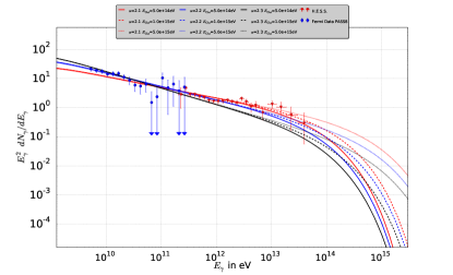
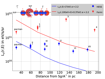
Figure 1: Left: $\gamma$-ray energy spectrum for different source spectral indices and different cut-off energies. Right: $\gamma$-ray luminosity for $\alpha$=2.2 and $E_{\rm cut}=1$ PeV. Blue spheres are observed by H.E.S.S. and re spheres corresponds to Fermi measurements.

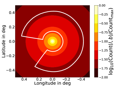
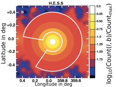
Figure 2: Ratio count map from this work (left) and measured by H.E.S.S. (right)

In order to move away from this semi-analytical approximation toward a full understanding of the PeVatron signature, we further present a new 3D model of both gas and magnetic field distribution in the CMZ.

3 Gas distribution

Concerning the CR propagation, the gas distribution is for two purposes essential as on the one hand, due to inelastic p-p interaction pions are generated which decay among others into $\gamma$-rays. On the other hand, the gas density inside the MCs in the CMZ has enmeshed with the magnetic field strength a consequence of magnetic flux conservation. Wardle and Königl (1990) [11] provide the relation for the MCs near the GC following $\lvert\textbf{B}_{\rm eq}\rvert=1.5\text{ mG}\cdot(\frac{n}{10^{4}\text{ cm}^{-3}})^{{1}/{2}}$. Although Ferrière et al. (2007) [12] presented the average gas density distribution in the CMZ, this model does not include local structures. Therefore, this model will be considered in the diffuse intercloud (IC) medium (ICM) region. The total density profile of the GC region is composed out of three individual components: 1. local MCs whose position, size and density can be taken from Table 1 in [13]; 2. inner 10 pc which is described in [14]; 3. ICM whose analytical description is given in [12] and where the normalization factor is scaled down by the subtraction of the sub-structures to $n_{0,H_{2}}=128.4$ cm^-3 and $n_{0,H}=7.5$ cm^-3. The combined gas density distribution is visualized in Figure 3(a). In the following figures, the red star denotes the position of SgrA*.

4 Magnetic field configuration

There are many models describing the Galactic magnetic field. However, all of them leave out the GC region although a large fraction of the CR flux is supposed to come from there. In order to solve this lack and give a description of the magnetic field in the central 200 pc, we use existing pieces of information. The total magnetic field will be given via a combination of a model for: (1.) the diffuse ICM, (2.) local non-thermal filament (NTF) and (3.) local MC regions. Briefly, the background magnetic field in the ICM and the NTF regions is predominantly poloidal, whereas the horizontal field dominates in the MC regions. Further, an average value of $\overline{B}_{\rm IC}\approx$10 $\mu$G determines the field strength in the ICM [15]. The magnetic field strength in the MC and NTF region can be taken from Table 1 in [13]. The total field in the CMZ is then obtained by a superposition of the magnetic fields which are derived in the next subsections : $\textbf{B}_{\text{tot}}=\textbf{B}_{\text{IC}}^{C}+\sum_{i=1}^{8}\textbf{B}_{\text{NTF,i}}^{C}+\sum_{i=1}^{12}\textbf{B}_{\text{MC,i}}$.

Poloidal field

An analytical divergence-free and isotropic poloidal field model (Model C (FT14-C)) which is taken from [16], will describe the poloidal field in the IC and NTF region.

$$\textbf{B}^{C}=\begin{pmatrix}B_{r}\\ B_{\phi}\\ B_{z}\end{pmatrix}=\begin{pmatrix}\frac{2\,a\,\,z}{(1+a\,z^{2})^{3}}\\ 0\\ \frac{1}{(1+a\,z^{2})^{2}}\end{pmatrix}\cdot B_{1}\cdot e^{-r/L\cdot\frac{1}{(1+a\,z^{2})}}$$

IC region: In the ICM region, the exponential scale length $L=158\text{ pc}/{\ln(2)}=114\text{ pc}$ is adapted to the CMZ geometry following Ferrière et al. (2007) [12] and considering cylindrical geometry. The parameter $a$ governing the opening of field lines away from the z-axis is fitted to the polarization map of Nishiyama et al. (2010) [17] in a region where no NTFs and MCs are located and results in $a=1/(42\ \rm pc)^{2}$. The normalization factor $B_{1}$ is determined by calculating the average value of $\textbf{B}^{C}$ and equating to the observed and expected field strength $\overline{B}$, which yields $B_{1}=\overline{B}_{\rm IC}/{\alpha}\approx 12\,\mu{\rm G}$.

NTF regions:   In the NTF regions, $L$ and $a$ are given by the total longitudinal extend $\Delta l$ and $\Delta b$ of the NTFs following $L=\Delta l/{(2\cdot\ln(2))}$ and $1/{\sqrt{a}}={\Delta b}/{(2\cdot\sqrt{\ln(2)})}$. The value of $\alpha$ corresponding to the normalization factor $B_{1}$ results in all NTFs approximately the same and yields $B_{1}\approx{\overline{B}_{\rm NFT}}/{0.26}\,$.

Horizontal field

As the magnetic field in the dense MCs is predominantly parallel to the Galactic Plane, we will neglect the $B_{z}$ component and regard, therefore, the zonal plane. The relation between the azimuthal component $B_{\phi}$ and radial component $B_{r}$ depends on the characteristics of the MCs, such as the gas density and the intrinsical rotational velocity. The relation in the circumnuclear disc cloud is given in [11] and is also adaptable to other MCs in the GC as all of them exhibits comparable high gas densities and rotational velocities. The resulted ratio $B_{r}/B_{\phi}=\eta$ of each MC is listed in Table 1 in [13] as well. In order to consider the conditions mentioned above in this section, we will derive a suitable field model by considering the Euler’s $\alpha$ and $\beta$ potential. These potentials will deliver a divergence-free expression of the magnetic field following $\vec{B}=\vec{\nabla}\alpha\times\vec{\nabla}\beta=(B_{r},B_{\phi},0)^{T}$ with $\beta=z$ in cylindrical coordinates naturally.

$$\vec{B}=\begin{pmatrix}B_{r}\\ B_{\phi}\\ 0\end{pmatrix}=\begin{pmatrix}\frac{1}{r}\frac{\partial}{\partial{\phi}}\alpha\\ -\frac{\partial}{\partial r}\alpha\\ 0\end{pmatrix}=\begin{pmatrix}\frac{1}{r}\frac{\partial\alpha}{\partial{\psi}}\frac{\partial\psi}{\partial\phi}|_{r}\\ -\frac{\partial\alpha}{\partial{\psi}}\frac{\partial\psi}{\partial r}|_{\phi}\\ 0\end{pmatrix}=\begin{pmatrix}\frac{\rho}{r}\,\xi(\psi)\cdot h(z)\\ -\eta^{-1}\cdot\frac{\rho}{r+b}\,\xi(\psi)\cdot h(z)\\ 0\end{pmatrix}$$ (4)

Here, ${B_{r}}/{B_{\phi}}=\frac{1}{r}\cdot{dr}/{d\phi}|_{\psi,\rho}\overset{!}{=}\eta$ leads to $\psi\approx\phi\pm\eta^{-1}\,\ln\left({r+b}/{\rho+b}\right)$ and we define $\partial\alpha/\partial\psi:=\rho\cdot\xi(\psi)\cdot h(z)$. $\psi$ and $\rho$ denote a reference angle and radius, respectively, and thus $\rho$ will set to the MC radius. $b$ is a free parameter which avoids the singularity of the $\ln$ function at $r=0$ and therefore will set to a negligible fraction of the MC radius. To ensures the physical reality of a magnetic field, i.e., the net magnetic flux is zero, we set $\xi(\psi)=B_{1}\cdot\cos({\psi})$. In doing so, the $h(z)$ is arbitrary, which we set to a Gaussian vertical distribution. The vertical scale length $H_{c}$ is then given by $H_{c}=\rho/\sqrt{2}$. Assembling all relations in Equ. (4) would lead to a singularity due to the factor $\propto 1/r$. In the physical context, here, all field lines meet at $r=0$ due to this expression. We prevent the singularity within a small radius $r^{\prime}$ which should correspond to a negligible fraction of the MC radius, by introducing a new $\phi$ component. The additional $\phi$ component connects two field lines instead of allowing them to meet each other. Then, the magnetic field in a MC is given by Equ. (5)

$$\vec{B}^{r>r^{\prime}}_{\text{MC}}=\beta\begin{pmatrix}\frac{R}{r}\\ \mp\eta^{-1}\frac{R}{r+b}\\ 0\end{pmatrix}\text{ with }v(r)=\frac{1}{\eta}\cdot\ln\left(\frac{r+b}{R+b}\right),\beta=B_{1}\cos\left(\pm v(r)+m{\phi}\right)\cdot\exp\left(-\frac{z^{2}}{H_{c}^{2}}\right)$$

$$\vec{B}^{r<r^{\prime}}_{\text{MC}}=\beta\cdot\frac{R}{r^{\prime}}\left(\frac{3r}{r^{\prime}}-\frac{2r^{2}}{r^{\prime 2}}\right)\begin{pmatrix}1\\ \mp\frac{r}{\eta(r+b)}\left(1+\frac{6(r-r^{\prime})}{2\,r-3\,r^{\prime}}\left(\frac{\sin(\pm v(r)+m\phi)-\sin(\pm v(r))}{\cos(\pm v(r)+m\phi)}\right)\right)\\ 0\end{pmatrix}.$$ (5)

For more Details on the magnetic field modeling in the GC, see [13] (submitted).

5 Results

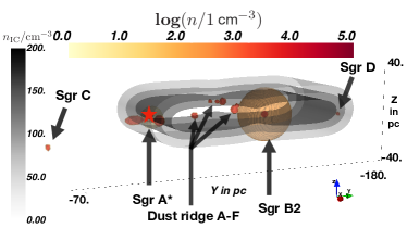
(a) Combined gas density of the CMZ region: the diffuse ICM is shown as gray contours and the contour represents a density level.

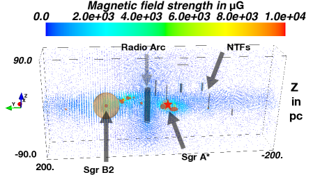
(b) The total magnetic field strength in the CMZ is given in $\mu$G. Additionally, NTFs a visualized by black cylinders.

Figure 3(b) displays the 3D configuration and strength of the total magnetic field in the CMZ. The polarization map of this total field and the measurements in the CMZ by [17] are shown in Figure 3 in order to cross-check the results. In total, the most relevant structures in the region $|l|<1.35\degree$ and $|b|<0.6\degree$ are well described by the model derived in this work. Thus, regions with good conformity, e.g., $|b|<0.3\degree$ indicate a dominant regular magnetic field.

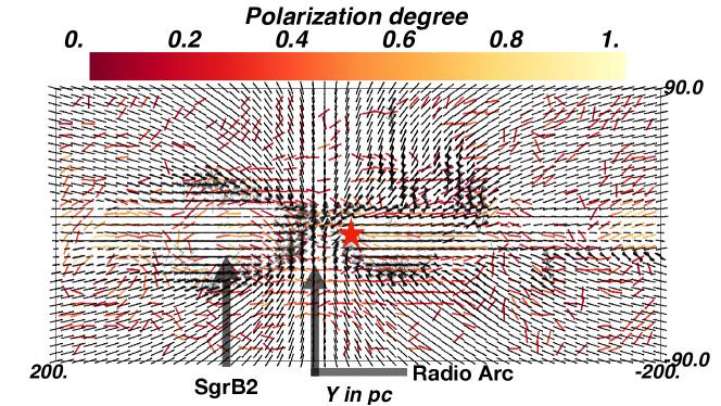
Figure 3: Magnetic field configuration as derived in this work is visualized by black dashed lines and as measured by [17] by colored dashed lines. Blurred black configurations indicate polarization degree with respect to the $x$ direction.

Impact on cosmic ray propagation

In order to test our magnetic field model on CR propagation, we consult the CR propagation tool CRPropa 3.1 [18]. Skipping all technical detail, we present the result of the model build in this work (GBFD19) and the standard field used in cosmic-ray propagation presented in Jansson and Farrar (2012) [3] (abbreviated as JF12 in the following). By using the mulit-particle picture of CRPropa tool, we construct an $234\times 234\times 234$ pc³ environment, inject $10^{5}$ particles at energies 1 TeV- 1000 TeV in center and detect each particle after a discrete time step of $\Delta t_{i}=1$ pc/c for 234 times. As a first result, at a distance $Y=\pm 100$ pc and $Z=0$ pc, the JF12 configuration results in a flux level close to zero particles, whereas the GBFD19 field reaches a level of $10^{3}$ protons. The entrapping ability of the GBFD19 could explain the longitudinal extension up to 220 pc of the diffuse $\gamma$-ray emission detected by H.E.S.S..

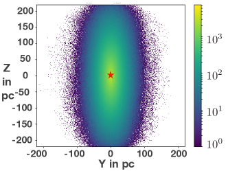
Figure 4: Protons propagated in the GBFD19 (left) and in the JF12 (right) field between $1-1000$ TeV.

6 Summary and conclusion

In the first part of this work, we consider approximated ambient conditions of the GC in the transport equation (1). Hereafter, we present the solution and calculate the diffuse $\gamma$-ray emission as described in Abramowski et al. (2016) [1]. Furthermore, we calculate the radial distribution of the $\gamma$-ray luminosity and compare with the data presented in Gaggero et al. (2017) [2] and Abramowski et al. (2016) [1]. We assert that under our assumptions, the injection of a centralized source is not able to explain the diffuse $\gamma$-ray emission at higher longitudes. Therefore, we are aimed at modeling an accurate 3D gas and magnetic field distribution. For the former modeling, we combined a 3 component model made by a diffuse ICM, local MC and by the inner 10 pc around SgrA*. The magnetic field is separated into 3 regions: 1. IC 2. NTF 3. MC region where the first 2 regions are described by a poloidal field model which is taken from [16]. The latter region is described by a horizontal model which is exclusively derived and describe each MC individually by considering the ambient conditions such as the gas density and intrinsic rotational velocity. The total magnetic field is then given by a superposition of the magnetic field of each region. The polarization map result is in a strong agreement with the data measured by [17]. The influence of this field on CR propagation exhibits a significant impact. In fact, the field structure in the CMZ produce an entrapment of CR in longitudinal direction and therefore is most likely responsible for the longitudinal extension up to 220 pc of the diffuse $\gamma$-ray emission detected by H.E.S.S.. However, for a quite validation further simulation of the production $\gamma$-ray in an realistic environment has to be performed. The 3D gas and magnetic field distribution presented in this work makes this goal more accessible to the GC investigators.

References

- [1] A. Abramowski et al. Acceleration of petaelectronvolt protons in the Galactic Centre. Nature, 531:476, 2016.
- [2] D. Gaggero, D. Grasso, A. Marinelli, M. Taoso, and A. Urbano. Diffuse cosmic rays shining in the Galactic center: A novel interpretation of H.E.S.S. and Fermi-LAT -ray data. Phys. Rev. Lett., 119(3):031101, 2017.
- [3] Ronnie Jansson and Glennys R. Farrar. A new model of the galactic magnetic field. The Astrophysical Journal, 757(1):14, 2012.
- [4] S. Krakau and R. Schlickeiser. Pion Production Momentum Loss of Cosmic Ray Hadrons. The Astrophysical Journal, 802:114, 2015.
- [5] Rolf Gusten and Sabine D. Philipp. Galactic Center molecular clouds. Springer Proc. Phys., 91:253–264, 2004.
- [6] Masato Tsuboi, Toshihiro Handa, and Nobuharu Ukita. Dense molecular clouds in the galactic center region. i. observations and data. The Astrophysical Journal Supplement Series, 120(1):1, 1999.
- [7] L. Jouvin, R. Terrier, and A. Lemiere. Origin of the VHE cosmic rays excess in the Galactic Center. In 41st COSPAR Scientific Assembly, volume 41 of COSPAR Meeting, July 2016.
- [8] Mehmet Guenduez, Julia Becker Tjus, Björn Eichmann, and Francis Halzen. Cosmic ray cradles in the galaxy. In Zbigniew Szadkowski, editor, Cosmic Rays, chapter 6. IntechOpen, Rijeka, 2018.
- [9] S. R. Kelner, F. A. Aharonian, V. V. Bugayov. Energy spectra of gamma-rays, electrons and neutrinos produced at proton-proton interactions in the very high energy regime. Physical Review D, 74:034018, 2006.
- [10] S. Gillessen, R. Genzel, T. K. Fritz, E. Quataert, C. Alig, A. Burkert, J. Cuadra, F. Eisenhauer, O. Pfuhl, K. Dodds-Eden, C. F. Gammie, and T. Ott. A gas cloud on its way towards the supermassive black hole at the Galactic Centre. 481(7379):51–54, 2012.
- [11] M. Wardle and A. Königl. A model for the magnetic field in the molecular disk at the Galactic center. The Astrophysical Journal, 362:120–134, October 1990.
- [12] Katia Ferrière, William Gillard, and Pierre Jean. Spatial distribution of interstellar gas in the innermost 3 kpc of our Galaxy. Astron. Astrophys., 467:611–627, 2007.
- [13] Mehmet Guenduez, Julia Becker Tjus, Katia Ferrière, and Ralf-Jürgen Dettmar. A novel analytical model of the magnetic field configuration in the Galactic Center. arXiv e-prints, 2019.
- [14] K. Ferrière. Interstellar gas within ~10 pc of Sagittarius A*. Astron. & Astroph., 540:A50, April 2012.
- [15] K. Ferrière. Interstellar magnetic fields in the Galactic center region. Astron. & Astroph., 505:1183–1198, October 2009.
- [16] K. Ferrière and P. Terral. Analytical models of X-shape magnetic fields in galactic halos. Astron. & Astroph., 561:A100, January 2014.
- [17] Shogo Nishiyama, Hirofumi Hatano, Motohide Tamura, Noriyuki Matsunaga, Tatsuhito Yoshikawa, Takuya Suenaga, James H. Hough, Koji Sugitani, Takahiro Nagayama, Daisuke Kato, and Tetsuya Nagata. Magnetic field configuration at the galactic center investigated by wide-field near-infrared polarimetry: Transition from a toroidal to a poloidal magnetic field. The Astrophysical Journal Letters, 722(1):L23, 2010.
- [18] Lukas Merten, Julia Becker Tjus, Horst Fichtner, Bj Eichmann, and G. Sigl. CRPropa 3.1 a low energy extension based on stochastic differential equations. JCAP, 1706(06):046, 2017.