Optimal Detection of Rotations about Unknown Axes by Coherent and Anticoherent States
Abstract
Coherent and anticoherent states of spin systems up to spin are known to be optimal in order to detect rotations by a known angle but unknown rotation axis. These optimal quantum rotosensors are characterized by minimal fidelity, given by the overlap of a state before and after a rotation, averaged over all directions in space. We calculate a closed-form expression for the average fidelity in terms of anticoherent measures, valid for arbitrary values of the quantum number . We identify optimal rotosensors (i) for arbitrary rotation angles in the case of spin quantum numbers up to and (ii) for small rotation angles in the case of spin quantum numbers up to . The closed-form expression we derive allows us to explain the central role of anticoherence measures in the problem of optimal detection of rotation angles for arbitrary values of .
1 Introduction and main result
Historically, advances in measurement techniques often are the reason for physics to progress. Over time, metrology has developed as a subject of its own, especially in the context of defining standard units of measurement for physical quantities.
Quantum theory provides new perspectives on measurements, ranging from fundamental limitations on measurements [1], new opportunities [2] as well as technical challenges and even philosophical quagmires [3]. From a practical point of view, quantum information science requires ever better control of microscopic systems and, hence, measurements which are as accurate as possible. More specifically, quantum metrology [4] aims at finding bounds on the achievable measurement precision and at identifying states which would be optimal for quantum measurements or other specific tasks. The optimal transmission of a Cartesian frame [5] or the efficient detection of inhomogeneous magnetic fields [6] are typical examples. While the classical Cramér-Rao theorem [7, 8] provides a lower bound on the variance of random estimators by means of the Fisher information, its quantum-mechanical counterpart provides bounds for quantum parameter estimation theory [9]. The quantum Cramér-Rao bound is expressed as the inverse of the quantum Fisher information, which can be geometrically interpreted as the (Bures) distance between two quantum states differing by an infinitesimal amount in their parameter [10, 11]. It provides lower bounds on the variance of any quantum operator whose measurement aims at estimating the parameter. Optimal measurement is achieved by maximizing the quantum Fisher information over parameter-dependent states.
The quantum Cramér-Rao bound was calculated for instance in the reference frame alignment problem [12]. This problem involves estimating rotations about unknown axes. It has been shown in [13] that spin states with vanishing spin expectation value and isotropic variances of the spin components are valuable for estimating such rotations, as they saturate the quantum Cramér-Rao bound for any axis. Also, recently, the problem of characterizing a rotation about an unknown direction encoded into a spin- state has been considered in [14].
In this paper, we are interested to determine whether a quantum system has undergone a rotation by a known angle about an unknown axis . Suppose first that we apply the rotation by to an initial state about a known axis and perform a measurement of the projector in the rotated state . The expectation value of the observable is given by
| (1) |
i.e. by the fidelity between the initial state and the final state. The fidelity equals the probability to find the quantum system in the initial state after the rotation. Thus, the probability to detect that the rotation has occurred is given by the quantity . Therefore, the measurement will be most sensitive if the rotation is applied to states which minimize the expression (1) for given angle and rotation axis.
Next, suppose that only the rotation angle is well-defined while the rotation axis is not known, as described in [15]. This situation occurs, for example, when spins prepared in the state are—during the measurement sequence—subjected to a magnetic field whose direction randomly fluctuates on a time scale much larger than the Larmor period. Measuring the observable on an ensemble of identically prepared systems will now produce a value of the fidelity (1) averaged over all possible spatial directions . Then, the most suitable quantum states —called optimal quantum rotosensors in [15]—are determined by the requirement that the average fidelity
| (2) |
achieve its minimum, for a given value of the parameter .
The fidelity (1) and its average (2) also play a role when setting up experiments which aim to determine an unknown rotation angle as accurately as possible. This is explained in more detail in Appendix A.
For the spin values , optimal quantum rotosensors have been identified [15], using an approach which combines analytical and numerical methods. For rotation angles close to , the average fidelity is minimized systematically by coherent spin states. Coherent spin states are strongly localized in phase space and entirely specified by a spatial direction into which they point on the Bloch sphere [16]. For small rotation angles , the average fidelity is minimized by anticoherent states, which are characterized by the fact that they do not manifest any privileged direction; in this respect, they are as distinct as possible from coherent states [17]. The role of anticoherent states for optimal detection of rotations has also been observed and was subsequently quantified in terms of quantum Fisher information in [13]. Between these two extreme cases of and , optimal states are neither coherent nor anticoherent in general. From an experimental point of view, anticoherent and other non-classical spin states have been created using a variety of physical systems. For instance, anticoherent states of quantum light fields have been generated using orbital angular momentum states of single photons with their usefulness for quantum metrology being established in [18]. Non-classical spin states—including Schrödinger cat states (c.f. Sec. 4)—of highly magnetic dysprosium atoms with spin quantum number have been created in order to enhance the precision of a magnetometer [19].
The main result of the present paper is a closed-form expression of the average fidelity , valid for arbitrary values of . A rather general argument, based solely on the symmetries of the average fidelity , shows that it must be a linear combination of the form
| (3) |
as explained in detail in Sec. 2. In this expression, the are the anticoherence measures of a state , introduced in [20] and given explicitly in Eq. (10), while the real-valued functions are trigonometric polynomials independent of , and is the largest integer smaller than or equal to . The main challenge is to calculate the -dependent coefficients , which we do in Sec. 3.
In earlier works, the average fidelity had been expressed as a sum of functions of weighted by state-dependent coefficients, upon representing the state in the polarization-tensor basis [15]. The advantage of relation (3) is that the average fidelity depends on the state under consideration only through its measures of anticoherence, and thus it directly relates to the degree of coherence or anticoherence of the state. Expression (3) allows us to identify optimal quantum rotosensors for spin quantum numbers up to thereby confirming the role played by coherent and anticoherent states beyond . Readers mainly interested in the optimal quantum rotosensors may want to directly consult Sec. 4.
Let us outline the overall argument leading to the expression of the average fidelity in (3). In Sec. 2, we introduce a number of tools and concepts feeding into the derivation of (3): first, we discuss the symmetries built into the average fidelity , followed by a brief summary of the Majorana representation which enables us to interpret spin- states as completely symmetric states of qubits. This perspective allows us to introduce, for , the anticoherence measure , defined as the linear entropy of the -qubit reduced density matrix of . To actually carry out the integration in Eq. (2), we will use a tensor representation (see Sec. 2.5) of mixed spin- states generalizing the Bloch representation. In addition, this representation also enables us to exploit the symmetries of the average fidelity which can only depend on expressions invariant under rotations. As shown in Sec. 2.6, it is then possible to establish a linear relation between these invariants and the anticoherence measures , which finally leads to (3).
Section 3 is dedicated to deriving explicit expressions for the functions . This will be done in two ways: the first one is based on the fact that anticoherence measures are explicitly known for certain states, so that the functions appear as solutions of a linear system of equations. The second approach makes use of representations of the Lorentz group and allows us to obtain a general closed expression. In Sec. 4 we make use of this closed-form expression to identify the optimal quantum rotosensors. We conclude with a brief summary given in Sec. 5.
2 Concepts and tools
In this section, we introduce the tools that will be needed to address the optimality problem described in the Introduction.
2.1 Notation
Quantum systems with integer or half-integer spin are described by states of the Hilbert space with , which carries a -dimensional representation of the group SU. The components of the angular momentum operator satisfy , , where is the Levi-Civita symbol. Denoting unit vectors in by
| (4) |
the operator
| (5) |
describes a rotation by an angle about the direction .
2.2 Symmetries
By definition, the average fidelity in (2) is a positive function of the angle and of the state and possesses three symmetries: it is -periodic in , symmetric about , and invariant under rotation of .
Periodicity with period comes from the fact that . Symmetry about is equivalent to
| (6) |
which can be shown using and the fact that the set of directions averaged over in (2) is the same irrespective of the sign of the unit vector since the fidelity (1) is given by the the squared modulus of the overlap between the states and .
Invariance under rotation of can be understood in the following way. Let be a unitary operator representing a rotation in by an angle about the direction , acting on a state . Then the average fidelities associated with the states and are equal. Indeed, we have
| (7) |
and
| (8) |
with the vector obtained by the rotation SO associated with . Due to the invariance under rotations of the unit-ball region appearing in (2) (invariance of the Haar measure used), the result of the integration will be the same, leading to
| (9) |
This invariance of the fidelity can be seen in a geometrically appealing way by use of the Majorana representation, which we consider now.
2.3 Majorana representation of pure spin states
The Majorana representation establishes a one-to-one correspondence between spin- states and -qubit states that are invariant under permutation of their constituent qubits (see e.g. [21, 22, 23]). It allows to geometrically visualise a pure spin- state as points on the unit sphere associated with the Bloch vectors of the qubits. The Majorana points are often referred to as stars, and the whole set of Majorana points of a given state as its Majorana constellation. Considering a spin- state as an -qubit state, any local unitary (LU) operation with transforms into a state whose Majorana constellation is obtained by the constellation of rotated by the SO rotation associated with . Spin-coherent states take a very simple form in the Majorana representation, as they can be seen as the tensor product of some spin- state . Their constellation thus reduces to an -fold degenerate point.
The fidelity (1) is given by the squared modulus of the overlap between and . Since the Majorana constellation of is obtained by rigidly rotating that of , the fidelity (1) only depends on the relative positions of these two sets of points. The average transition probability is obtained by integrating over all possible constellations obtained by rigid rotations of the Majorana constellation of , and therefore it must be invariant under LU. In other words, the equality (9) takes the form .
2.4 Anticoherence measures
An order- anticoherent state is defined by the property that is independent of the vector for all . In the Majorana representation, it is characterized by the fact that its -qubit reduced density matrix is the maximally mixed state in the symmetric sector [24].
The degree of coherence or -anticoherence of a spin- pure state can be measured by the quantities , which are positive-valued functions of [20]. Let be the -qubit reduced density matrix of the state interpreted as a -qubit symmetric state with ; it is obtained by taking the partial trace over all but qubits (it does not matter which qubits are traced over since is a symmetric state). The measures are defined as the rescaled linear entropies
| (10) |
where is the purity of . Thus, anticoherence measures are quartic in the state and range from to , and are invariant under SU rotations. Spin-coherent states are characterized by pure reduced states and thus are the only states such that . Anticoherent states to order are characterized by and thus are the only states such that . In particular, if a state is anticoherent to some order , then it is necessarily anticoherent to all lower orders since reductions of the maximally mixed state are maximally mixed.
While for any state we have , not all possible tuples are realised by a physical state . For instance, since implies that for all , the choice and cannot correspond to any state. We denote the domain of admissible values of the measures by .
2.5 Tensor representation of mixed states
We now introduce a tensor representation of an arbitrary (possibly mixed) spin- state acting on a -dimensional Hilbert space with , following [24]. Any state can be expanded as
| (11) |
Here and in what follows, we use Einstein summation convention for repeated indices, with Greek indices running from to and Latin indices running from to . Here, the are Hermitian matrices invariant under permutation of the indices.
The are real coefficients also invariant under permutation of their indices, which enjoy what we call the tracelessness property
| (12) |
Whenever has some indices equal to , we take the liberty to omit them, so that e.g. for a spin- state may be written (recall that the order of the indices does not matter). In the case of a spin-coherent state given by its unit Bloch vector , the coefficients in (11) are simply given by , with .
In the following, we will make use of two essential properties of the tensor representation. Namely, let us consider a state with coordinates in the expansion (11). Then, the tensor coordinates of the -qubit reduced state in the expansion (11) are simply given by . Thus, since we omit the zeros in the string , the tensor coordinates of and coincide for any string of nonzero indices.
The second property we use is that for states and in the form (11) with tensor coordinates respectively and we have
| (13) |
Note that this equality holds despite the fact that the are not orthogonal; this property follows from the fact that these matrices form a -tight frame, see [24]. In particular, for a pure state , the equality translates into
| (14) |
while the purity of the reduced density matrix reads
| (15) |
The normalization condition imposes . A consequence of (12) is then that .
2.6 SU-Invariants
If SU(2) and SO(3) is the corresponding rotation matrix, then the tensor coordinates of with are the where is the orthogonal matrix
| (16) |
That is, transforms as a tensor. Under such transformations, goes into , where the last equality comes from orthogonality of . Thus is an SU(2) invariant. Similarly, and, more generally, any product of the such that all indices are contracted (i.e. summed from to ), are invariant under SU(2) action on . One can then show by induction that products of terms with where all indices appear in pairs and are summed from to are also SU(2) invariant. For instance, , , , are such invariants.
Invariants of degree 1 in are of the form , where the appear in pairs. Since the order of indices is not relevant, these invariants are in fact of the form . Because of Eq. (12), each pair can be replaced by zeros in the string, so that . Therefore, there is no invariant of degree 1. The invariants of degree 2 are products of the form where indices appear in pairs and are summed from to . If the two indices of a pair appear in the same index string ( or ), then from Eq. (12), they can again be replaced by zeros and discarded. Thus the invariants of degree 2 are , , and more generally, for ,
| (17) |
Using (10) and (15) one can express the invariants in terms of a linear combination of the . Indeed, grouping together terms with the same number of nonzero indices in (15) yields
| (18) |
Inverting that relation via the binomial inversion formula, we obtain
| (19) |
and by use of (10) we finally can express the -invariants in terms of anticoherence measures,
| (20) |
for .
2.7 General form of the average fidelity
Let us now explain why the average fidelity given in Eq. (3) is a linear combination of the lowest anticoherent measures . Due to its rotational symmetry, the average fidelity —when considered as a function of the tensor coordinates —can only involve invariants constructed from these coordinates. With being quadratic in , it must also be quadratic in . As there is no invariant of degree 1, the only invariants that can appear in the expression of are the invariants defined in (17). Since the quantity is quadratic it must be a linear combination of the coefficients which, according to Eq. (20), implies that is also a linear combination of the . Furthermore, the identity
| (21) |
which holds for any pure state, means that the anticoherence measures for can be expressed in terms of the measures for . Therefore, (3) is the most general form the fidelity can take, with the dependence in being only in the coefficients of the measures .
2.8 Generalizations
It is worth stressing that the form (3) for the average fidelity also holds for more general types of average fidelity
| (22) |
between a state and its image under the unitary
| (23) |
where is an arbitrary real analytic function, ensuring that is an Hermitian operator. Indeed, from an argument similar to that of Sec. 2.6, the generalized fidelity (22) can be expressed as a function of the and hence of the . An interesting case is when is a spin-squeezing operator, which corresponds to choosing . Moreover, if we now consider the quantities
| (24) |
with integer , the same arguments show that they are linear combinations of higher-order invariants, leading to generalizations of the relation (20).
3 Closed form of the average fidelity
In this section we derive the angular functions , which characterize the fidelity through (3), in two different ways. The first method (subsection 3.1) is based on the fact that anticoherence measures can be evaluated explicitly for Dicke states. The second method (subsection 3.2) exploits a tensor representation of spin states [24] which uses Feynman rules from relativistic spin theory. These approaches are independent and we checked, for all integers and half-integers up to , that as expected they yield the same angular functions. Technical detail is delegated to appendices in both cases.
3.1 Derivation based on anticoherence measures for Dicke states
In the following, we will work in the standard angular momentum basis of , for positive integer or half-integer value of . It consists of the Dicke states given by the common eigenstates of , the square of the angular momentum operator , and of its -component . In this basis, any spin- state can be expanded as
| (25) |
with and .
The first derivation is based on the fact that both the measures of -anticoherence and the average fidelities can be determined explicitly for Dicke states. Their measures of -anticoherence are given by
| (26) |
They can readily be obtained from the purities for a state of the form (25), which were calculated in [20] in terms of the coefficients and read
| (27) |
with
| (28) |
As for the fidelity, the calculation is done in Appendix B and yields
| (29) |
with Clebsch-Gordan coefficients and the functions defined in Eqs. (77)–(78). The angular functions are then solutions of the system of linear equations
| (30) |
This system can easily be solved for the lowest values of . A general (but formal) solution can then be obtained by inverting the system (30).
3.2 Derivation based on relativistic Feynman rules and tensor representation of spin states
The second approach allows us to derive a closed-form expression for the functions . It is based on an expansion of the operator
| (31) |
with and , as a multivariate polynomial in the variables . This operator is a -dimensional representation (with ) of a Lorentz boost in the direction of the 4-vector . As shown in [25], it can be written as
| (32) |
The identification of Eqs. (31) and (32) defines the matrices appearing in (11) (see [24] for detail). Taking
| (33) |
in (31), we see that reduces to a rotation operator,
| (34) |
with
| (35) |
Moreover, for a state given by (11) we have
| (36) |
according to Eq. (24) of [24], which holds for any 4-vector . Thus, with , using the identity (34) and the expansion (32) for the rotation operator in (1) allows us to explicitly perform the integral in Eq. (2), resulting in
| (37) | ||||
where denotes complex conjugation (which acts on only because of the choice (33) and using ). Each term with indices equal to 0 is proportional to
| (38) |
For the remaining nonzero indices, we have from (33) that , so that (37) involves an integral of the form
| (39) |
These integrals are performed in Appendix C. The integrals (39) are in fact precisely given by the tensor coordinates of the maximally mixed state, whose expression is explicitly known. One can therefore rewrite (37) as
| (40) | ||||
where the sum over runs over all strings of indices (between 0 and 3) containing zeros. An explicit expression for this sum is derived in Appendix C, leading to the compact expression
| (41) |
with numbers
| (42) |
Note that the sum over in (41) can start at because the factor in implies that for . Using the symmetry we may rewrite (41) as
| (43) | ||||
From (10) we obtain a relation between and , namely , which yields the explicit expression of the polynomials in Eq. (3) as
| (44) |
with coefficients
| (45) |
Note that although and are not well-defined for , the ratio in (38) always is, so that the expression above is valid over the whole range of values of . For spin-coherent states, all vanish and thus from Eq. (3), which coincides with the expression obtained in [15]. For the smallest values of , we recover the functions obtained in Section 3.1. In the following section, we will use the functions given in (44) to identify optimal quantum rotosensors.
4 Optimal quantum rotosensors
4.1 Preliminary remarks
We now address the question of finding the states which minimize the average fidelity for fixed rotation angles . According to Eq. (3), the fidelity is a linear function of the anticoherence measures with . Linearity, when combined with the fact that the domain , over which the measures vary, is bounded implies that the fidelity must attain its minimum on the boundary. The minimization problem thus amounts to characterizing this domain . Unfortunately, even for the smallest values of , no simple descriptions of this domain are known.
We will first determine the states minimizing the -periodic average fidelity for values of up to , with the rotation angle taking values in the interval (which is sufficient due to the symmetry (6)). Then we will examine the limiting case of angles close to for arbitrary values of the quantum number . Throughout this section, we will expand arbitrary states with spin in terms of the Dicke states, as shown in Eq. (25).
For spins up to the states minimizing the average fidelity are known [15]. In Sec. 4.2, we show that our approach based on the expression (3) correctly reproduces these results. Then, in Sec. 4.3, we consider the minimization problem for spin quantum numbers up to , mainly identifying the optimal rotosensors within various ranges of the rotation angle by numerical techniques. More specifically, for a fixed angle , is a function of the which can be parametrized by the complex coefficients entering the expansion (25) of the state in the Dicke basis (see Eq. (27)). We search numerically for the minimum value of with respect to the , taking into account the normalization condition . In most cases this numerical search converges towards states which have simple analytic expressions which are the ones that we give. For each value of , we performed this search at about 1000 evenly spaced values of in order to explore the whole range of rotation angles. Whenever we find a region of values of in which is the optimal state adjacent to a region where is optimal, at the critical angle separating these two regions, one should have because the average fidelity is a continuous function of . Therefore, the critical angle is a solution of the equation
| (46) |
4.2 Rotosensors for arbitrary rotation angles and
4.2.1
For a spin , all pure states are coherent: each state can be obtained by a suitable rotation of the state . Since the fidelity is invariant under rotation, all states are equally sensitive to detect rotations for any angle .
4.2.2
For , the expansion (3) takes the form
| (47) |
with
| (48) | ||||
The first strictly positive zero of is given by . In the interval , where is negative, the fidelity is minimized by states with , i.e. by -anticoherent states. For , the fidelity takes the same value for all states , namely . For rotation angles in the the remaining interval, , where is positive, is minimized for states with , i.e. coherent states. Thus, we indeed recover the results obtained in [15].
4.2.3
In this case, the average fidelity (3) reads
| (49) |
with
| (50) | ||||
The situation is basically the same as for . The first strictly positive zero of the coefficient is found to be . Hence, in the interval where is negative, the fidelity is minimal for -anticoherent states. At the value , the fidelity takes the same value for all states , namely, . Otherwise, is minimized for coherent states, thereby reproducing earlier results [15].
4.2.4
For , the fidelity (3) is a linear combination of three terms,
| (51) |
with the angular functions , displayed in Appendix D. They all take negative values in the interval , with the first strictly positive zero of . The tetrahedron state
| (52) |
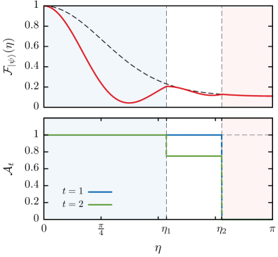
whose Majorana points lie at the vertices of a regular tetrahedron, is -anticoherent, and for it is the only state (up to LU) with [26]; hence it provides the optimal rotosensor for angles in the interval . For larger angles of rotation comprised between and , we find numerically that an optimal state is the Schrödinger cat state
| (53) |
which is only 1-anticoherent, with and . For values , the optimal state is a coherent state.
We thus obtain numerically three intervals with three distinct optimal states corresponding to , and , respectively. In order to find the critical angles, we solve Eq. (46). The angle separating the first two regions is a solution of . The first positive zero of is , which coincides with the numerically obtained value. The angle at which the second and third region touch, is a zero of . Its first strictly positive zero is given by
| (54) |
with and , and we have indeed . The results we obtained are summarized in Fig. 1; they agree with the findings of [15].
It is noteworthy that the state (53) is not the only state with anticoherence measures and . For instance, any state of the form
| (55) |
with and come with the same measures of anticoherence, as readily follows from Eq. (27). These states are thus also optimal in the interval , thereby removing the uniqueness of optimal rotosensors observed for and .
4.3 Rotosensors for
4.3.1
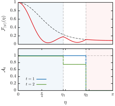
For , there is no anticoherent state of order but only of order [12]. Numerical optimization shows that the optimal state for small angles of rotation is the -anticoherent state with the largest measure of -anticoherence, that is given by
| (56) |
and has and . This state is found to be optimal up to a critical angle , which is obtained from Eq. (46) and coincides with the first strictly positive zero of . It is worth noting that the optimal state (56) was also found to be the most non-classical spin state for , both in the sense that it maximizes the quantumness [27] and that it minimizes the cumulative multipole distribution [28, 29]. The Majorana constellation of this state defines a triangular bipyramid, which is a spherical -design [30, 31], thus corresponding to the arrangement of point charges on the surface of a sphere which minimize the Coulomb electrostatic potential energy (solution to Thomson’s problem for 5 point charges, see [32]).
For larger angles of rotation ranging between and , we find that an optimal state is
| (57) |
unlike in the case , we found this state for to be the only state (up to LU) with and . For , we find that coherent states are optimal. The transition occurs at the first strictly positive zero of . Our results are summarized in Fig. 2.
4.3.2
Anticoherent states of order do exist for . They are all connected by rotation to the octahedron state
| (58) |
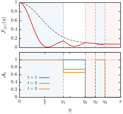
whose Majorana points lie at the vertices of a regular octahedron. Therefore, the state (58) is, at small , the unique optimal quantum rotosensor (up to LU) for . Numerical optimization shows that the octahedron state is optimal up to a critical angle coinciding with the first strictly positive zero of , and that, for larger angles, the state
| (59) |
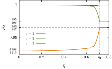
with , and is optimal up to a critical angle coinciding with the first strictly positive zero of . We found that this is the only spin- state (up to LU) with , and . Coherent states are found to be optimal for angles of rotation in the ranges and with and coinciding with the second and third strictly positive zeros of . In the range , the octahedron state (58) becomes again optimal (although the three functions for are not simultaneously negative in that range). Our results are displayed in Fig. 3.
4.3.3
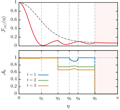
This is the smallest spin quantum number for which a smooth variation of the optimal state with is observed, resulting in the complex behaviour displayed in Figs. 4 and 5. There are no anticoherent states to order for , but there exist anticoherent states to order . The optimal state for small angles of rotation (by which we mean here ) turns out to be one of those. Numerical optimization yields the state
| (60) |
with measures of anticoherence and . This is not the state with the highest measure of -anticoherence, as the state
| (61) |
has measures of anticoherence , and . The latter state is found to be optimal for with (not identified) and coinciding with the first strictly positive zero of . The state
| (62) |
with , and is found to be optimal for and with and coinciding with the third and fourth strictly positive zeros of and with the first strictly positive zero of . In the interval , coherent states are found to be optimal.
4.4 Rotosensors for small rotation angles and arbitrary values of
4.4.1 Angular functions at small angles
According to Secs. 4.2 and 4.3 optimal rotosensors for integer values of spin () are given by -anticoherent states while for half-integer spin () the fidelity is optimized by states which are anticoherent of order , respectively, and possess large anticoherence measures for values of up to . This fact can be understood quite generally through the behaviour of the functions at small for arbitrary values of . In the vicinity of , the functions given in Eq. (44) take the form
| (63) |
with coefficients given by Eq. (45). These coefficients are strictly negative for all and all , since and is either for or positive for . This implies that all functions are negative in some interval around . Thus, the fidelity is a linear combination of the with negative coefficients in that interval. Since , it follows that if there exists a state with for all —that is, an anticoherent state to order —then this state provides an optimal quantum rotosensor for in that interval.
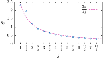
This interval can be made more specific, at least for the lowest values of . Let denote the first zero of . Numerical results up to indicate that all functions for are negative for , so that an anticoherent state to order (if it exists) is optimal in the whole interval . As shown in Fig. 6, is found to scale as for large . A simple explanation for this is that the expansion of the function as is dominated by the term (note however that is even better approximated by ). Conversely, the states maximizing for small angles of rotation are the states with for all , i.e. coherent states.
To see whether any general pattern emerges, we now identify optimal small-angle rotosensors for the next few values of the spin quantum numbers.
4.4.2
For , there is no anticoherent state to order . We find that the optimal state for small angles of rotation is the -anticoherent state
| (64) |
with and .
4.4.3
For , there is no anticoherent state to order . The anticoherent states of order with the largest are found to be of the form
| (65) |
with . Their measures of anticoherence are , and . Among these states, the one with has the largest value of and numerical results suggest that this is the optimal state for small angles of rotation.
4.4.4
For , there is no anticoherent state to order . We find that the optimal state for small angles is the -anticoherent state
| (66) |
with , and .
| Interval | |||
|---|---|---|---|
4.4.5 Arbitrary values of
As was mentioned earlier, if an anticoherent state to order exists for a given , then this state gives rise to an optimal quantum rotosensor for . This applies to values and , which are the only cases where existence of anticoherent states to order has been established (see e.g. [33, 20]).
The situation is less straightforward if such a state is not known to exist from the outset. The only general conclusion one can draw is that minimizing the average fidelity for a fixed angle corresponds to maximizing the measures within the domain (by definition, is the set of all reachable so that by changing , we will remain within ). In this sense, the more anticoherent a state is, the more sensitive it will be as a quantum rotosensor. In general, varying will change all anticoherence measures simultaneously. The challenge is to determine whether a state with given values of the measures exists and, if it does, to identify it.
The maximal order of anticoherence that a spin- state can display is generally much smaller than , typically for large spins [33]. Numerical results for seem to suggest that the pairs for which a -anticoherent spin- state exists coincide with those for which a -points spherical -design exists in three dimensions [34]. The latter have been tabulated up to [31]. For example, the first pairs for are given by , , , , , , .
5 Summary and conclusions
The main result of this work is a closed-form expression (3) for the fidelity between a state and its image under a rotation by an angle about an axis , averaged over all rotation axes. The expression takes the form of a linear combination of anticoherence measures , with explicit -dependent coefficients. It follows that not only spin- states which are related by a global rotation of the axes come with the same average fidelity, but more generally all states with identical purities of their reduced density matrices (calculated for any subset of their constituent spin- in the Majorana representation). This gives an explanation for the observation of [15] that optimal states are not necessarily unique. Moreover, since the fidelity is linear in the anticoherence measures, optimal states correspond to values of on the boundary of the domain of admissible values. This shows the relevance of characterizing the domain .
The expression (3) allows us to characterize states which optimally detect rotations by their degree of coherence or anticoherence. At small angles , where the coefficients of the measures are all negative, optimality of detection of rotations goes hand in hand with high degrees of anticoherence. For angles close to , however, numerical results support the claim that optimality is achieved throughout by spin coherent states.
We also performed a systematic investigation of states minimizing the average fidelity for small values of , for all integers and half-integers from to . Table 1 summarizes our findings for the lowest values of . At small rotation angle, all optimal states were found to have a maximal lowest anticoherence measure: . These states, which are anticoherent to order , exist for any value of , and one may conjecture that they should, in fact, be optimal for arbitrary values of . More generally, for all values of investigated and for , the optimal states turned out to have, for each , the largest admissible anticoherence measure compatible with fixed values of the lower measures . Whether this property holds in general remains an open question.
Note that natural generalizations of this problem, such as maximization of the average fidelity, can also be addressed by our approach. For instance, for small rotation angles , where all with are negative, the average fidelity is maximal for coherent states. For rotation angles close to , numerical results indicate that the -anticoherent state is optimal for all up to .
Appendix A Fidelity in parameter estimation theory of rotations
It was shown in [13] that minimizing the uncertainty in the measurement of an unknown angle about a known rotation axis is equivalent to identifying the states which minimize the fidelity , assuming small rotation angles and using parameter estimation theory. To see this, first expand the fidelity as
| (67) |
where is the variance of in the state . Solving (67) for the angle will, upon measuring the fidelity in any state , result in an estimate of . Second, the accuracy of this value depends on the initial state : using error propagation, one finds that the variance of the estimator is approximately given by
| (68) |
Thus, states with large values of the variance are seen to minimize the uncertainty of the angle . According to Eq. (67), these states also minimize the fidelity .
Let us generalize the argument to the case in which the rotation axis is unknown. We will see that the states producing the most reliable results—i.e. the smallest variance in the angle estimator—are those which minimize the average fidelity . It is convenient to describe the randomness in the rotation axis in terms of a quantum channel (see for instance [35] for the use of channels in quantum estimation theory). Suppose we prepare the pure initial state and send it through the -dependent channel ,
| (69) |
which describes rotations by about all possible rotation axes. Next, we measure the projector . Assuming the rotation angle to be small, , the probability to still find the propagated state in the initial state is given by
| (70) |
where is the variance of , averaged over all directions,
| (71) |
Using and the relation (70), the variance of the measurement outcomes is found to be
| (72) |
Now using again the error propagation formula instrumental in the derivation of Eq. (68) about known rotation axes, its generalization to unknown axes is given by
| (73) |
This result concludes the argument we wish to provide: it is of physical interest to minimize the average fidelity
| (74) |
since the states which do so are those states which allow one to most accurately estimate a (small) rotation angle about unknown axes.
Appendix B Average fidelity for Dicke states
For Dicke states (common eigenstates of and ), the average fidelity (2) reads
| (75) | ||||
with a matrix element of the rotation operator in the angle-axis parametrization given by
| (76) |
where are Clebsch-Gordan coefficients, are spherical harmonics and are the generalized characters of order of the irreducible representations of rank of the rotation group [36]. These are defined by
| (77) |
with the characters
| (78) |
where are Jacobi polynomials. Taking the modulus squared of (76) and integrating over all directions by using orthonormality of the spherical harmonics, we readily get Eq. (29).
Appendix C Explicit calculation of the angular functions
C.1 Matrices
C.2 Tensor coordinates of the maximally mixed state
The maximally mixed state can be expanded along (11) with coefficients . The coherent state decomposition of the maximally mixed state, , yields the identity
| (81) |
Using our convention not to write indices when they are equal to 0, we have, irrespective of spin size, , , and for . More generally, the coefficients of the maximally mixed state are given by the polynomial identity (cf. Eq. (27) of [24])
| (82) |
which leads to
| (83) |
where denotes the number of in and the terms in the fraction are multinomial coefficients (by convention the right-hand side evaluates to zero if some is not even).
C.3 Average fidelity in terms of tensor coordinates
According to Eq. (40), the average fidelity can be written as a double sum,
| (84) | ||||
We now wish to show that the second sum which runs over all strings of indices (between 0 and 3) containing zeros can evaluated explicitly leading to the simpler form for given in Eq. (99) at the end of this section.
The sum runs over terms containing zeros, that is, non-zero indices. We split it into terms containing nonzero indices in and in . At fixed we have
| (85) |
We now evaluate the sums . We may suppose that . Using (83), we see that the nonzero indices and must occur in pairs. Indices are either paired with indices or indices . We can then split the sum according to the number of pairings of the form (all other pairings are then within the or within the ). Let us first consider the case . We are going to show that
| (86) | ||||
with
| (87) |
We first use the explicit expression (83) of to get an equation equivalent to (86), namely
| (88) |
where is the number of in and terms with odd are zero. In order to prove Eq. (88), we just observe that it represents two different ways of counting the same quantity. Indeed, let for be triplets with and . To a given set we associate a term of the form where the occur in pairs . In a pair , the first is assigned to be an index of if , of if (and similarly the second in the pair is an index of if , of otherwise). For instance, corresponds to a term and corresponds to a term . In order that and have the same number of indices we need to have , so that among the there are 0’s and 1’s. Each such that then corresponds to a unique term of the form . Consider now, for some , all with for which for exactly values of . These correspond to terms such that exactly pairs appear as indices of , pairs appear as indices of , and are distributed over and , i.e. terms of the form . Replacing by , all these terms are those appearing in the right-hand side of (88). In fact, each sum on the right-hand side of (88) can be interpreted as the sum over all such that and for exactly values of . For instance the first term on the right-hand side of (88) corresponds to terms , where all pairs are distributed over the two different strings of indices (and then of course replacing by ). The prefactors correspond to the ways of choosing the positions of a given set of pairs: the multinomial coefficient corresponds to the choice of positions of the indices among the indices of . The factor corresponds to choosing between and for the indices which are distributed over and .
The same sum can be expressed as the left-hand-side of (88) if we now first sum over all strings , which implies dividing by the number of permutations , then consider all possible positions of the over the pairs, which implies multiplying by the number of permutations of the pairs , and finally choose the entries among the and that will take the value 0, hence the factor . Thus (88) holds, which proves (86). The tracelessness condition (12) then allows us to reduce the sums over in (86) to invariants . We simply get
| (89) | ||||
Following exactly the same procedure from (86) to (89) in the case where the strings of indices of and have different lengths, we obtain the more general expression
| (90) |
From (84) we finally get
| (91) | ||||
Changing the summation over to a summation over , we get
| (92) | ||||
Because of the multinomial coefficient at the end of (92), the sum over can be restricted to and the sum over to , yielding
| (93) | ||||
Grouping the together by changing the order of the sum we get
| (94) | ||||
Because of the sum over from 0 to , we can make the sum over start at 0. We then use (19) to express the in terms of . This gives
| (95) | ||||
It turns out that the sums in the second line of this expression can be performed. Indeed, the identity
| (96) |
holds for arbitrary . This can be proved as follows. First change variables , and , so that showing (96) amounts to showing
| (97) |
(the upper bound of the sum over can be changed from to since terms do not contribute). Equation (97) can be rewritten
| (98) |
Such an identity can be proven by writing for any and any , and expanding the first factor using multinomial coefficients and the second one using binomial coefficients:
(the boundaries of the sums are taken care of by the binomial coefficients which vanish outside a certain range of parameters). Identifying the coefficients of the term in readily gives (98).
Appendix D Angular functions for
Evaluating the expression (44) for leads to these three angular functions:
| (100) | ||||
Appendix E Sample code
We give here a short sample code written in Mathematica™ to find an optimal state for and .
The evaluation of the code with Mathematica 12.0 yields the output
The state that is found, with measures of anticoherence and , can be shown to be related by a rotation to the state (56).
References
- [1] W. Heisenberg, Über den anschaulichen Inhalt der quantentheoretischen Kinematik und Mechanik, Z. Phys. 43, 172 (1927).
- [2] V. Giovannetti, S. Lloyd, L. Maccone, Advances in quantum metrology, Nature Photonics 5, 222 (2011).
- [3] P. Busch, P. Lahti, J.-P. Pellonpää, K. Ylinen: Quantum Measurement, Springer 2016.
- [4] W. Nawrocki, Introduction to Quantum Metrology, Springer Nature 2019.
- [5] A. Peres and P. F. Scudo, Transmission of a Cartesian Frame by a Quantum System, Phys. Rev. Lett. 87, 167901 (2001).
- [6] H. Hakoshima and Y. Matsuzaki, Efficient detection of inhomogeneous magnetic fields from the single spin with Dicke states, arXiv:2003.12524.
- [7] C. R. Rao, Information and the accuracy attainable in the estimation of statistical parameters, Bulletin of the Calcutta Mathematical Society 37, 81 (1945).
- [8] H. Cramér, Mathematical Methods of Statistics (PMS-9), Princeton University Press 1946.
- [9] C. W. Helstrom, Quantum Detection and Estimation Theory, volume 123 of Mathematics in Science and Engineering, Elsevier (1976).
- [10] M. Hübner, Explicit computation of the Bures distance for density matrices, Phys. Lett. A 163, 239 (1992).
- [11] M. Hübner, Computation of Uhlmann’s parallel transport for density matrices and the Bures metric on three-dimensional Hilbert space, Phys. Lett. A 179, 226 (1993).
- [12] P. Kolenderski and R. Demkowicz-Dobrzanski, Optimal state for keeping reference frames aligned and the Platonic solids, Phys. Rev. A 78, 052333 (2008).
- [13] A. Z. Goldberg and D. F. V. James, Quantum-limited Euler angle measurements using anticoherent states, Phys. Rev. A 98, 032113 (2018).
- [14] Y. Mo and G. Chiribella, Quantum-enhanced learning of rotations about an unknown direction, New J. Phys. 21, 113003 (2019).
- [15] C. Chryssomalakos and H. Hernández-Coronado, Optimal quantum rotosensors, Phys. Rev. A 95, 052125 (2017).
- [16] F. T. Arecchi, E. Courtens, R. Gilmore, and H. Thomas, Atomic Coherent States in Quantum Optics, Phys. Rev. A 6, 2211 (1972).
- [17] J. Zimba, “Anticoherent” Spin States via the Majorana Representation, Electr. J. Theor. Phys. 3, 143 (2006).
- [18] F. Bouchard, P. de la Hoz, G. Björk, R. W. Boyd, M. Grassl, Z. Hradil, E. Karimi, A. B. Klimov, G. Leuchs, J. Rehacek, and L. L. Sánchez-Soto, Quantum metrology at the limit with extremal Majorana constellations, Optica 4, 1429 (2017).
- [19] T. Chalopin, C. Bouazza, A. Evrard, V. Makhalov, D. Dreon, J. Dalibard, L. A. Sidorenkov, and S. Nascimbene, Quantum-enhanced sensing using non-classical spin states of a highly magnetic atom, Nature Communications 9, 4955 (2018).
- [20] D. Baguette and J. Martin, Anticoherence measures for pure spin states, Phys. Rev. A 96, 032304 (2017).
- [21] L. C. Biedenharn and J. D. Louck, Angular Momentum in Quantum Physics, Cambridge University Press 1984.
- [22] I. Bengtsson and K. Życzkowski, Geometry of Quantum States : An Introduction to Quantum Entanglement, 2nd ed. Cambridge University Press 2017.
- [23] B. Coecke, A Representation for a Spin-S Entity as a Compound System in Consisting of 2S Individual Spin-1/2 Entities, Foundations of Physics 28, 1347 (1998).
- [24] O. Giraud, D. Braun, D. Baguette, T. Bastin, and J. Martin, Tensor representation of spin states, Phys. Rev. Lett. 114, 080401 (2015).
- [25] S. Weinberg, Feynman Rules for Any Spin, Phys. Rev. 133, B1318 (1964).
- [26] D. Baguette, T. Bastin, and J. Martin, Multiqubit symmetric states with maximally mixed one-qubit reductions, Phys. Rev. A 90, 032314 (2014).
- [27] O. Giraud, P. Braun, and D. Braun, Quantifying Quantumness and the Quest for Queens of Quantum, New J. Phys. 12, 063005 (2010).
- [28] G. Björk, A. B. Klimov, P. de la Hoz, M. Grassl, G. Leuchs, L. L. Sánchez-Soto, Extremal quantum states and their Majorana constellations, Phys. Rev. A 92, 031801(R) (2015).
- [29] G. Björk, M. Grassl, P. de la Hoz, G. Leuchs and L. L. Sánchez-Soto, Stars of the quantum Universe: extremal constellations on the Poincaré sphere, Phys. Scr. 90, 108008 (2015).
- [30] P. Delsarte, J. M. Goethals, J. J. Seidel, Spherical codes and designs, Geometriae Dedicata 6, 363 (1977).
- [31] R. H. Hardin and N. J. A. Sloane, McLaren’s Improved Snub Cube and Other New Spherical Designs in Three Dimensions, Discrete and Computational Geometry 15, 429 (1996).
- [32] R. E. Schwartz, The Five-Electron Case of Thomson’s Problem, Experimental Mathematics 22, 157 (2013).
- [33] D. Baguette, F. Damanet, O. Giraud, and J. Martin, Anticoherence of spin states with point-group symmetries, Phys. Rev. A 92, 052333 (2015).
- [34] See e.g. http://polarization.markus-grassl.de/, http://www.oq.ulg.ac.be and Refs. [20, 28].
- [35] J. S. Sidhu and P. Kok, A Geometric Perspective on Quantum Parameter Estimation, AVS Quantum Science 2, 014701 (2020).
- [36] D. A. Varshalovich, A. N. Moskalev, V. K. Khersonskii, Quantum Theory Of Angular Momentum, World Scientific (1988).
