Turbulent transport coefficients in galactic dynamo simulations using singular value decomposition

Abstract

Coherent magnetic fields in disc galaxies are thought to be generated by a large-scale (or mean-field) dynamo operating in their interstellar medium. A key driver of mean magnetic field growth is the turbulent electromotive force (EMF), which represents the influence of correlated small-scale (or fluctuating) velocity and magnetic fields on the mean field. The EMF is usually expressed as a linear expansion in the mean magnetic field and its derivatives, with the dynamo tensors as expansion coefficients. Here, we adopt the singular value decomposition (SVD) method to directly measure these turbulent transport coefficients in a simulation of the turbulent interstellar medium that realizes a large-scale dynamo. Specifically, the SVD is used to least-square fit the time series data of the EMF with that of the mean field and its derivatives, to determine these coefficients. We demonstrate that the spatial profiles of the EMF reconstructed from the SVD coefficients match well with that taken directly from the simulation. Also, as a direct test, we use the coefficients to simulate a 1-D mean-field dynamo model and find an overall similarity in the evolution of the mean magnetic field between the dynamo model and the direct simulation. We also compare the results with those which arise using simple regression and the ones obtained previously using the test-field (TF) method, to find reasonable qualitative agreement. Overall, the SVD method provides an effective post-processing tool to determine turbulent transport coefficients from simulations.

1 Introduction

Magnetic fields hosted by the nearby spiral galaxies are observed to have a coherent large-scale component spanning kilo-parsec length scales, and strengths of several micro-Gauss (Fletcher, 2010; Beck, 2012; Beck & Wielebinski, 2013; Krause et al., 2018). Such large-scale magnetic fields are thought to be maintained by a mean-field or large-scale dynamo through the combined action of helical interstellar turbulence and galactic differential rotation (see eg. Beck et al., 1996; Shukurov, 2005, 2004, and references therein). The mathematical modelling of the large-scale dynamo, relies upon mean-field electrodynamics, where the magnetic field $\mathbf{B}$ is split into a mean field $\overline{\mathbf{B}}$ and a fluctuation $\mathbf{b}$ and similarly for the velocity field $\mathbf{U}=\overline{\mathbf{U}}+\mathbf{u}$, with the mean defined by some suitable averaging (Moffatt, 1978; Brandenburg & Subramanian, 2005).

The averaged induction equation then picks up a new contribution, the mean turbulent EMF $\overline{\mathbf{\mathcal{E}}}=\overline{\mathbf{u}\times\mathbf{b}}$ which is the cross correlation between fluctuating velocity and magnetic field and is crucial for driving the large-scale dynamo. In order to get a closed equation for the mean magnetic field, using a two-scale approach, $\overline{\mathbf{\mathcal{E}}}$ is expressed as a linear expansion in the mean magnetic field and its derivatives. The resulting expansion coefficients encapsulate the various properties of underlying turbulence, such as the $\alpha$-effect (which depends on the turbulent helicity) and turbulent diffusivity which then determine the mean field evolution (see Rädler, 2014, for the details of formulation). It is important to determine these turbulent transport coefficients to both compare with theoretical expectations and understand the working of the dynamo. This will be our aim here.

A number of different methods have been formulated and implemented so far to extract the dynamo coefficients. Cattaneo & Hughes (1996) calculated the random magnetic field generated when a uniform field $\overline{\mathbf{B}}$ is imposed in a helical turbulent flow, used it to find $\overline{\mathbf{\mathcal{E}}}=\overline{{\mathbf{u}\times\mathbf{b}}}$ and inverted the relation $\overline{\cal E}_{i}=\alpha_{i\!j}\overline{B}_{j}$ to estimate the turbulent coefficients $\alpha_{i\!j}$. Tobias & Cattaneo (2013) adapted an experimental method developed by Ångstrom for measuring the conductivity of solids, to determine the large-scale diffusivity of magnetic fields, in two dimensional systems.

In another approach which can also handle additive noise, Brandenburg & Sokoloff (2002) (hereafter BS02) and Kowal et al. (2006) computed different moments of mean fields with themselves and the EMF and fitted their linear relation with the data to extract the dynamo coefficients. More sophisticated methods like the test-field method (TF) have also been previously used to estimate dynamo coefficients in direct numerical simulations of forced helical turbulence, ISM turbulence driven by supernovae, accretion disk turbulence, and convective turbulence in the context of Solar and Geo-dynamos (Schrinner et al., 2005, 2007; Brandenburg, 2005; Sur et al., 2007; Gressel et al., 2008; Käpylä et al., 2009; Bendre et al., 2015; Gressel & Pessah, 2015; Warnecke et al., 2016). This method relies on the idea that the fluctuating velocity $\mathbf{u}$ determined from solving the magnetohydrodynamic equations in any turbulence simulation contains all the information about the turbulent transport coefficients, in both the kinematic and dynamic phases. One then solves for the small scale magnetic field $\mathbf{b}_{T}$ induced by $\mathbf{u}$ acting on additional passive large-scale test fields $\overline{\mathbf{B}}_{T}$ with well defined functional forms, along with the direct simulations. The relation of the associated additional components turbulent EMF $\overline{\mathbf{\mathcal{E}}}_{T}=\overline{\mathbf{u}\times\mathbf{b}_{T}}$ to $\overline{\mathbf{B}}_{T}$ is then used to determine the underlying dynamo coefficients (See Brandenburg, 2009, 2018, for an overview and more remarks on TF method).

An alternative direct approach has been implemented by Racine et al. (2011) and Simard et al. (2016), wherein the computation of dynamo coefficients is handled as a problem of least-square minimisation. Specifically, the time series of the EMF is fitted as a linear function of the mean field and mean current time series using the singular value decomposition (SVD) method. One convenience of this method over the TF is that it could be used as a post processing tool for the simulation data thereby making it computationally less expensive. In contrast to the TF method, where one solely uses $\mathbf{u}$ from DNS, one here additionally uses the actual $\mathbf{b}$ obtained directly from the simulation to calculate $\overline{\mathbf{\mathcal{E}}}$ and fit its relation to $\overline{\mathbf{B}}$ also obtained from the simulation, to estimate the dynamo coefficients. Thus there is no ambiguity in the applicability of the SVD method, at least in regimes where the transport coefficients can be assumed to be constant – that is, both in the kinematic and fully-quenched regimes of the dynamo.

In view of these possible advantages, we explore here the SVD method as a tool to recover the turbulent transport coefficients in the previously published galactic dynamo simulation of Bendre, Gressel & Elstner (2015). These were magnetohydrodynamic simulations of a local box of stratified ISM, with turbulence driven via SN explosions. Specific parameters in the simulation domain were set to partially mimic the conditions in a galaxy like the Milky Way. In these simulations, it was found that large-scale magnetic fields emerge with an e-folding time of about 200 Myr . We analyze specifically the time series data from one of these runs to estimate the values of the turbulent transport coefficients using the SVD method. An added advantage is that we can also compare the results obtained here using the SVD method with the results obtained earlier for the same run from the TF method.

The paper is structured as follows. In Sec.  2 we describe the numerical setup for the direct numerical simulations (DNS) of the turbulent interstellar medium (ISM), followed by a brief discussion of its results in Sec.  2.1. In Sec.  3 we summarize the mean-field formulation and the algorithm we adopt for the extraction of dynamo coefficients. Appendix  A tests the SVD algorithm on mock data. Results of our SVD analysis are discussed in Sec.  4 and Sec.  5. A comparison of these results with that obtained previously with the TF method in the kinematic phase is given in Appendix  B. Appendix  C compares the SVD results with that from a simple regression analysis using the method of BS02. The final section presents a discussion of our results and our conclusions.

2 Direct Numerical Simulations

We briefly recall the setup and results of the DNS of galactic dynamo that is analyzed here. A detailed description of the numerical setup is also presented in Bendre et al. (2015); Bendre (2016).

The NIRVANA code (Ziegler, 2008) was used to simulate the multi-phase ISM in a local Cartesian box ($L_{x}=L_{y}=0.8$ kpc ) of the Galaxy. To study the vertical distribution of the turbulent properties; we use disc of thickness $\sim 4$  kpc ($-2.12$ kpc $<z<2.12$  kpc ). The simulations use $96\times 96\times 512$ grid cells which gives a numerical resolution of $\sim 8.3$  pc . We impose the shearing periodic boundary conditions in the radial, $x$ direction to match the differential rotation, and periodic in the azimuthal, $y$ direction to account for the approximate axisymmetric azimuthal flows observed in the disc galaxies. The galactic rotation curve is taken to be flat, with angular velocity decreasing with radius $R$ as $\Omega\propto 1/R$, and having a value $\Omega_{0}=100$  km s^-1  kpc ^-1 at the centre of the simulation box. Furthermore, outflow conditions are used at the vertical boundaries to allow the outflow of gas from the boundaries while preventing inflow.

Turbulence is driven via SN explosions, the locations of which are chosen randomly with a prescribed rate of $\sim 7.5$  kpc ^-2 Myr ^-1, almost a quarter of the average SN rate of Milky Way. The SN explosions are simulated as localized Gaussian expulsions of thermal energy. A stratified vertical profile of ISM mass density with a scale-height of $\sim 300$ pc (and midplane value of $10^{-24}$ g  cm^-3 ) is also set up as the initial condition and it is initially in hydrostatic equilibrium under gravity. The vertical profile of gravity is adapted from Kuijken & Gilmore (1989a, b, c). To further capture the multi-phase morphology of ISM we adopt an optically thin radiative cooling function as a piece wise power law, $\Lambda\left(T\right)=\Lambda_{i}T^{\beta_{i}}$. The cooling coefficients of different ISM thermal phases $\Lambda_{i}$ are chosen similar to Sánchez-Salcedo et al. (2002). This prescription does not quite capture the detailed cooling processes in highly dense cold environments, although the primary goal here is to simulate the dynamical aspects of ISM at moderate densities and large length scales. Our initial magnetic field profile was chosen to have a net vertical flux, and strength of $\sim$ $10^{-9}$G which is 3-4 orders of magnitude smaller than the equipartition strength. This numerical set-up corresponds to model ‘Q’ from our previous analysis (Gressel et al., 2013; Bendre et al., 2015; Bendre, 2016) and details of the various source and sink terms are included therein.

2.1 Evolution of Mean Fields in the DNS

The magnetic field, $\mathbf{B}$, in this setup amplifies exponentially during the initial kinematic phase with e-folding time of $\sim 200$ Myr , until it grows to approximately equipartition strength within $\sim 1$ Gyr . After reaching near equipartition values, the magnetic field continues to grow exponentially. We refer the initial amplification phase of $\sim 1$ Gyr as the kinematic and the later as the dynamical phase. To explore the behaviour of large and small-scale fields separately, we define the mean components of $\mathbf{B}$ and $\mathbf{U}$ by averaging them over the $x$-$y$ (i.e., radial-azimuthal) plane, so as to have only $z$ as an independent variable. Thus we define

$$\overline{\mathbf{B}}\left(z,t\right)=\frac{1}{L_{x}L_{y}}\,\iint\mathbf{B}\left(x,y,z,t\right)\,dx\,dy,$$

$$\overline{\mathbf{U}}\left(z,t\right)=\frac{1}{L_{x}L_{y}}\,\iint\mathbf{U}\left(x,y,z,t\right)\,dx\,dy.$$ (1)

This definition of averaging in the current setup satisfies the Reynolds averaging rules. Moreover, the $z$ component of $\overline{\mathbf{B}}$ stays unchanged throughout the evolution; subject to the solenoidality constraint. Also the $x$ component of mean velocity stays negligibly small compared to the $z$ component - the outward wind, which has a linear profile in the $z$ direction. Both $\overline{\mathbf{B}}$ and the turbulent field, ${\mathbf{b}}$, in the DNS have the same growth rate of $\sim 200$ Myr during the kinematic phase, which later slows down in the dynamical phase, identical to the behaviour of the total magnetic field (see Figure 2. from Gressel et al., 2013). Further, both $\overline{\mathbf{B}}$ and ${\mathbf{b}}$ have an approximate bell-shaped vertical profiles that peak at the midplane (see Fig. 3.3 and 3.4 from Bendre, 2016). The scale height and peak strength of mean field are approximately $0.6$ kpc and $3$ $\mu$G , respectively at $t=2.5$ Gyr, i.e., the end of the simulation. The growth of the mean magnetic field energy density is shown below in the right panel of Fig. 9. Further, the space-time diagram of $\overline{B}_{x}$ and $\overline{B}_{y}$ are shown in the bottom panels of Fig.  10. These will be discussed further below while comparing with the SVD predictions.

3 The Mean field dynamo

The amplification of the large-scale magnetic fields is generally understood using the mean-field dynamo theory (Moffatt, 1978). In mean-field theory, the magnetic $\mathbf{B}$ and velocity $\mathbf{U}$ fields are separated into their corresponding large and small scale components. In particular as described above we write $\mathbf{B}=\overline{\mathbf{B}}+\mathbf{b}$ and $\mathbf{U}=\overline{\mathbf{U}}+\mathbf{u}$, where the average is calculated over a suitable domain (in our case, over $x$-$y$ plane as defined in Eq.  1). The evolution of mean magnetic field is then governed by the averaged induction equation,

$$\frac{\partial\overline{\mathbf{B}}}{\partial t}=\nabla\times\left(\overline{\mathbf{U}}\times\overline{\mathbf{B}}+\overline{\mathbf{\mathcal{E}}}-\eta_{m}\nabla\times\overline{\mathbf{B}}\right)$$ (2)

where $\overline{\mathbf{\mathcal{E}}}=\overline{\mathbf{u}\times\mathbf{b}}$ is the turbulent EMF and $\eta_{m}$ the microscopic diffusivity.

Using the well established Second-Order Correlation Approximation (SOCA, Moffatt, 1978; Rädler, 2014), the turbulent EMF can be expanded in terms of the mean field and its gradient as

$$\overline{\mathcal{E}}_{i}=\alpha_{i\!j}\overline{B}_{j}-\eta_{i\!j}(\nabla\times\overline{\mathbf{B}})_{j}\,.$$ (3)

For brevity of notation, in what follows, we set $\nabla\times\overline{\mathbf{B}}=\overline{\mathbf{J}}$ the mean current density adopting $\mu_{0}=1$. Dynamo coefficients $\alpha_{i\!j}\left(z,t\right)$ and $\eta_{i\!j}\left(z,t\right)$ are the tensorial quantities that depend on the properties of background turbulence. More explicitly, the turbulent EMF for this numerical setup is written as,

$$\begin{pmatrix}\,\,\overline{\mathcal{E}}_{x}\,\,\\ \overline{\mathcal{E}}_{y}\end{pmatrix}=\begin{pmatrix}\alpha_{xx}&\alpha_{xy}\\ \alpha_{yx}&\alpha_{yy}\end{pmatrix}\,\begin{pmatrix}\,\,\,\overline{{B}}_{x}\,\,\\ \,\,\overline{{B}}_{y}\end{pmatrix}-\begin{pmatrix}\eta_{xx}&\eta_{xy}\\ \eta_{yx}&\eta_{yy}\end{pmatrix}\,\begin{pmatrix}\,\,\,\overline{{J}}_{x}\,\,\\ \overline{{J}}_{y}\end{pmatrix}$$ (4)

Diagonal elements of the $\alpha$ tensor represent the alpha-effect, proportional to the kinetic helicity of the turbulence when the magnetic field is not dynamically important and the turbulence is isotropic. The anti-symmetric part of the off-diagonal components, $\alpha_{xy}$ and $\alpha_{yx}$, can be combined to produce the so called gamma-effect, $\gamma=0.5\,\left(\alpha_{yx}-\alpha_{xy}\right)$, sometimes called “turbulent pumping”. It leads to a component of $\overline{\mbox{\boldmath${\cal E}$}{}}=\gamma\times\overline{\mathbf{B}}$ and so advects the mean magnetic field similar to the mean velocity $\overline{\mathbf{U}}$. The diagonal components of the $\eta$ tensor represent the turbulent diffusivity of the mean magnetic field by small-scale motions and the off-diagonal terms can lead to for example the Rädler (1969) effect.

3.1 Determination of Dynamo Coefficients

In order to invert Eq.  4 and compute all eight dynamo coefficients, one needs a sufficient number of independent data points. In our previous work (Bendre, Gressel & Elstner, 2015), we used the TF method to measure these coefficients.

The current analysis, in contrast, relies only upon the simulation data, and uses the SVD method to perform least-square fit of mean field and mean-current data to the EMF data to extract the dynamo coefficients. This is similar to the method used by Simard et al. (2016); Racine et al. (2011), for the analysis of thermally driven convective turbulence in solar MHD simulations. We now turn to the detailed implementation of SVD in the present setting.

3.2 The Singular Value Decomposition Method

The SVD method relies only upon the information of turbulent EMF and mean fields generated from the DNS. Here we compute the vertical profiles of $\overline{\mathcal{E}}\left(z,t\right)$, $\overline{\mathbf{B}}\left(z,t\right)$ and $\overline{\mathbf{J}}\left(z,t\right)$ at various times, by averaging the DNS data over $x$-$y$ plane and treat the time series as the data. The extraction of the $\alpha_{i\!j}$ and $\eta_{i\!j}$ tensors is then achieved by fitting this data to the model described by Eq.  4 by minimising the square of the residual vector components,

$$R_{i}=\overline{\mathcal{E}}_{i}-\alpha_{i\!j}\,\overline{B}_{j}+\eta_{i\!j}\,\overline{J}_{j}$$ (5)

using the following algorithm.

Specifically, we extract the time series of the different components of turbulent EMF ($\overline{\mathcal{E}}_{x}$ and $\overline{\mathcal{E}}_{y}$), components of mean field ($\overline{B}_{x}$ and $\overline{B}_{y}$) and that of mean current ($\overline{J}_{x}$ and $\overline{J}_{y}$) at given $z=z^{\prime}$ at independent times. If $N$ is the length of these extracted time series $\left(t_{1},\,t_{2},...,\,t_{N}\right)$, a design matrix $\mathcal{A}$ is defined as follows,

$$\mathcal{A}=\begin{pmatrix}\overline{{B}}_{x}\left(t_{1},z^{\prime}\right)&\overline{{B}}_{y}\left(t_{1},z^{\prime}\right)&-\overline{{J}}_{x}\left(t_{1},z^{\prime}\right)&-\overline{{J}}_{y}\left(t_{1},z^{\prime}\right)\\ \overline{{B}}_{x}\left(t_{2},z^{\prime}\right)&\overline{{B}}_{y}\left(t_{2},z^{\prime}\right)&-\overline{{J}}_{x}\left(t_{2},z^{\prime}\right)&-\overline{{J}}_{y}\left(t_{2},z^{\prime}\right)\\ \vdots&\vdots&\vdots&\vdots\\ \overline{{B}}_{x}\left(t_{N},z^{\prime}\right)&\overline{{B}}_{y}\left(t_{N},z^{\prime}\right)&-\overline{{J}}_{x}\left(t_{N},z^{\prime}\right)&-\overline{{J}}_{y}\left(t_{N},z^{\prime}\right)\\ \end{pmatrix}\,$$ (6)

We note that the time series of mean field components and mean-current components form the different columns of $\mathcal{A}$, and each row corresponds to the values at any particular time, which makes $\mathcal{A}$, a matrix of dimensions $N\times 4$. Since each of these columns are functions of $z$, the matrix $\mathcal{A}$ also has a $z$ dependence. This definition is used to write the following set of equations at $z=z^{\prime}$ motivated by the model for EMF given in Eq.  4,

$$\mathcal{Y}\left(z^{\prime}\right)=\mathcal{A}\left(z^{\prime}\right)\,\mathcal{X}\left(z^{\prime}\right)+\mathcal{N}\left(z^{\prime}\right)$$ (7)

where,

$$\mathcal{Y}\left(z^{\prime}\right)=\begin{pmatrix}\overline{\mathcal{E}}_{x}\left(t_{1},z^{\prime}\right)&\overline{\mathcal{E}}_{y}\left(t_{1},z^{\prime}\right)\\ \overline{\mathcal{E}}_{x}\left(t_{2},z^{\prime}\right)&\overline{\mathcal{E}}_{y}\left(t_{1},z^{\prime}\right)\\ \vdots&\vdots\\ \overline{\mathcal{E}}_{x}\left(t_{N},z^{\prime}\right)&\overline{\mathcal{E}}_{y}\left(t_{1},z^{\prime}\right)\\ \end{pmatrix}\,$$ (8)

$$\mathcal{X}\left(z^{\prime}\right)=\begin{pmatrix}\alpha_{xx}\left(z^{\prime}\right)&\alpha_{yx}\left(z^{\prime}\right)\\ \alpha_{xy}\left(z^{\prime}\right)&\alpha_{yy}\left(z^{\prime}\right)\\ \eta_{xx}\left(z^{\prime}\right)&\eta_{yx}\left(z^{\prime}\right)\\ \eta_{xy}\left(z^{\prime}\right)&\eta_{yy}\left(z^{\prime}\right)\\ \end{pmatrix}\,$$ (9)

and the matrix $\mathcal{N}$ is the noise matrix, the rows of which represent the level of noise in the data at different times and is also a function of $z$. Note that Eq.  7 is completely consistent with the SOCA model for EMF Eq.  4, at each time. It generalizes Eq.  4 to include a “noise" component to the EMF independent of mean field, which we can infer from the SVD algorithm. We also assume that the matrix $\mathcal{X}$, comprising of the dynamo coefficients are time independent. This is expected to hold in the kinematic regime (or during any period when the mean field grows exponentially) and the steady state saturation, but not during the transition between growth and saturation. Matrix $\mathcal{Y}$ and $\mathcal{X}$ are of dimensions $N\times 2$ and $4\times 2$ respectively, while $\mathcal{N}$ has the same dimensions as $\mathcal{Y}$.

For the $i^{\rm th}$ component ($i\in x,y$), $\overline{\mathcal{E}}_{i}$, of the turbulent EMF, at a given height $z=z^{\prime}$, the data vector $\mathbf{y}_{i}\left(z^{\prime},t\right)$ is defined simply as the $i^{\rm th}$ column (i.e., the $1^{\rm st}$ and $2^{\rm nd}$ column for the $x$ and $y$ component, respectively) of the data matrix $\mathcal{Y}\left(z^{\prime}\right)$, that is,

$$\mathbf{y}_{i}\left(z^{\prime}\right) =\begin{pmatrix}\overline{\mathcal{E}}_{i}\left(z^{\prime},t_{1}\right)\\ \overline{\mathcal{E}}_{i}\left(z^{\prime},t_{2}\right)\\ \vdots\\ \overline{\mathcal{E}}_{i}\left(z^{\prime},t_{N}\right)\\ \end{pmatrix}\,.$$ (10)

This data vector, $\mathbf{y}_{i}$, is also related to the coefficient vectors $\mathbf{x}_{i}$ (or the $i^{\rm th}$ column of matrix $\mathcal{X}$ in Eq.  9). With these definitions Eq.  7 can be rewritten separately for each column of $\mathcal{Y}$ as,

$${\mathbf{y}_{i}}\left(z^{\prime}\right) =\mathcal{A}\left(z^{\prime}\right)\,\mathbf{x}_{i}\left(z^{\prime}\right)+\hat{\mathbf{n}}_{i}\left(z^{\prime}\right)\,,$$ (11)

where the vector $\hat{\mathbf{n}}_{i}$ represents the $i^{\rm th}$ column vector of matrix $\mathcal{N}$. With this representation of EMF, the problem of estimation of dynamo coefficients is the one of determination of vector $\mathbf{x}_{i}$ that satisfies Eq.  11 at each $z^{\prime}$ separately. We note that Eq.  11, comprises of $N$ simultaneous equations in four unknowns. The least square solution $\hat{\mathbf{x}}\left(z^{\prime}\right)$ is the one that minimizes the two norm

$$\chi_{i}^{2}\left(z^{\prime}\right) =\frac{1}{N}\,\displaystyle\sum_{n=1}^{N}\,\left[\frac{\mathbf{y}_{i}(z^{\prime},t_{n})-\mathcal{A}\left(z^{\prime},t_{n}\right)\,\mathbf{x}_{i}^{\top}\left(z^{\prime}\right)}{\sigma_{i}}\right]^{2}$$ (12)

at each height $z^{\prime}$, and for each component $i$ (which can either be $x$ or $y$ in our case). Moreover $\sigma_{i}$ is the variance associated with the noise matrix $\hat{\mathbf{n}}_{i}$, which we assume independent of $n$ and will estimate post-facto from the fit itself (see below). The least square solution is obtained by employing SVD, which relies upon the unique decomposition of matrix $\mathcal{A}$ in the form,

$$\mathcal{A} =\mathbf{U}\,\mathbf{w}\,\mathbf{V}^{\top}\,,$$ (13)

where $\mathbf{U}$ and $\mathbf{V}$ are orthonormal matrices and the matrix $\mathbf{w}$ is diagonal. One advantage of the representation of $\mathcal{A}$ as in Eq.  13 is that the least square solution vector $\hat{\mathbf{x}}_{i}$ (components of dynamo coefficient tensors) is given simply by “pseudo-inverting” $\mathcal{A}$ (Mandel, 1982; Press et al., 1992) to yield

$$\hat{\mathbf{x}}_{i}=\mathbf{V}\,\mathbf{w^{-1}}\mathbf{U}^{\top}\mathbf{y}_{i}\,.$$ (14)

The hat notation in the above equation is used to denote the least-square solution of Eq.  11 (which is different from $\mathbf{x}_{i}$ in Eq.  11). The SVD method also gives an estimate for the covariance between the components of $\hat{\mathbf{x}}_{i}$, in terms of the matrices $\mathbf{V}$ and $\mathbf{w}$. The covariance between $l^{\rm th}$ and $m^{\rm th}$ element of the vector $\hat{\mathbf{x}}_{j}$ is given by

$$\mathrm{Cov}\Big{(}[\hat{\mathbf{x}}_{j}]_{l},[\hat{\mathbf{x}}_{j}]_{m}\Big{)}=\sum_{i}\frac{\mathbf{V}_{li}\mathbf{V}_{mi}}{\mathbf{w}_{ii}^{2}}\,.$$ (15)

Note that the elements of the covariance matrix for both $\hat{\mathbf{x}}_{i}$ ($i=1$ or $i=2$) are the same, since the associated design matrix, $\mathcal{A}$, is the same for both of them. Therefore the covariance between the identically indexed pairs of components of $\hat{\mathbf{x}}_{1}$ and $\hat{\mathbf{x}}_{2}$ are the same, that is,

$$\mathrm{Cov}\left(\alpha_{xx},\alpha_{xy}\right) = \mathrm{Cov}\left(\alpha_{yx},\alpha_{yy}\right)\,,$$

$$\mathrm{Cov}\left(\alpha_{xx},\eta_{xx}\right) = \mathrm{Cov}\left(\alpha_{yx},\eta_{yx}\right)\,,$$ (16)

and so on. The diagonal elements of Eq.  15 further provide a measure of the variance in the determination of individual fitting parameters. For instance, the error in the estimation of the $l^{\rm th}$ component of each $\hat{\mathbf{x}}_{i}$ vector is given by,

$$\mathrm{Var}\Big{(}[{\hat{\mathbf{x}}_{i}}]_{l}\Big{)} =\sum_{k}\left[\frac{\mathbf{V}_{lk}}{\mathbf{w}_{kk}}\right]^{2}\sigma_{i}^{2}\,.$$ (17)

The term in the square brackets is the $l^{\rm th}$ diagonal element of the covariance matrix defined in Eq.  15. Here $\sigma_{i}^{2}$ is determined from the data, and the fitted parameter vector$\hat{\mathbf{x}}_{i}$, that is

$$\sigma_{i}^{2}=\frac{1}{N}\left(\mathbf{y}_{i}-\mathcal{A}\hat{\mathbf{x}}_{i}\right)\left(\mathbf{y}_{i}-\mathcal{A}\hat{\mathbf{x}}_{i}\right)^{\top}.$$ (18)

We note that the term in square bracket is the same for both columns $\hat{\mathbf{x}}_{i}$ (with $i\in 1,2$) but $\sigma_{i}$ is different for the two.

In Appendix  A, we have tested the SVD algorithm on noisy mock data generated by assuming dynamo coefficient profiles very similar to those we recover in the real data, running a 1-D mean-field dynamo model, and adding noise. We find the SVD method to be quite robust in recovering input parameters, if independent noise is added to the field and the current. If we add noise only to the magnetic field and derive the current from this, we find SVD method still recovers with good accuracy the $\alpha_{i\!j}$ tensor and with less accuracy the $\eta_{i\!j}$ tensor, the latter effect arising due to extra noise introduced in calculating the current from the field.

4 Results of the SVD Reconstruction

We use the 3-D DNS data for model Q, described in Sec.  2 and construct the vertical profiles of $\overline{\mbox{\boldmath${\cal E}$}{}}=\overline{\mathbf{u}\times\mathbf{b}}$, $\overline{\mathbf{B}}$ and $\overline{\mathbf{J}}$, at each time step using Eq.  1. We further smooth the profiles by applying a box filter with the window size equal to the SNR scale (which is approximately equivalent to the size of 4 grid cells, and this essentially filters out all noise below turbulence forcing scale). We note that this smoothing preserves the Reynolds rules. We then choose a time period corresponding to the range $0.1-1$ Gyr in the kinematic phase of the DNS model, and extract the time series of $\overline{\mbox{\boldmath${\cal E}$}{}}$, $\overline{\mathbf{B}}$ and $\overline{\mathbf{J}}$, independently at each $z$. The time interval between each data point is smaller than the expected correlation time of $10$ Myr (Shukurov, 2004; Bendre, 2016). Thus we choose subsets of the full time series where data points are more than $10$ Myr apart such that each data point in the time series can be considered as independent. We construct 9 such time series, referred to as $S1,S2,...,S9$, by starting from different initial times. For comparison, we also carry out the SVD analysis of the full time series, which we refer to as $S$.

From any of these time series as columns, the data matrices $\mathcal{Y}$ and design matrices $\mathcal{A}$ are constructed using definitions Eq.  8 and Eq.  6 respectively (i.e., separately at each $z$). Since the chosen time period corresponds to the kinematic phase of magnetic field we expect the constancy of dynamo coefficients in this period, i.e. the time independence of coefficient matrix $\mathcal{X}$ (Eq.  9). The mean field, current and EMF components from the DNS all grow exponentially and increase by almost three orders at the end of kinematic phase compared to their initial value. To compensate for this large growth, we multiply the time series of all mean field, current and EMF components by $\exp{\left(-t/200{\rm\,Myr\,}\right)}$ and take out the exponential growth factor before fitting the data. Choice of this particular scaling factor is based on the approximate exponential growth factor of mean magnetic energy, seen in the actual DNS data. We find the evolution of mean magnetic energy to be roughly proportional to $\exp{\left(t/100{\rm\,Myr\,}\right)}$ (see the right panel of Fig.  9), a square-root of this factor is therefore used to approximate the exponential amplification of mean field and EMF components. We have checked that the results are insensitive to the exact choice of the scaling factor. We apply the SVD algorithm described in Sec.  3.2 to this data and determine the vertical profiles and variances of $\alpha_{i\!j}(z)$ and $\eta_{i\!j}(z)$ using Eq.  14. In particular, we use the ‘svdcmp’ algorithm described in Press et al. (1992) to decompose the design matrix $\mathcal{A}$.

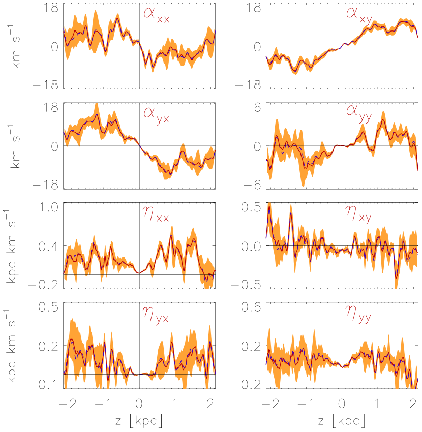
Figure 1: The red solid red lines show the average of the vertical profiles of different dynamo coefficients computed by applying SVD method to nine time different series $S1,S2,...,S9$ during the initial kinematic phase. Orange regions show the $1-\sigma$ variances obtained from these nine different vertical profiles. The inherent error in the SVD estimate of individual coefficients (from Eq.  17) are almost an order of magnitude smaller than the orange regions in the graph. The dashed blue line indicate the vertical profiles of the corresponding coefficients, calculated using the entire time series $S$ in the kinematic phase. We point out that the red solid lines and blue dashed lines almost coincide for all coefficients. Note that $\alpha_{xy}\approx-\alpha_{yx}$ giving rise to a vertical pumping term.

The profiles of all the components of $\alpha_{i\!j}$ and $\eta_{i\!j}$ tensors, recovered using the SVD method, from the various time series are shown in Fig.  1. The solid line in each panel shows the average profile obtained by averaging the individual profiles recovered from the time series $S1$ to $S9$, while the dashed line shows dynamo coefficients obtained from the full time series $S$. We see a close correspondence between these two, showing that the oversampling implicit in the full time series $S$ does not affect the results. In plotting we smooth these profiles over a window of size $100$ pc which corresponds roughly to the turbulent correlation length scales. Also shown in Fig.  1 by the orange shaded regions are the variance obtained in the dynamo coefficients recovered using the time series $S1$ to $S9$. We note that the formal error from the SVD analysis on the $\alpha_{i\!j}$ and $\eta_{i\!j}$ coefficients obtained using Eq. 17 are much smaller than this variance.

We see from Fig.  1 that the overall shapes of the profiles of diagonal $\alpha$ components are linear in the inner disc of approximate $-0.8$ kpc to $0.8$ kpc , and they have the opposite signs above and below the midplane. The magnitude of $\alpha_{yy}$, which is the crucial part of the $\alpha$-effect for the $\alpha-\Omega$ dynamo, is zero at the midplane (as expected) and rises with $z$ to attain a maximum of about $3{\rm\,km\,\,s\,^{-1}}$ by $z=1$ kpc . A curious feature is that $\alpha_{xx}$ is larger and opposite in sign to $\alpha_{yy}$. Another significant result of this analysis is the emergent antisymmetry of $\alpha$ tensor, which is to say that off-diagonal elements are of opposite signs and similar magnitude. As already found previously (Gressel et al., 2008), these two combine, to constitute a turbulent pumping term $\gamma\sim 10$ km s^-1 at the height of $z=1$ kpc that acts to transport mean magnetic fields towards the equator, against the outward advection by the vertical velocity $\overline{U}_{z}$. The profiles of the $\eta$ tensor, as recovered by the SVD method, are expectedly much noisier. The shape of both diagonal components of $\eta$ tensor profiles is approximately inverted bell shaped, with a maximum turbulent diffusivity of $\simeq 10^{26}{\rm\,cm\,^{2}\,s\,^{-1}}$ at a distance of a kpc from the disk midplane. These values compare favorably with theoretical expectations (Shukurov, 2004). The off diagonal component $\eta_{xy}$ oscillates around zero, while curiously $\eta_{yx}$ is also bell shaped, positive and similar to $\eta_{yy}$.

We have also checked the robustness of SVD results in an alternate manner, by inter-comparing the coefficients computed within different sub-intervals of the original time series. In particular, we divide the kinematic phase time series (100 to 1000 Myr ) of mean field, mean current and EMF components, into four sections of equal lengths and compute all dynamo coefficients corresponding to each of these sections, using the SVD method. These four profiles are then used to compute the average profile and the dispersion about the average. In Fig.  2 we show as red-solid curves, the average vertical profiles of the dynamo coefficients, obtained from the four different sub-intervals of kinematic phase. This can be readily compared with blue-dashed curves which shows the same dynamo coefficients, computed for the entire kinematic phase time series (same as the profiles shown in Fig.  1). We see reasonably good agreement between the two curves which shows the robustness of the SVD method and the validity of the assumption that the dynamo coefficients are approximately constant during the kinematic phase. Represented by the shaded orange region is the 1-$\sigma$ interval for these four vertical profiles of dynamo coefficients. They also show that the fluctuation of $\alpha_{i\!j}$ and $\eta_{i\!j}$ with time is larger than the formal error given by the SVD analysis using the full time series.

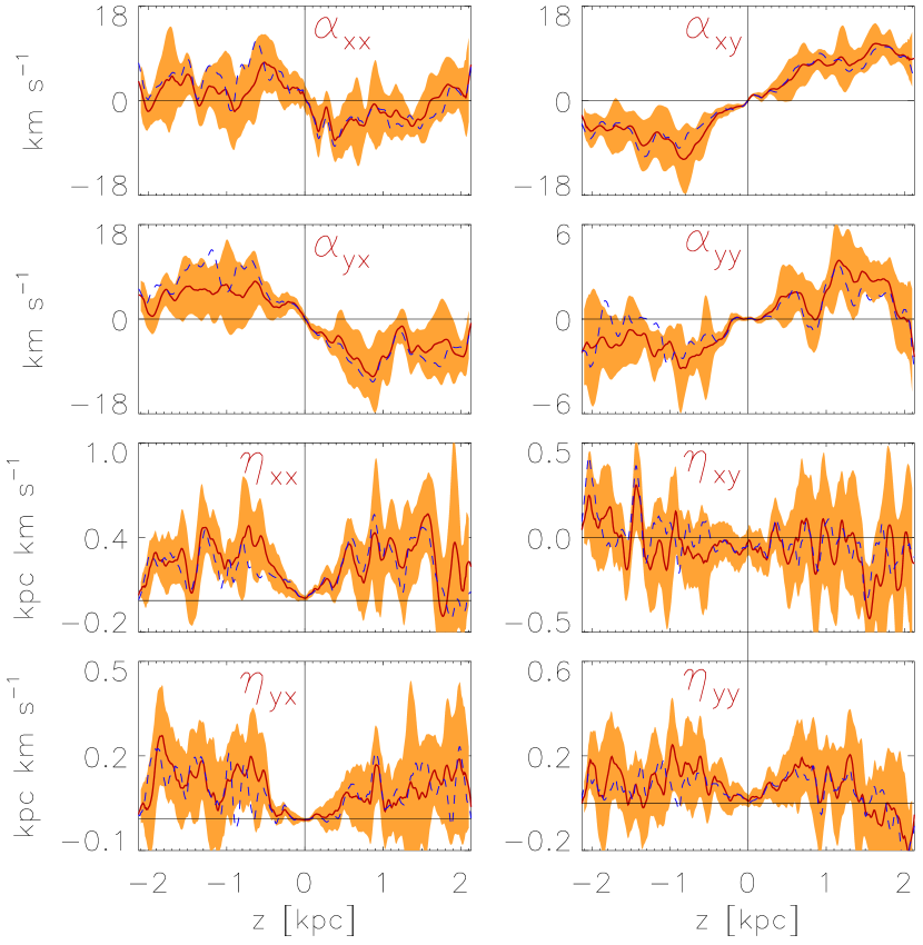
Figure 2: Plotted in the red-solid lines are the average vertical profiles of the dynamo coefficients computed for four different sections of kinematic phase (0.1 to 1  Gyr ) of size 225 Myr . Blue-dashed lines represent the same for respective dynamo coefficients, but for the entire kinematic phase time series, these are identical to the ones shown in Fig.  1. Notice the significant agreement between the red-solid and the blue -dashed curves. Orange regions in each panel represent the corresponding 1-$\sigma$ interval computed using the profiles of dynamo coefficients in the four sections of kinematic phase.

These profiles of dynamo coefficients recovered via SVD are in qualitative agreement with those recovered from TF method for the same model (Bendre et al., 2015; Bendre, 2016). For ready reference we have summarized the TF results derived using the same DNS data in Appendix  B. The magnitude of $\alpha_{yy}$, recovered by the SVD method, is within a $1-\sigma$ confidence interval of its TF counterpart. However the magnitude of $\alpha_{xx}$ from the SVD method is systematically larger by a factor of about 3. Furthermore, a bell shaped profile of both diagonal components of $\eta_{i\!j}$ tensor is obtained in both the SVD and TF methods. The magnitudes of $\eta_{xx}$ and $\eta_{yy}$ however, are substantially smaller in SVD reconstruction, compared to the TF results. One possible explanation for this discrepancy is that the SVD and TF methods, in fact, may be sampling very different length scales in the problem, and that the different values for $\eta$ simply reflect this aspect. We will discuss this issue further in Section 6.

In addition, in Sec.  C the results from the SVD analysis are also compared with that from a simple regression method due to BS02. The mean values of the coefficients obtained in this method are in agreement with that obtained using SVD. The standard deviations tend to be however somewhat larger. Moreover as we will see below, we also use the SVD to compute systematically the full covariance matrix on the coefficients.

4.1 Covariance of the Dynamo Coefficients

In principle, the overdetermined system defined by Eq.  7 has no unique set of solutions in a sense that the same EMF time series could be produced by the different sets of parameters. The SVD algorithm provides a solution that is the best approximation in a least-squared sense. There however could be a degeneracy in the determination which could be probed quantitatively by comparing the off-diagonal elements of covariance matrix to the diagonal ones. Since the time series of both $x$ and $y$ components of EMF (columns of $\mathcal{Y}$) depend on the first and second column of $\mathcal{X}$ through the same design matrix $\mathcal{A}$ covariance between the elements of $\hat{\mathbf{x}}_{1}$ and $\hat{\mathbf{x}}_{2}$ are identical (see Eq.  15) and following relations hold:

$$\mathrm{Cov}\Big{(}\alpha_{xx},\alpha_{xy}\Big{)}=\mathrm{Cov}\Big{(}\alpha_{yx},\alpha_{yy}\Big{)}\,,$$

$$\mathrm{Cov}\Big{(}\alpha_{xx},\eta_{xx}\Big{)}=\mathrm{Cov}\Big{(}\alpha_{yx},\eta_{yx}\Big{)}\,,$$

$$\mathrm{Cov}\Big{(}\alpha_{xx},\eta_{xy}\Big{)}=\mathrm{Cov}\Big{(}\alpha_{yx},\eta_{yy}\Big{)}\,,$$

$$\mathrm{Cov}\Big{(}\alpha_{xy},\eta_{xx}\Big{)}=\mathrm{Cov}\Big{(}\alpha_{yy},\eta_{yx}\Big{)}\,,$$

$$\mathrm{Cov}\Big{(}\alpha_{xy},\eta_{xy}\Big{)}=\mathrm{Cov}\Big{(}\alpha_{yy},\eta_{yy}\Big{)}\,,$$

$$\mathrm{Cov}\Big{(}\eta_{xx},\eta_{xy}\Big{)}=\mathrm{Cov}\Big{(}\eta_{yx},\eta_{yy}\Big{)}\,.$$

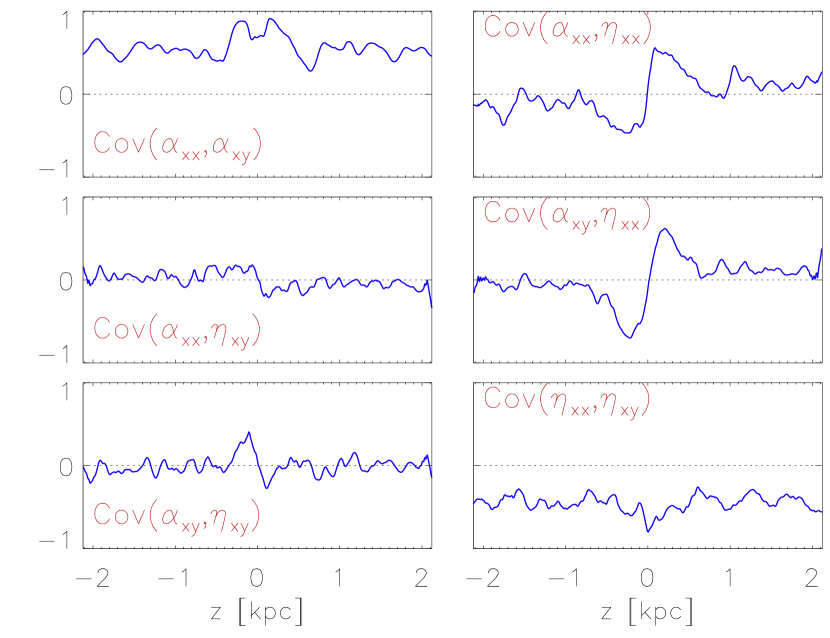
Figure 3: Vertical profiles of all off-diagonal elements of covariance tensor normalized with their respective diagonal components.

In Fig.  3, we plot the vertical profiles of the off-diagonal elements of the covariance matrix (calculated using Eq.  15) normalized with the corresponding diagonal elements. If two parameters are uncorrelated the corresponding normalized covariance will be zero, full correlation corresponds to $+1$ and complete anti-correlation to $-1$. From this figure, we see that the diagonal and off-diagonal elements of the $\alpha_{i\!j}$ tensor, like $\alpha_{xx}$ and $\alpha_{xy}$ (or $\alpha_{yy}$ and $\alpha_{yx}$) are correlated for all $z$, while the corresponding diagonal and off-diagonal elements of the $\eta_{i\!j}$ tensor are anti-correlated (see the top-left and bottom-right panels of Fig.  3). Moreover, the correlations between the first and third element and the second and the fourth element of $\hat{\mathbf{x}}_{i}$ (equivalently $\mathrm{Cov}\left(\alpha_{xx},\eta_{xx}\right)$ and $\mathrm{Cov}\left(\alpha_{yy},\eta_{yy}\right)$ are non negligible within the central half a kpc of the disk, where the mean field is strong.

These correlations can arise if there are definite correlations between the mean field components with themselves and with the current components. For example if we have a definite eigenmode of the mean-field dynamo with say $\overline{B}_{y}\approx-c_{1}\overline{B}_{x}$, with a constant $c_{1}$. Then $\overline{\mathcal{E}}_{x}=\alpha_{xx}\overline{B}_{x}+\alpha_{xy}\overline{B}_{y}+...\approx(\alpha_{xx}-c_{1}\alpha_{xy})\overline{B}_{x}+....$, and there can be a mixing (or correlation) between $\alpha_{xx}$ and $\alpha_{xy}$, as indeed observed. Similarly, if the field is partially helical, then there would be a correlation between $\overline{B}_{x}$ and $\overline{J}_{x}$ (also $\overline{B}_{y}$ with $\overline{J}_{y}$). This could indeed induce a partial correlation between $\alpha_{xx}$ and $\eta_{xx}$ (and $\alpha_{yy}$ with $\eta_{yy}$), as also indeed observed in the top right panel of Fig.  3.

We see therefore that all the turbulent dynamo coefficients determined by the SVD, by directly fitting the $\overline{\mathbf{\mathcal{E}}}$ data from the numerical simulation, need not be completely independent. This will be the case if the mean fields and currents are partially correlated. The coefficients determined by the SVD do however give the best fit to the data in a least-squared sense. This also explains why the TF results and the SVD method, even if they differ somewhat in the amplitudes of different coefficients, could lead to very similar $\overline{\mathbf{\mathcal{E}}}$ and hence predict similar evolution for the mean field evolution.

4.2 Quenching of the Dynamo Coefficients

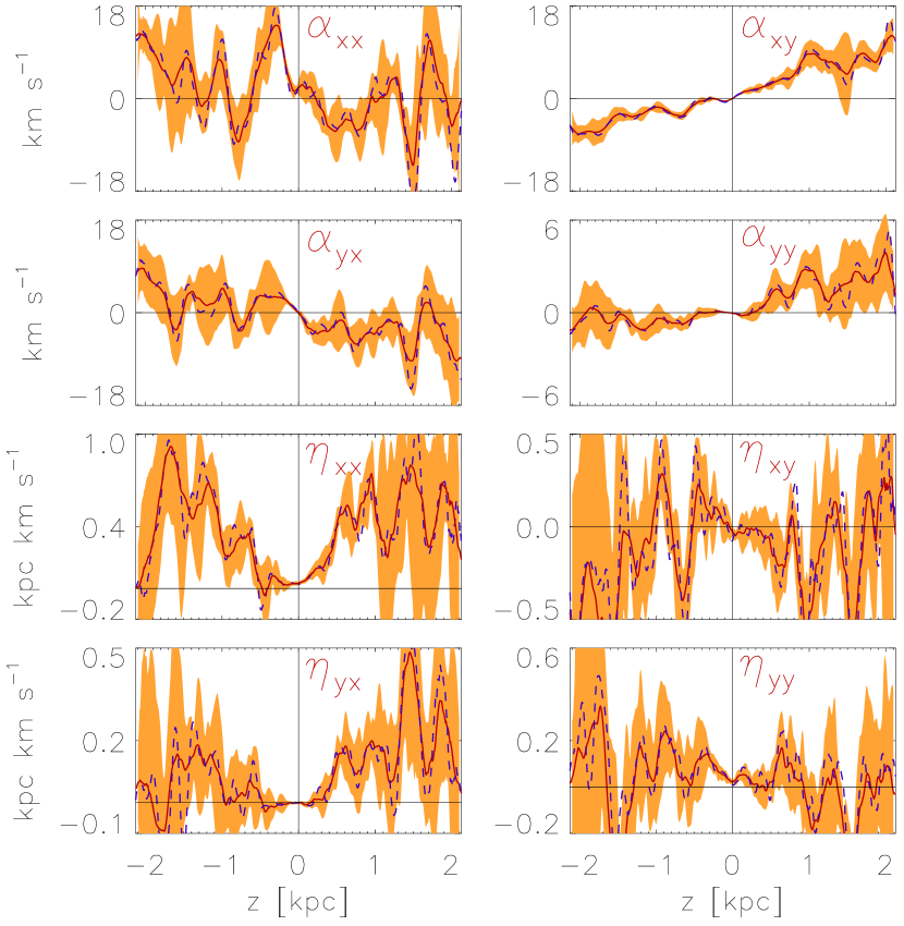
Figure 4: Same as Fig.  1 but for the dynamical phase.

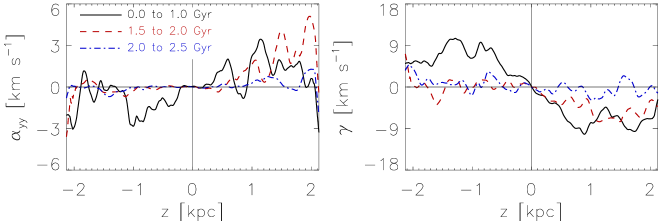
Figure 5: Left Panel: Vertical profile of the $\alpha_{yy}$ coefficient in the kinematic (black-solid line), the dynamical phases ($1.5$ - $2.0$) Gyr (red-dashed line) and ($2.0$ - $2.5$) Gyr (blue-dash-dotted line). Right Panel: shows the same but for turbulent pumping (i.e., $\gamma$) term with the same colour coding.

It is of interest to examine the behaviour of the dynamo coefficients as the mean magnetic field grows and Lorentz forces become important. Our previous analysis based on the TF method (Gressel et al., 2013; Bendre, 2016) indicated that both $\alpha$ and $\eta$ coefficients quench drastically in the presence of dynamically significant mean fields as an algebraic function of relative field strengths. We perform a similar analysis using SVD method here. To quantify the strengths of the mean fields relative to turbulent kinetic energy we use the dimensionless ratio of the magnetic to kinetic energy defined by,

$$\beta^{2}=\frac{\overline{\mathbf{B}}\cdot\overline{\mathbf{B}}}{\mu_{0}\,\rho\,u^{2}}\,.$$ (19)

To investigate the effect of strong mean field on the dynamo coefficients, we examine their behaviour at two regions of $\beta$. We choose the time series of $\overline{\mathbf{B}}$, $\overline{\mathbf{J}}$ and $\overline{\mbox{\boldmath${\cal E}$}{}}$ from DNS, corresponding to $0.1$ to $1$ Gyr representing its initial kinematic phase ($\beta\leq 0.01$). Conversely, for the dynamical phase ($\beta\geq 1$) we use the time series between $1.5$  Gyr and $2.54$ Gyr . Equipped with this data, we compute vertical profiles of all dynamo coefficients using the SVD method as discussed in the previous section.

It should be noted that, the SVD algorithm we have employed requires the dynamo coefficients to stay constant for a chosen range of time. Consequently while choosing the time slots at various values of $\beta$ we are tacitly assuming the constancy of dynamo coefficients for that range. This assumption may be justifiable in the kinematic phase where the exponential growth of magnetic is consistent with the solution of $\alpha-\Omega$ dynamo with constant dynamo coefficients. Moreover, in the dynamical phase above $\sim 1.5$ Gyr , the average growth of mean fields appears to be approximately exponential, however with a drastically reduced growth rate. This also hints the existence of dynamo action with a set of approximately constant (but quenched) dynamo coefficients. For the intermediate phase of approximately 1.0 and 1.5 Gyr however, where the transition between kinematic and quenched dynamo coefficients is supposed to occur, the constraint of the constancy may not hold. We therefore focus here on the dynamo coefficients in the kinematic and dynamical phase using this method, and not in the intermediate phase of transition.

The dynamo coefficients in the dynamical phase are shown in Fig.  4. The plots show a drastic suppression of the mean $\alpha_{yy}$ and the off-diagonal terms, $\alpha_{xy}$ and $\alpha_{yx}$, for $z<0$, which in turn implies a drastic suppression of the pumping term $\gamma=\left(\alpha_{yx}-\alpha_{xy}\right)/2$. It appears that the mean value of these coefficients are less affected for $z>0$. However, the lower envelope of $\alpha_{yy}$ is closer to zero in the dynamic phase compared to the kinematic phase, even for $z>0$. We find that the other coefficients do not undergo any systematic quenching, although the variance in these coefficients are much larger in the dynamic compared to the kinematic phase and it is harder therefore to quantitatively determine the quenching.

To elucidate the behaviour of the dynamo coefficients in the dynamical phase further, we have split this period in to two sub-periods, $1.5$ to $2$  Gyr , and $2$ to $2.5$ Gyr. In Fig.  5 we compare the vertical profiles of $\alpha_{yy}$ and $\gamma$ coefficients for these two dynamical regimes with the kinematic regime. The figures show clearly, that for the final period of $2$ to $2.5$ Gyr, the suppression of $\alpha_{yy}$ and the pumping term $\gamma$ is now drastic for all values of $z$, This also shows that the turbulent coefficients are evolving in the dynamic phase and Fig.  4 shows the average behaviour, assuming they are constant.

Note that in the kinematic stage the $\gamma$ term pumped back the mean field into the disk part, which an outflowing wind was carrying out in the halo. The decrease of $\alpha_{yy}$ and $\gamma$ could therefore be the cause of dynamical saturation of magnetic field seen in the DNS. We should also point out that the mean vertical velocity $\overline{U}_{z}$ is suppressed as the $\beta$ or the mean magnetic field increases, as already shown in Bendre, Gressel & Elstner (2015).

4.3 Comparison of recovered $\overline{\mbox{\boldmath${\cal E}$}{}}$ with the DNS

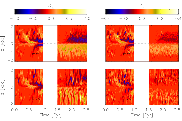
Figure 6: Left Panels: Bottom panel shows the time evolution of the vertical profile of $\overline{\mathcal{E}}_{x}$ obtained from the DNS and the top panel depicts the same for the $x$ component of reconstructed EMF using the SVD estimates of $\alpha$ and $\eta$ tensors and the profiles of mean field components from DNS. Right Panels: Show the same quantities as the left one but for the $y$ component of EMF. Note that the SOCA the model for EMF components roughly reproduces the actual DNS data. The white patch ranging from 1 to $1.5$ Gyr corresponds to the transition phase between the kinematic and dynamical phase of field evolution, since the dynamo coefficients in this range cannot be reliably extracted by present SVD method, we have omitted this patch in this comparison. Color code here is normalized with respect to the exponential scaling factor of $\exp{\left(t/200{\rm Myr}\right)}$, in the kinematic phase to compensate for the exponential amplification of EMF components as mentioned in Sec.  3.2.

It is important to ask how well $\overline{\mbox{\boldmath${\cal E}$}{}}$, obtained from the turbulent transport coefficients recovered with the SVD method according to Eq.  4 or Eq.  7 agrees with $\overline{\mbox{\boldmath${\cal E}$}{}}$ in the DNS and what is the level of residual noise in this fit. We compare in Fig.  6 the evolution of $\overline{\mathcal{E}}_{x}\left(z\right)$ and $\overline{\mathcal{E}}_{y}\left(z\right)$ obtained from the DNS (Bottom panels) with that reconstructed using the SVD estimates of the $\alpha_{i\!j}$ and $\eta_{i\!j}$ tensors (top panels). We see that that there is reasonable agreement between the two, especially in the kinematic stage.

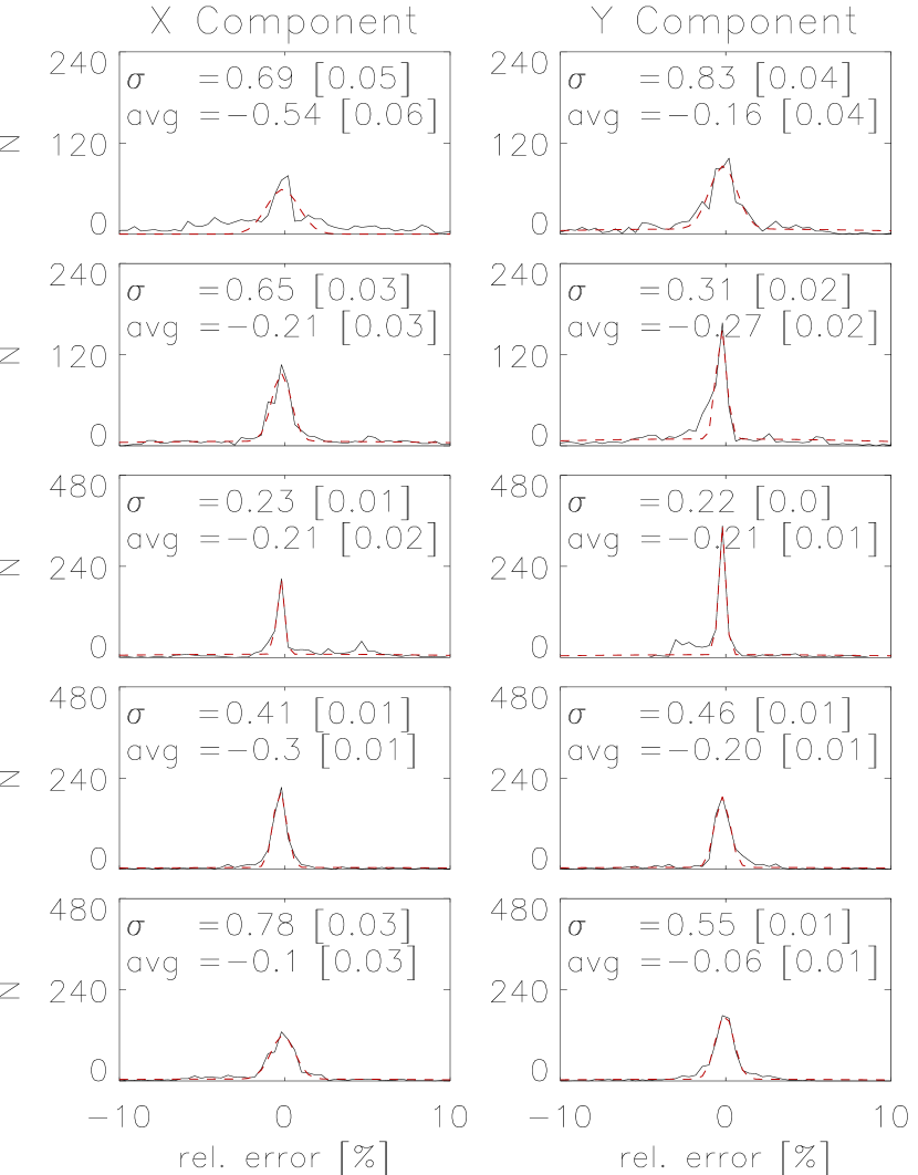
Figure 7: Black-solid lines show the residual noise ‘probability’ distributions obtained by subtracting the kinematic phase time series of $\overline{\mathbf{\mathcal{E}}}$ obtained in the SVD reconstruction from that obtained in the DNS. The noise is expressed in the units of percentage of the DNS $\overline{\mathbf{\mathcal{E}}}$ value. The red lines show the Gaussian best fit of the respective distributions. Mean (avg) and standard deviation ($\sigma$) of each fit is given in each box and the square brackets show the errors in their determination.

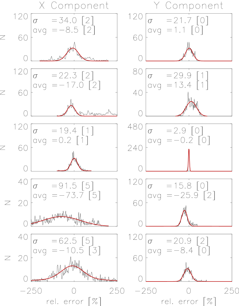
Figure 8: Same as Fig.  7 but for the dynamical phase time series (restricted to the time period of $t\geq 1.5$ Gyr ) of EMF components.

In order to make this comparison more quantitative and estimate the level of the residual noise in the SVD fit, we have also compared the time-series of both components of EMF obtained from the DNS ($\overline{\mathcal{E}}_{i}=\overline{\left(\mathbf{u}\times\mathbf{b}\right)_{i}}$) and the ones reconstructed using the dynamo coefficients ($\overline{\mathcal{E}}_{i}=\alpha_{i\!j}\overline{B}_{j}-\eta_{i\!j}\overline{J}_{j}$) at specific locations. This is shown in Fig.  7 and Fig.  8, where we plot the histograms of the relative differences (in percentage) between $x$ and $y$ components of EMF obtained from the DNS and corresponding estimates using SVD, for the kinematic ($0.1$ to $1$ Gyr ) and the dynamical phase (above $1.5$  Gyr ) respectively. The left and right panels of each figure, correspond respectively to the distribution of this residual noise in the $x$ and $y$ components of EMF. We do this analysis at various heights and the panels from bottom to top show the results at $z=-1$ kpc , $-0.5$  kpc , $0$ kpc , $0.5$ and $1.0$  kpc . We see that the relative difference between the two is mostly normally distributed at all heights. We then fit these histograms with the Gaussian functions (shown with red curves), and determine both the mean and the dispersion $\sigma$ of the distributions.

We see from Fig.  7 that the mean of the residual noise is very close to zero during the kinematic phase, while their $\sigma$ values turn out to be less than a few percent at all locations. Therefore the reconstructed EMF using the SVD method does give a good fit to that obtained directly in the simulations during the kinematic evolution. On the other hand, both the mean residual noise and its dispersion are larger during the dynamical phase as can be seen from Fig.  8. The mean noise ranges from a few percent to 30% for the $y$ component of the EMF with the dispersion $\sigma$ less than 30%. For the $x$ component, the mean residual noise has a similar range except around $z\sim-0.5$ kpc where it becomes as much as 70%. The dispersion in the noise is also larger at this location. At all heights, however the zero value is within the 1-$\sigma$ range of the noise distribution. These features indicate that while the SVD method provides an excellent fit in the kinematic phase, it is not providing as good a fit in the dynamical phase. At the same time, we shall see in Section 5 that the a 1-D mean field dynamo model using the turbulent dynamo coefficients obtained from the SVD method reproduces reasonably well the evolution of the mean magnetic field, not only in the kinematic phase but also in the dynamical phase.

5 Comparison of one-D dynamo model with the DNS

The validity of the computed profiles of dynamo coefficients in the kinematic and dynamical phase can also be verified, self-consistently, by demonstrating that a 1-D dynamo model using these coefficients gives results very similar to the DNS. The 1-D dynamo equations are,

$$\frac{\partial\overline{{B}}_{x}}{\partial t} =\frac{\partial}{\partial z}\Bigg{(}-\left(\overline{U}_{z}+\alpha_{yx}\right)\overline{{B}}_{x}-\alpha_{yy}\,\overline{{B}}_{y}-\eta_{yy}\,\overline{{J}}_{y}-\eta_{yx}\,\overline{{J}}_{x}\Bigg{)}$$

$$\frac{\partial\overline{{B}}_{y}}{\partial t} =\frac{\partial}{\partial z}\Bigg{(}-\left(\overline{U}_{z}-\alpha_{xy}\right)\overline{{B}}_{y}+\alpha_{xx}\,\overline{{B}}_{x}+\eta_{xx}\,\overline{{J}}_{x}-\eta_{xy}\,\overline{{J}}_{y}\Bigg{)}$$

$$+q\,\Omega\,\overline{{B}}_{x}.$$ (20)

Note that from $\nabla\cdot{\mathbf{B}}=0$, $\overline{B}_{z}=\rm const.$ for the $x-y$ averaged mean. We solve Eq.  20 with a resolution of 512 grid points similar to the DNS. Adopting a continuous gradient boundary condition for $\overline{B}_{x}$ and $\overline{B}_{y}$, we evolve Eq.  20 on a staggered grid using the finite difference method. Initial profiles of $\overline{B}_{x}$ and $\overline{B}_{y}$ components are taken directly from the respective DNS data averaged over first $150$ Myr .

The vertical profiles of dynamo coefficients used for the first gigayear are as determined from the SVD analysis and given in Fig.  1. For the latter period of 1 to $1.5$  Gyr , we use the linearly interpolated profiles of $\alpha_{yy}$ and pumping term between black-solid and blue-dashed curves shown in Fig.  5 to roughly mimic the transition between kinematic and dynamical phases and keep other coefficients the same. For the period after $1.5$ Gyr , to simulate the dynamical quenching of the coefficients, we further replace these with the once shown in Fig.  5 with blue-dashed curves and keep the rest of the coefficients constant. We run this model up to $2.54$ Gyr .

Figure 9: Left Panel: Black-solid lines show the vertical profile of $\overline{{B}}_{y}$ seen in the DNS, while its dashed counterparts show the same for 1D dynamo model. The approximately symmetric profiles with respect to the midplane corresponds to the $\overline{{B}}_{y}$ at end of dynamical phase, 2.5  Gyr , and the antisymmetric ones correspond to 0.8 Gyr . Right Panel: The black-solid line represents the time evolution of the mean-magnetic energy expressed in logarithmic units for the DNS, while the dashed line represents the same for 1-D model.

The results of these simulations are shown in Fig.  9, and Fig.  10. After an initial period of $\sim 80$ Myr when the initial transients decay, the overall evolution of magnetic field in 1-D model is reasonably consistent with the outcome of the DNS. To corroborate this, in Fig.  9 (right panel) we first compare the time evolution of mean magnetic energies in DNS (shown with solid line) and 1-D simulations (shown with dashed line). We see that mean magnetic energy curves from the direct and 1-D simulations, overlap closely both in kinematic and dynamical phase. This clearly shows the overall similarity in the magnetic energy growth, with the e-folding time of $\sim 100$ Myr in the kinematic and $\sim 520$ Myr in the dynamical phase as in the DNS. Furthermore, in Fig.  10 we compare the space-time butterfly diagrams of azimuthal field component ($z-t$ evolution). This also shows the qualitative similarity with which the field profile is reproduced along with the reversals and the emergence of final symmetric mode. To supplement this, we additionally compare in Fig.  9 (left panel) the vertical profiles of $\overline{B}_{y}$ from DNS (solid lines) and 1-D simulations (dashed lines) at an intermediate time of $0.8$ Gyr (when there obtains an antisymmetric mode with respect to the mid-plane) and near the end of the simulation at $2.5$ Gyr , (when a symmetric mode is prevalent). This comparison also shows that the approximate shape of the $\overline{B}_{y}$ profile is well replicated in 1-D dynamo simulations. Overall, the similarity in the evolution of the mean magnetic field in the DNS and 1-D models which uses the dynamo coefficients determined using SVD method supports the robustness of the chosen approach.

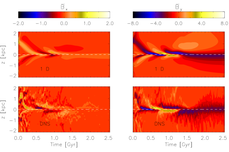
Figure 10: Left Panel: Shows the time evolution of the vertical profile of $\overline{B}_{x}$ seen in the DNS (bottom panel), and in the 1D dynamo model (top panel) Right Panel: Shows the same but for the $y$ component of mean field. We have normalized the colour code with mean magnetic energy to compensate for the exponential amplification of mean field and make its initial features visible.

6 Discussion and Conclusions

The determination of turbulent transport coefficients in direct simulations which give rise to large-scale dynamo action is important to understand how the dynamo operates to grow and maintain the large-scale magnetic fields. Several methods have been suggested in the past, including what is known as the test-field (TF) method and the singular value decomposition (SVD) method. The SVD is useful particularly for post processing analysis of simulation data.

We have presented in this paper a SVD analysis of the simulation of SNe driven ISM turbulence of Bendre, Gressel & Elstner (2015), which had led to large-scale field generation. TF results for this simulation have been presented there, which makes it also possible to compare the results obtained from these two very different methods. The profiles of dynamo coefficient tensors $\alpha_{i\!j}(z)$ and $\eta_{i\!j}(z)$ in the SVD method are obtained from the turbulence data by minimising the least squares of a residual vector $R_{i}=\overline{\mathcal{E}}_{i}-\alpha_{i\!j}\,\overline{B}_{j}+\eta_{i\!j}\,\overline{J}_{j}$. As a consistency check we verify the efficacy of SVD algorithm in Appendix  A and by using the exact data produced in 1-D simulations, adding random white noise up to a level of 50% of the actual data, and showing that the SVD effectively reconstructs the dynamo coefficient tensors. The profiles of $\alpha_{i\!j}(z)$ and $\eta_{i\!j}(z)$ tensors, calculated using the SVD method, are shown in Fig.  1 for the kinematic phase and Fig.  4 for the dynamical phase when the dynamo growth has decreased. We also show that the turbulent EMF components predicted using the reconstructed $\alpha_{i\!j}$ and $\eta_{i\!j}$ tensors match quite well with actual DNS data for the kinematic phase, with very little residual noise. The match is not as good for the dynamical phase. However, we show that the evolution of the mean magnetic fields, predicted by solving the 1-D mean-field dynamo equations using the reconstructed dynamo coefficients match remarkably well, with that determined from the DNS, as can be seen from Fig.  9 and Fig.  10. Thus it seems that the SVD does indeed give a reasonable reconstruction of the dynamo coefficients.

The predicted magnitude of $\alpha_{yy}$, crucial for regenerating $\overline{B}_{x}$ from $\overline{B}_{y}$ in the $\alpha-\Omega$ dynamo, is zero at the midplane (as expected) and rises with $z$ to attain a maximum of about $3{\rm\,km\,\,s\,^{-1}}$ by $z=1$  kpc . We also predict a turbulent pumping term $\gamma\sim 10$ km s^-1 at the height of a  kpc , that acts to transport mean fields towards the equator, against the outward advection by the vertical velocity $\overline{U}_{z}$. The diagonal components of turbulent diffusion tensor, as recovered by the SVD method, are much more noisy, approximately inverted bell shaped, with a maximum turbulent diffusivity of $\simeq 10^{26}{\rm\,cm\,^{2}\,s\,^{-1}}$ at a distance of a  kpc from the disk midplane. These numbers compare favorably with that expected on basis of simple estimates for galactic dynamos (Shukurov, 2004). We find that as the mean field becomes stronger, both $\alpha_{yy}$ and $\gamma$ get suppressed, but other coefficients remain largely unaltered.

The vertical profiles of all dynamo coefficients constructed in SVD analysis (Fig.  1) are qualitatively similar to their TF counterparts (shown in Fig.  13) during the kinematic phase. In this phase, they are also similar to that obtained from a simple regression method of BS02, as shown in Fig.  14. The amplitude of $\alpha_{xx}$ however is larger by a factor of 3 as determined in the SVD analysis compared to the TF method, while $\eta_{xx}$ and $\eta_{yy}$ are substantially smaller. We stress that the SVD method is likely most sensitive to vertical gradients in the mean fields on relatively smaller scales. This is because it is restricted to the length scales that are actually sampled from the fields present in the DNS, which are confined to a few hundred parsec around the midplane. In contrast, the TF method (in its form used here) is essentially a spectral method, where one is free to choose the length scale probed. It has to be noted that the particular choice was to have test fields that vary on the largest vertical scales accessible in the tall simulation domain. Gressel & Pessah (2015) have demonstrated the scale-dependence of the TF coefficients for the case of magnetorotational turbulence, where coefficients were found to decay from their peak value at the largest available scales by a factor of a few, when approaching the smallest scales accessible to the simulation. This scale-dependence may in fact fully explain the tension between the SVD and TF results, which can be tested by running the latter method at higher vertical wavenumber.

In the dynamically quenched phase, the TF method predicts not only suppression of $\alpha_{yy}$ and $\gamma$ but also the turbulent diffusion tensor, with the latter feature not having been clearly obtained in the SVD analysis. Nevertheless, the 1-D model using the TF results had also matched the evolution of the mean magnetic fields obtained in the DNS (Bendre, Gressel & Elstner, 2015). This seems to indicate a degeneracy in the determination of the magnitudes of turbulent transport coefficients using different methods. A potential explanation for this feature is the existence of partial correlations between some of the parameters, as explicitly shown in Fig.  3.

Our work here has demonstrated that the SVD method is a self-consistent and useful way of determining turbulent transport coefficients. In contrast to the TF method, it is computationally less expensive since it is used merely as a post-processing tool. However, as a potential downside of the SVD method, some of the determined parameters can also get correlated if the different components of the mean fields and currents have definite correlations. The reconstruction of coefficients which couple to the current is also more noisy in the SVD method. These latter issues are tacitly avoided in TF method as they study the inductive response to known functional forms of additional mean test fields. The TF method itself is believed to have difficulties in dealing with a strong small-scale dynamo, where small scale fields are generated independent of the mean magnetic field. Here such fields will merely appear as an extra noise term to be recovered self-consistently in the SVD reconstruction. It will be important to study a case where both large and small-scale dynamos are active (e.g., the case in Bhat et al. (2019)), with the SVD method. Also of interest will be to recover the dynamo coefficients when the mean field is defined differently, like in the filtering approach (eg. Gent et al. (2013)). In addition, it would be useful to be able to implement Bayesian priors for the dynamo coefficients, perhaps using the information field theory approach (e.g., Enßlin, 2019), while doing the least-square minimisation of the data; a study which is left for the future.

Appendix A Testing the SVD method using mock data

To verify the robustness and predictive ability of the SVD method for the problem of mean-field dynamo, we use mock data of the mean magnetic fields produced in 1D dynamo simulations using the profiles of dynamo coefficients (described in Sec.  5). We extract the time series data of $\overline{B}_{x}\left(z,t\right)$ and $\overline{B}_{y}\left(z,t\right)$ and add the various levels of normally distributed random noise over these time series. We denote these noisy components $\overline{B}^{n}_{x}$ and $\overline{B}^{n}_{y}$. To then compute the time series of noisy mean current components $\overline{J}_{x}^{n}$ and $\overline{J}_{y}^{n}$ we filter the data $\overline{B}^{n}_{x}\left(z,t\right)$ and $\overline{B}^{n}_{y}\left(z,t\right)$ using moving windows of width $\sim 80$ pc in $z$ direction and $\sim 60$  Myr in $t$ direction, and calculate the components of$\nabla\times\overline{\mathbf{B}}^{n}$. Similarly we also construct the time series of $\overline{\mathcal{E}}_{x}$ and $\overline{\mathcal{E}}_{y}$ from the exact profiles of $\overline{B}_{x}$, $\overline{B}_{y}$, $\overline{J}_{x}$, $\overline{J}_{y}$ and the dynamo coefficients obtained by SVD. By adding the same levels of noise over $\overline{\mathcal{E}}$, and then filtering with same window size the time series $\overline{\mathcal{E}}^{n}$ components are constructed. Using these noisy time series $\overline{\mathbf{B}}^{n}$, $\overline{\mathbf{J}}^{n}$ and $\overline{\mathcal{E}}^{n}$, we subsequently follow the steps described in Sec.  3.2 to pseudo-invert the design matrix $\mathbf{A}$ at each $z$ and reconstruct the profiles of all dynamo coefficients, along with their variances. In Fig.  11 we show the reconstructed profiles of the dynamo coefficients with a level of added noise equaling to approximately $50\%$ of the actual data (with black lines). Here we point out that noise dispersion in the actual DNS data in its kinematic phase is almost an order of magnitude smaller than the value we use here. It is however almost similar to the expected noise in dynamical phase (see Fig.  7 and Fig.  8). The red curves in Fig.  11 show actual profiles of dynamo coefficients for non-noisy data set.

It can be seen from the figure that the predictions of $\alpha$ tensor components agree remarkably well with the input profiles. They are considerably better than the predictions of $\eta_{ij}$, especially for the off diagonal component $\eta_{xy}$. We also find that if we neglect the off diagonal components of $\eta$ tensor altogether, this further improves the SVD predictions for both $\alpha$ and diagonal elements of $\eta$. Qualitative consistency of the reconstructed profiles with the actual profiles justifies the robustness of SVD algorithm.

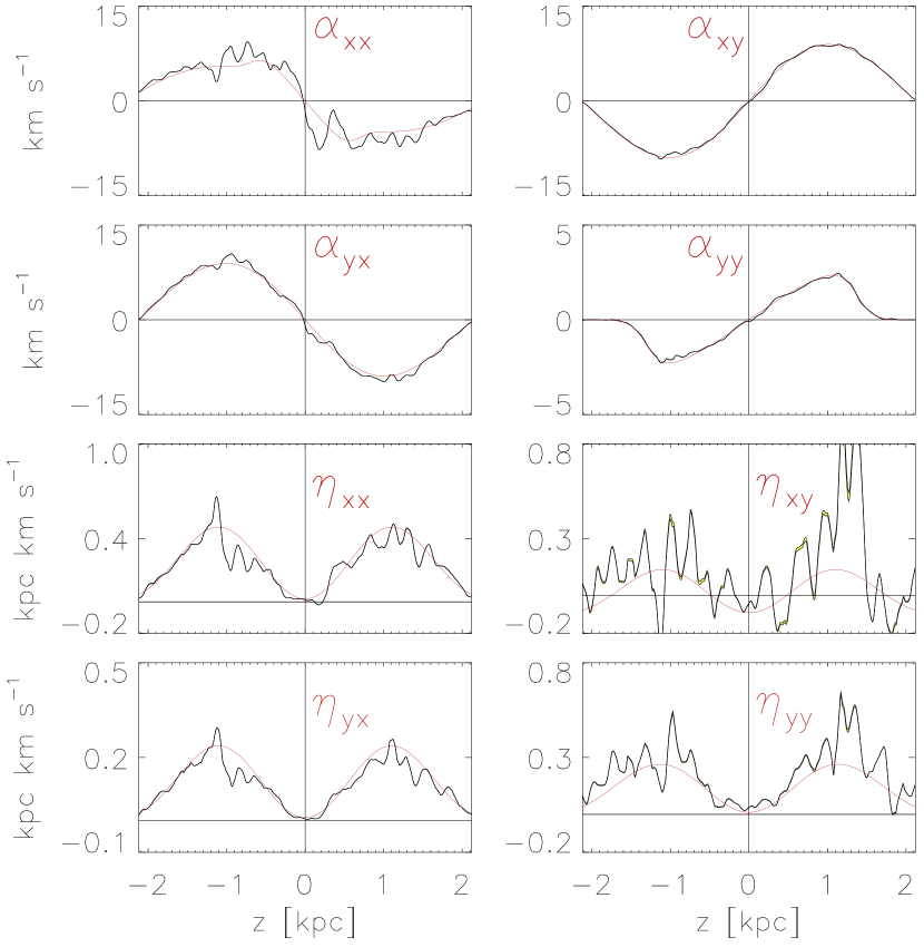
Figure 11: Black-lines show the vertical profiles of all dynamo coefficients reconstructed from 1D dynamo data with added noise level of 50% to the actual data. Red-lines show the dynamo coefficients actually used in the 1D Dynamo simulations.

One of the main sources of errors in determining the dynamo coefficients using SVD algorithm is the enhancement of noise when determining $\overline{\mathbf{J}}^{n}$ due to taking the derivative of the noisy mean field data. Large relative errors are introduced in the derivatives of $\overline{\mathbf{B}}$ where it is expected to have a negligible gradient. To circumvent this issue, we also define the components of $\overline{\mathbf{J}}^{n}$ as the discrete inverse Fourier transforms of $\overline{J}_{x}^{n}\left(k\right)$ and $\overline{J}_{y}^{n}\left(k\right)$ defined by

$$\overline{J}_{x}^{n}\left(k\right) =\frac{2\pi ik}{N}\sum_{z}\overline{B}_{y}^{n}\left(z\right)\,\mathrm{exp}\left(\frac{-2\pi ikz}{N}\right)$$

$$\overline{J}_{y}^{n}\left(k\right) =-\frac{2\pi ik}{N}\sum_{z}\overline{B}_{x}^{n}\left(z\right)\,\mathrm{exp}\left(\frac{-2\pi ikz}{N}\right).$$ (21)

Resulting time series of $\overline{\mathbf{J}}^{n}$, $\overline{\mathbf{B}}^{n}$ and $\overline{\mbox{\boldmath${\cal E}$}{}}^{n}$ is then used to determine the dynamo coefficients corresponding to noisy data, using the SVD method described above. This exercise also yields the results consistent with the actual values of dynamo coefficients even with added noise level of $\sim 50\%$ of actual data, as shown in Fig.  12. These tests with mock data show that the dynamo coefficients can be reasonably well recovered using the SVD method. It also shows that the recovering the $\eta_{i\!j}$ tensor accurately is more difficult compared to recovery of the $\alpha_{i\!j}$ tensor.

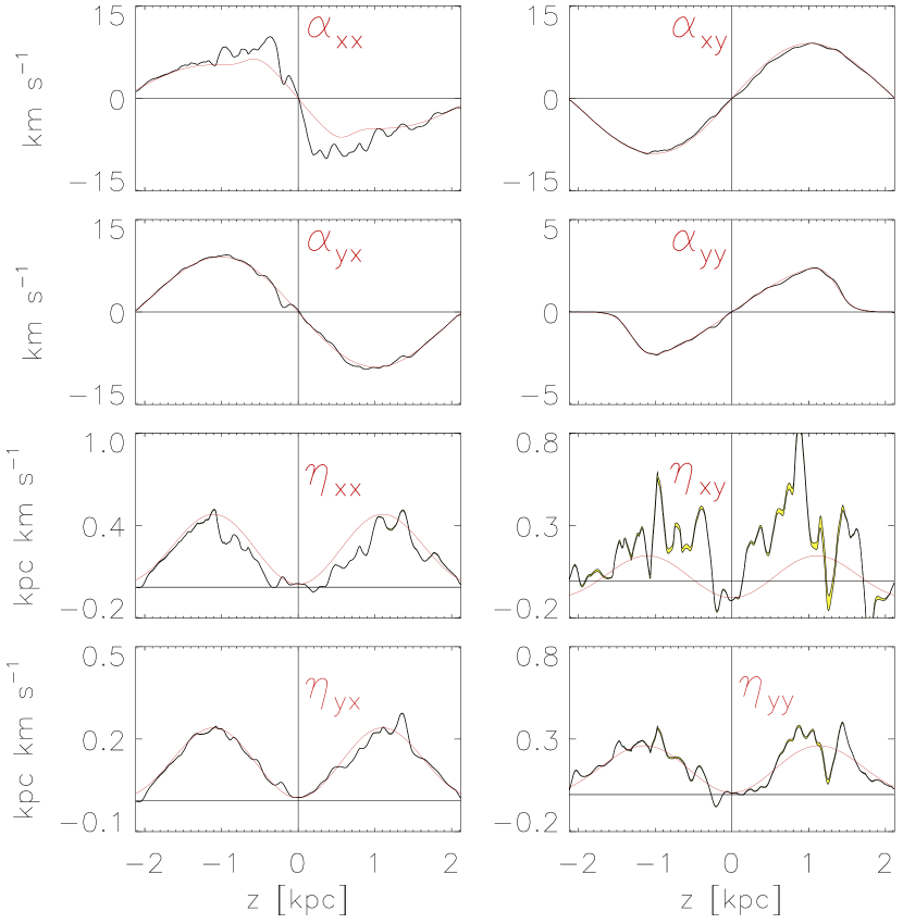
Figure 12: Same as Fig.  11, but with currents components calculated using Eq.  21

Appendix B Test-Field Results

In order to solve the system represented by Eq.  4 for $\alpha$ and $\eta$ tensors, in our previous work we use the TF method discussed by Brandenburg (2018). A general idea of the TF is as follows: Since the Eq.  4 is an under-determined system with two equations and eight unknowns, one needs sufficient number of independent equations to invert it. In the TF method, this is achieved by solving the induction equation for additional passive test fields with a well defined functional form along with the DNS, as described briefly in Section 1. Fluctuations in these fields are then computed as functions of space and time and used to compute the TF EMF components. With this additional data Eq.  4 is inverted to compute the unknown $\alpha$ and $\eta$ tensors. Analysis of the DNS model used in this paper (model Q) based on the TF results is discussed in details in Bendre, Gressel & Elstner (2015). For the sake of comparison with the SVD analysis, in Fig.  13 we plot the vertical profiles all dynamo coefficients obtained from the TF analysis of the same model in solid red lines, along with 1-$\sigma$ error estimates represented by the orange shaded regions.

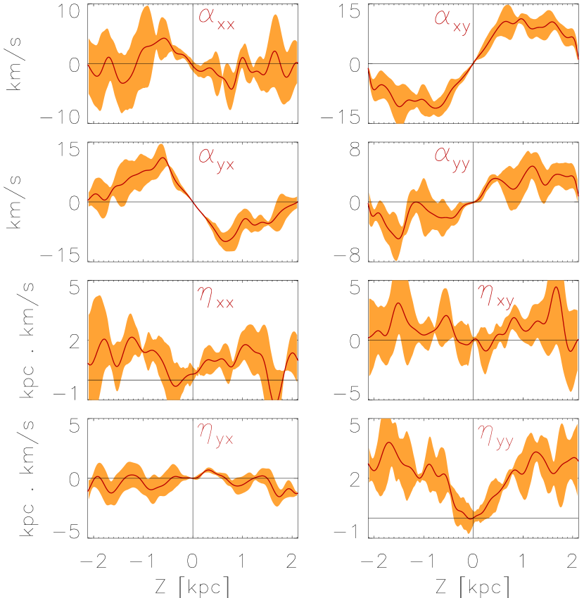
Figure 13: Plotted here are the vertical profiles of all dynamo coefficients obtained from TF in red-solid lines and corresponding 1-$\sigma$ error estimates shown by the overlayed orange shaded areas. These results correspond to the exponential amplification phase of mean fields $t\in(0.1:0.8)$  Gyr , similar to the SVD results presented in Fig.  1. Vertical profiles are also Fourier filtered such that all the fluctuations below the estimated turbulent correlation length scales of $\sim 100$  pc are eliminated.

Here we have presented the TF results only in the kinematic regime of field evolution. Changes in these profiles in the presence of dynamically significant mean fields are discussed in Bendre, Gressel & Elstner (2015) and in Section 5.3.2 of Bendre (2016). Qualitative trends of these profiles of dynamo coefficients match well with SVD outcomes as shown in Fig.  1. Magnitudes of $\alpha_{xx}$ and all $\eta_{i\!j}$ coefficients, however are predicted to be smaller in the SVD analysis. Nevertheless the magnitudes $\alpha_{yy}$ important for the the generation of mean poloidal field from the toroidal one, and ($\alpha_{xy}$, $\alpha_{yx}$) which determine the $\gamma$-effect, predicted by both methods match reasonably well, within the 1-$\sigma$ intervals.

Appendix C Results from a simple regression method

We briefly present results from a statistical method, first introduced by BS02, that notably uses the same data basis as the SVD method explored here. The method acknowledges that the inversion of the EMF parametrisation is under-constrained and proceeds by building statistical moments with the right-hand-side variable, i.e., the magnetic field and current.

For direct comparison with our SVD result, we have implemented the local (i.e., non-scale dependent) formulation without the assumption of a diagonal diffusion tensor, as described in detail in section 4.1 of BS02. We only briefly summarise the approach here. The x and y portions of the matrix equation to be inverted read

$$\mathbf{E}^{(i)}(z)=\mathcal{\underline{M}}(z)\;\mathcal{C}^{(i)}(z),\quad i\in[x,y]\,,$$ (22)

with $\mathcal{C}^{(i)}\equiv\big{(}\ \alpha_{ix},\,\alpha_{iy},\,-\eta_{iy},\,\eta_{ix}\ \big{)}^{\top}$ the unknown coefficient vector. Note that the minus sign for $\eta_{xy}$ and $\eta_{yy}$ as well as the swapped order is simply a consequence of the differing convention for the $\eta$ tensor, which in our work is defined with respect to the current. The two portions, $\mathbf{E}^{(i)}$, of the left-hand vector are comprised of statistical moments of the EMF with the mean field and its gradients, that is,

$$\mathbf{E}^{(i)}\equiv\Big{(}\ \big{<}\mbox{\boldmath${\cal E}$}{}_{i}B_{x}\big{>},\ \big{<}\mbox{\boldmath${\cal E}$}{}_{i}B_{y}\big{>},\ \big{<}\mbox{\boldmath${\cal E}$}{}_{i}B^{\prime}_{x}\big{>},\ \big{<}\mbox{\boldmath${\cal E}$}{}_{i}B^{\prime}_{y}\big{>}\ \Big{)}^{\top}\,,$$ (23)

where $B^{\prime}_{x}\equiv\partial_{z}B_{x}$ and $B^{\prime}_{y}\equiv\partial_{z}B_{y}$. Finally, the matrix $\mathcal{\underline{M}}$, which is the same for the two sub portions, is given by

$$\mathcal{\underline{M}}\equiv\left(\begin{array}[]{cccc}\big{<}B_{x}B_{x}\big{>}&\big{<}B_{x}B_{y}\big{>}&\big{<}B_{x}B^{\prime}_{x}\big{>}&\big{<}B_{x}B^{\prime}_{y}\big{>}\\ \big{<}B_{y}B_{x}\big{>}&\big{<}B_{y}B_{y}\big{>}&\big{<}B_{y}B^{\prime}_{x}\big{>}&\big{<}B_{y}B^{\prime}_{y}\big{>}\\ \big{<}B^{\prime}_{x}B_{x}\big{>}&\big{<}B^{\prime}_{x}B_{y}\big{>}&\big{<}B^{\prime}_{x}B^{\prime}_{x}\big{>}&\big{<}B^{\prime}_{x}B^{\prime}_{y}\big{>}\\ \big{<}B^{\prime}_{y}B_{x}\big{>}&\big{<}B^{\prime}_{y}B_{y}\big{>}&\big{<}B^{\prime}_{y}B^{\prime}_{x}\big{>}&\big{<}B^{\prime}_{y}B^{\prime}_{y}\big{>}\\ \end{array}\right)\,.$$ (24)

All entries are evaluated independently for each position $z$, as required for providing vertical profiles of the dynamo coefficients. To reduce the level of noise, we accumulate the data into coarser units in the vertical direction, typically by bunching together four or eight cells along $z$. In the above expressions, angular brackets denote averaging over the data basis comprised by snapshots in time as well as $z$ positions that fall within the same vertical bin.

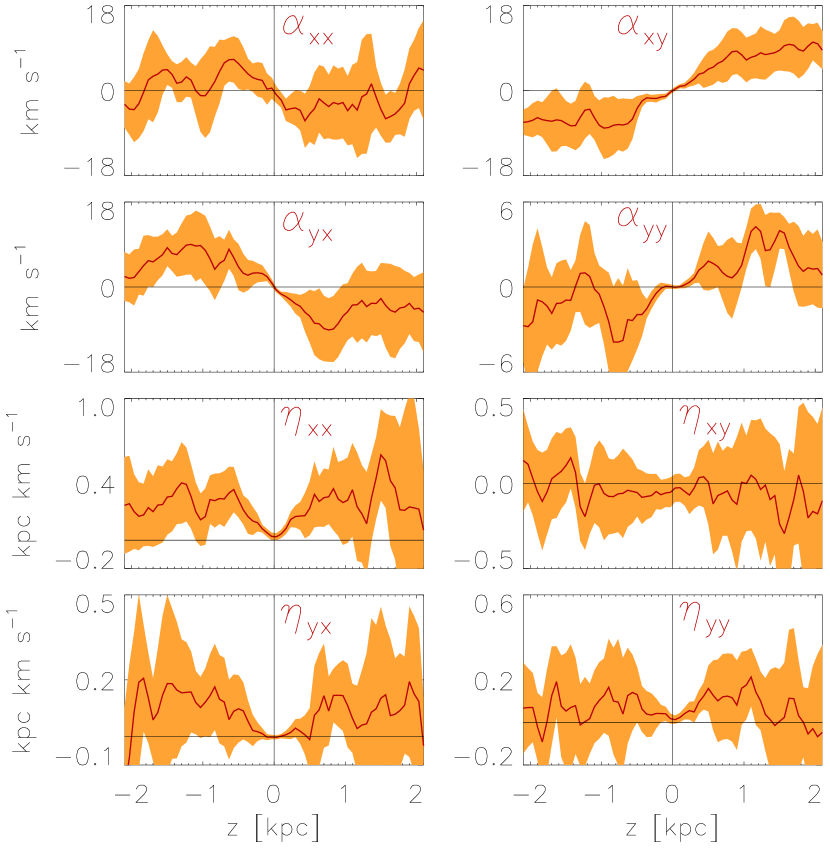
Figure 14: Same as Fig.  2 and Fig.  13, but showing results for the local regression method of BS02. Shaded regions indicate the standard variations of the coefficients when considering five separate sub-intervals in time.

As mentioned, we apply this method to the same raw data as is used for the SVD. The only difference is that the detrending in time was done by normalising with the instantaneous value of the horizontal field, $B_{\rm rms}(t)\equiv\sqrt{L_{z}^{-1}\,\int{\rm d}z\big{(}B_{x}^{2}(z,t)+B_{y}^{2}(z,t)\big{)}}$ , rather than by subtracting an exponential growth factor, as was done for SVD. As mentioned before, the purpose of the detrending is to make sure that all data are contributing in a roughly similar manner, and small changes in the procedure were not found to have a significant impact.

Unsurprisingly, the results via the regression method, shown in Fig.  14, agree markedly well with those derived via the SVD method (see Fig.  2). The standard deviation is however somewhat larger than that obtained in the SVD analysis using 9 independent time series (see Fig.  1).

References

- Beck (2012) Beck R., 2012, Space Science Reviews, 166, 215
- Beck & Wielebinski (2013) Beck R., Wielebinski R., 2013, Magnetic Fields in Galaxies. Springer Berlin Heidelberg, p. 641, doi:10.1007/978-94-007-5612-0_13
- Beck et al. (1996) Beck R., Brandenburg A., Moss D., Shukurov A., Sokoloff D., 1996, Annual Review of Astronomy and Astrophysics, 34, 155
- Bendre (2016) Bendre A. B., 2016, doctoralthesis, Universität Potsdam
- Bendre et al. (2015) Bendre A., Gressel O., Elstner D., 2015, Astronomische Nachrichten, 336, 991
- Bhat et al. (2019) Bhat P., Subramanian K., Brandenburg A., 2019, arXiv e-prints, p. arXiv:1905.08278
- Brandenburg (2005) Brandenburg A., 2005, Astronomische Nachrichten, 326, 787
- Brandenburg (2009) Brandenburg A., 2009, Space Science Reviews, 144, 87
- Brandenburg (2018) Brandenburg A., 2018, Journal of Plasma Physics, 84, 735840404
- Brandenburg & Sokoloff (2002) Brandenburg A., Sokoloff D., 2002, Geophysical & Astrophysical Fluid Dynamics, 96, 319
- Brandenburg & Subramanian (2005) Brandenburg A., Subramanian K., 2005, Physics Reports, 417, 1
- Cattaneo & Hughes (1996) Cattaneo F., Hughes D. W., 1996, Physical Review E, 54, 4532
- Enßlin (2019) Enßlin T. A., 2019, Annalen der Physik, 531, 1800127
- Fletcher (2010) Fletcher A., 2010, in Kothes R., Landecker T. L., Willis A. G., eds, Astronomical Society of the Pacific Conference Series Vol. 438, The Dynamic Interstellar Medium: A Celebration of the Canadian Galactic Plane Survey. p. 197 (arXiv:1104.2427)
- Gent et al. (2013) Gent F. A., Shukurov A., Sarson G. R., Fletcher A., Mantere M. J., 2013, MNRAS, 430, L40
- Gressel & Pessah (2015) Gressel O., Pessah M. E., 2015, ApJ, 810, 59
- Gressel et al. (2008) Gressel O., Elstner D., Ziegler U., Rüdiger G., 2008, Astronomy and Astrophysics, 486, L35
- Gressel et al. (2013) Gressel O., Bendre A., Elstner D., 2013, MNRAS, 429, 967
- Käpylä et al. (2009) Käpylä P. J., Korpi M. J., Brandenburg A., 2009, Astronomy and Astrophysics, 500, 633
- Kowal et al. (2006) Kowal G., Otmianowska-Mazur K., Hanasz M., 2006, A&A, 445, 915
- Krause et al. (2018) Krause M., et al., 2018, Astronomy & Astrophysics, 611, A72
- Kuijken & Gilmore (1989a) Kuijken K., Gilmore G., 1989a, MNRAS, 239, 571
- Kuijken & Gilmore (1989b) Kuijken K., Gilmore G., 1989b, MNRAS, 239, 605
- Kuijken & Gilmore (1989c) Kuijken K., Gilmore G., 1989c, MNRAS, 239, 651
- Mandel (1982) Mandel J., 1982, The American Statistician, 36, 15
- Moffatt (1978) Moffatt H. K., 1978, Magnetic Field Generation in Electrically Conducting Fluids. Cambridge University Press, Cambridge
- Press et al. (1992) Press W. H., Teukolsky S. A., Vetterling W. T., Flannery B. P., 1992, Numerical Recipes in C (2Nd Ed.): The Art of Scientific Computing. Cambridge University Press, New York, NY, USA
- Racine et al. (2011) Racine É., Charbonneau P., Ghizaru M., Bouchat A., Smolarkiewicz P. K., 2011, The Astrophysical Journal, 735, 46
- Rädler (1969) Rädler K.-H., 1969, Veroeffentlichungen der Geod. Geophys, 13, 131
- Rädler (2014) Rädler K. H., 2014, arXiv e-prints, p. arXiv:1402.6557
- Sánchez-Salcedo et al. (2002) Sánchez-Salcedo F. J., Vázquez-Semadeni E., Gazol A., 2002, ApJ, 577, 768
- Schrinner et al. (2005) Schrinner M., Rädler K.-H., Schmitt D., Rheinhardt M., Christensen U., 2005, Astronomische Nachrichten, 326, 245
- Schrinner et al. (2007) Schrinner M., Rädler K.-H., Schmitt D., Rheinhardt M., Christensen U. R., 2007, Geophysical and Astrophysical Fluid Dynamics, 101, 81
- Shukurov (2004) Shukurov A., 2004, arXiv e-prints, pp astro–ph/0411739
- Shukurov (2005) Shukurov A., 2005, Mesoscale Magnetic Structures in Spiral Galaxies. Springer Berlin Heidelberg, Berlin, Heidelberg, pp 113–135, doi:10.1007/3540313966_6, https://doi.org/10.1007/3540313966_6
- Simard et al. (2016) Simard C., Charbonneau P., Dubé C., 2016, Advances in Space Research, 58, 1522
- Sur et al. (2007) Sur S., Subramanian K., Brandenburg A., 2007, Monthly Notices of the Royal Astronomical Society, 376, 1238
- Tobias & Cattaneo (2013) Tobias S. M., Cattaneo F., 2013, Journal of Fluid Mechanics, 717, 347
- Warnecke et al. (2016) Warnecke J., Rheinhardt M., Tuomisto S., Käpylä P. J., Käpylä M. J., Brandenburg A., 2016, preprint, (arXiv:1601.03730)
- Ziegler (2008) Ziegler U., 2008, Computer Physics Communications, 179, 227