Poisson Noise Removal Using Multi-Frame 3D Block Matching

Abstract

The 3D block matching (BM3D) filter belongs to the state-of-the-art techniques for eliminating additive white Gaussian noise from single-frame images. There exist four multi-frame extensions of BM3D as of today. In this work, we combine these extensions with a variance stabilising transformation (VST) for eliminating Poisson noise. Our evaluation reveals that the extension which retains the original noise model of the noisy images and additionally has a comprehensive connectivity of 2D and temporal image information at both pixel and patch levels, gives the best results. Additionally, we find a surprising change in performance of one the four extensions due to the specific application of the VST. Finally, we also introduce a simple low-pass filtering as a preprocessing step for the best performing extension. This can give rise to a significant additional improvement of 0.94 dB in the output according to the peak signal to noise ratio.

Index Terms—  Multi-frame denoising, non-local patch methods, Poisson noise, 3D block matching

1 Introduction

Image acquisition through CCD/CMOS sensors is dominated by Poisson noise distribution [1]. Astronomical imaging [2], medical imaging [3], and electron microscopy [4] are some of the specific applications where we encounter Poisson noise. There are two categories of imaging techniques that are designed to eliminate Poisson noise: In one of the categories, additive white Gaussian noise (AWGN) elimination algorithms [5, 6, 7, 8, 9] are combined with variance stabilising transformations (VST) [10, 11, 12]. The other category comprises of algorithms that are designed for eliminating Poisson noise directly [13, 14, 15]. Among all these techniques, 3D block matching (BM3D) [5] when combined with a VST, gives the best denoising results in most cases [11].

All the above mentioned techniques concentrate on denoising single-frame images. There has not been much investigation in the field of multi-frame image denoising. In applications such as electron microscopy, CT imaging and multi-spectral imaging, we encounter situations where multiple images of the same scene can be acquired. Further processing is required for fusing the information from all the images to one single image. Several approaches [16, 17, 18, 19, 20, 21, 22, 23, 24, 25] that have been designed to remove both AWGN and Poisson noise from multi-frame image datasets, are inspired from algorithms that are originally designed for single-frame image denoising.

Non-local patch-based methods [5, 26, 27] are among the best performing methods for single-frame image denoising. Efforts in the direction of optimally extending non-local patch based methods to multi-frame elimination of signal dependent noise [20, 22], made use a of hybrid filtering scheme. In particular, depending on the temporal standard deviation after registration, they use a combination of values computed through simple averaging of the frames and primitive spatio-temporal non-local patch-based methods. We have revived the research in this direction in [28], by studying all possible spatio-temporal extensions of 3D block matching in the multi-frame scenario. In particular, we have evaluated our proposed extensions and existing ones for eliminating AWGN. We have learnt from this evaluation that using multi-frame extension ideas which retain the noise model and simultaneously enhance the connectivity between frames, give superior results. The optimal performance of such ideas in the AWGN layout, motivates us to also analyse their capability in the multi-frame Poisson noise scenario.

Our Contribution. There exist four extensions of BM3D for multi-frame AWGN removal [28]. In the present work, we perform a comparative evaluation of these extensions for eliminating Poisson noise from multi-frame image datasets. For this purpose, we combine all four extensions with the Anscombe transform and the closed-form approximation of the exact unbiased inverse Anscombe transform. The difference in the qualitative performance according to peak-signal-to-noise (PSNR) ratio, between the closed-form approximation and the exact unbiased inverse is small, but the former is faster [12]. Hence, we use the closed-form approximation for computing the inverse variance stabilising transformation. Additionally, we introduce a preprocessing step for the best performing extension after the evaluation, in the form of simple low-pass filtering. This extra step significantly improves the denoising output.

Paper Structure. In Section 2, we introduce our novel framework that uses various extensions of BM3D for eliminating Poisson noise from multi-frame image datasets. In Section 3, we present our experimental results. We also provide explanations behind the respective positions of different extensions in the ranking. Finally, in Section 4, we present a summary of our work and give an outlook to future work.

2 Modelling of denoising algorithm

There are two trivial and two non-trivial extensions among the four existing extensions of BM3D for multi-frame AWGN removal [28]. In Sections 2.1 and 2.2 we review these four extensions. In Sections 2.3 and 2.4 we explain in detail the exact procedure that makes optimal use of these four extensions for multi-frame Poisson noise elimination.

2.1 Trivial Extensions of BM3D

BM3D-1: In the first trivial extension [28], we first average all the frames after registering them. In the second step, we use the original BM3D method [5] to denoise the averaged image.

BM3D-2: In the second trivial extension [28], we first denoise every single frame using the original BM3D method. In the second step, we average all the denoised frames after registering them.

Image	BM-1	BM-2	BM-3	BM-M	$\sigma$/ BM-Mσ
House (1)	18.29	22.73	22.94	24.28	95/ 24.74
House (2)	21.19	26.02	25.53	27.11	100/ 27.28
House (3)	23.15	27.29	26.49	28.13	110/ 28.32
House (4)	24.69	28.14	27.23	29.06	105/ 29.32
House (5)	25.97	28.87	27.91	29.74	120/ 29.92
Lena (1)	19.00	24.54	23.90	25.33	195/ 25.88
Lena (2)	21.64	26.53	25.82	27.31	200/ 27.50
Lena (3)	23.43	27.67	26.77	28.44	220/ 28.62
Lena (4)	24.84	28.33	27.41	29.13	215/ 29.24
Lena (5)	25.86	28.94	27.95	29.67	210/ 29.82
Bridge (1)	18.02	20.79	20.40	21.16	130/ 21.85
Bridge (2)	19.85	21.93	21.50	22.36	145/ 22.88
Bridge (3)	20.95	22.59	22.08	23.08	140/ 23.55
Bridge (4)	21.73	23.04	22.48	23.55	145/ 24.00
Bridge (5)	22.26	23.38	22.80	23.89	145/ 24.33
Peppers (1)	20.48	24.75	23.97	25.53	170/ 26.10
Peppers (2)	22.78	26.68	25.83	27.46	195/ 27.63
Peppers (3)	24.49	27.69	26.77	28.41	205/ 28.54
Peppers (4)	25.64	28.42	27.48	29.14	205/ 29.24
Peppers (5)	26.50	28.89	27.94	29.57	205/ 29.67

BM-1	BM-2	BM-3	BM-M	$\sigma$/ BM-Mσ
17.55	22.98	23.34	25.20	80/ 26.11
20.51	26.41	25.79	27.93	90/ 28.26
22.67	27.77	26.73	29.26	105/ 29.58
24.25	28.60	27.55	30.09	100/ 30.48
25.60	29.28	28.23	30.73	100/ 31.06
18.16	24.78	24.12	25.95	165/ 26.91
20.98	26.92	26.07	28.24	180/ 28.71
22.92	28.05	26.99	29.41	195/ 29.75
24.42	28.75	27.64	30.13	195/ 30.42
25.55	29.28	28.08	30.64	195/ 30.94
17.41	20.90	20.53	21.46	115/ 22.53
19.49	22.10	21.64	22.86	130/ 23.66
20.77	22.72	22.18	23.61	135/ 24.32
21.62	23.20	22.61	24.19	145/ 24.81
22.23	23.55	22.90	24.57	145/ 25.15
19.65	24.99	24.20	26.22	160/ 27.07
22.16	26.99	26.09	28.30	175/ 28.71
23.99	28.02	26.95	29.31	180/ 29.60
25.23	28.78	27.65	30.03	175/ 30.25
26.14	29.24	28.12	30.47	185/ 30.69

Table 1: PSNR values after denoising 5-image (left) and 10-image (right) datasets with noise peaks varying from 1 to 5.

2.2 Non-Trivial Extensions of BM3D

BM3D-3: The original BM3D method is a two-step process. Initially, for every reference patch considered, a corresponding 3D group of patches is formed by searching for the most similar patches in the image with respect to the $L_{2}$ distance. In the first non-trivial extension BM3D-3 [29, 21, 20, 22], we consider a reference frame initially. For every reference patch in this frame we increase the search area for finding the most similar patches from this particular frame to all the frames. The further procedure is similar to the original BM3D method.

BM3D-4: The second non-trivial extension [28] is also a two-step method with three sub-steps in each step like the original BM3D method:
Step 1.1 - Grouping. Unlike BM3D-3, here we consider reference patches from all the frames but not just one frame. A corresponding 3D group for every reference patch is then created by finding the most similar patches in all the frames using $L_{2}$ distance. We remove the threshold parameters for $L_{2}$ distance. This is done because there is a risk of losing similar patches for high amplitudes of noise. However, we retain the parameters that specify the maximum number of patches in a 3D group.
Step 1.2 - Filtering. We apply the following techniques on every obtained 3D group, in the same order: 2D bi-orthogonal spline wavelet transform, 1D Walsh-Hadamard transform, hard thresholding, 1D Walsh-Hardamard back transform, and a 2D bi-orthogonal spline wavelet back transform.
Step 1.3 - Aggregation. Now, every pixel in every frame is denoised at least once after the second sub-step. The denoised versions of every pixel is present in 3D groups belonging to the frame the pixel belongs to, as well as in 3D groups from other frames. Thus, we first compute a weighted aggregation of all the denoised versions of every pixel within the frame in which it is present. This gives us as many initial denoised frames as there are input frames. To compute a final denoised frame after the first main step, we use the following equation for weighted aggregation across 3D groups in all frames:

$$\bm{u}^{\textrm{{basic}}}({\bm{x}})=\frac{\sum\limits_{\ell}\sum\limits_{P_{\ell}}w_{P_{\ell}}^{\textrm{{hard}}}\sum\limits_{Q\in P(\textrm{P}_{\ell})}\chi_{Q}(\bm{x})\bm{u}^{\textrm{{hard}}}_{Q,P_{\ell}}(\bm{x})}{\sum\limits_{l}\sum\limits_{P_{\ell}}w_{P_{\ell}}^{\textrm{{hard}}}\sum\limits_{Q\in P(\textrm{P}_{\ell})}\chi_{Q}(\bm{x})}.$$ (1)

Here, $\bm{x}$ is a position in the 2D image domain $Q$ and $\bm{u}^{\textrm{{basic}}}$ is the initial denoised image. The set of most similar patches to the reference patch $P_{\ell}$ belonging to frame $\ell$, are denoted using $\mathcal{P}(P_{\ell})$. We have $\chi_{Q}(\bm{x})=1$ if $\bm{x}\in Q$ and 0 otherwise, for every patch $Q$ in the set $\mathcal{P}(P_{\ell})$. The symbol $\bm{u}^{\textrm{{hard}}}_{Q,P_{\ell}}(\bm{x})$ denotes the estimation of the value at pixel position $\bm{x}$, belonging to the patch $Q$, derived after the hard thresholding (with coefficients $w_{P_{\ell}}^{\textrm{{hard}}}$) of the reference patch $P_{\ell}$.
Step 2.1 - Grouping. The same grouping strategy as in 1.1 is employed by us, using the reference patches from the initial denoised frames computed after the first main step.
Step 2.2 - Filtering. We execute the following techniques on every obtained 3D group and the corresponding initial noisy 3D group, in the same order: 2D discrete cosine transform, 1D Walsh-Hadamard transform, Wiener filtering on a combination of both the corresponding 3D groups, 1D Walsh-Hadamard back transform, and a 2D discrete cosine back transform.
Step 2.3 - Aggregation. The same corresponding strategy as in 1.3 is exploited by us to estimate the final denoised image. This aggregation strategy can be represented as:

$$\bm{u}^{\textrm{{final}}}({\bm{x}})=\frac{\sum\limits_{\ell}\sum\limits_{P_{\ell}}w_{P_{\ell}}^{\textrm{{wien}}}\sum\limits_{Q\in P(\textrm{P}_{\ell})}\chi_{Q}(\bm{x})\bm{u}^{\textrm{{wien}}}_{Q,P_{\ell}}(\bm{x})}{\sum\limits_{l}\sum\limits_{P_{\ell}}w_{P_{\ell}}^{\textrm{{wien}}}\sum\limits_{Q\in P(\textrm{P}_{\ell})}\chi_{Q}(\bm{x})}.$$ (2)

Here wien represents Wiener filtering and $\bm{u}^{\textrm{{final}}}$ is the final denoised image. The rest of the symbols have the same meaning as in (1). Moreover, we can also represent the initial denoised image aggregated using BM3D-3 by (1). Choosing $\ell=1$ in (1) gives us the initial estimate of the single-frame BM3D algorithm. The final denoised image using BM3D-3 and single-frame BM3D can both be computed by selecting $\ell=1$ in (2).

We apply the particular filtering steps 1.2 and 2.2 in the Fourier domain because of better differentiation between signal and noise when compared to the Cartesian domain. The original work [5] provides more specific details regarding the single-frame BM3D algorithm.

In the first extension, we have a change in the noise distribution because of averaging the noisy frames. In BM3D-2, we denoise every frame first, which is a sub-optimal solution since we have limited amount of signal in each of the frames. BM3D-3 avoids the above two modelling disadvantages by searching for similar patches in all the frames. However, we consider just one reference frame and this does not allow us to make use of the complete information. In the final extension BM3D-4, we consider every frame as the reference frame. This allows us to compute similar patches from all the frames in both the main steps, unlike BM3D-3. Such a modelling also allows us to perform a better aggregation for obtaining the final denoised image. This is due to the presence of more denoised versions of every pixel in the 2D image domain, when compared to the third extension.

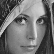
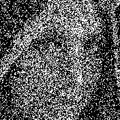
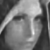
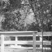
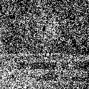
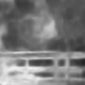
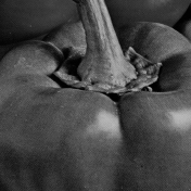
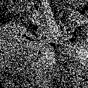
Fig. 1: Results after denoising 5-image datasets with noise peak of 1.0. Top to bottom: Zoom into the Lena, House, Bridge, Peppers images. Left to right: Original, noisy, BM3D-4_σ, next best method.

2.3 Denoising with Variance Stabilisation

We carry out the following procedure for eliminating Poisson noise by using the various BM3D extensions mentioned above: All the noisy datasets undergo the Anscombe transformation for variance stabilisation, affine rescaling to [0,1] greyscale range, filtering using one of the four extensions, affine rescaling back to the original range, and finally the closed-form approximation of the exact unbiased inverse Anscombe transformation.

In BM3D-1, we have applied the transformation on the averaged image while in all other extensions we have applied the VST directly on the initial noisy images. One can find more details regarding the above general procedure and parameter selection in [11, 12, 30].

2.4 Low-Pass Filtering

As already mentioned in Section 1, we use a simple low pass filter [31] as a preprocessing step for the best performing extension. The following low-pass filter is applied on the noisy images directly (without variance stabilisation or affine rescaling), in order to make the process of finding similar patches that form a 3D group more robust:

$$H(\bm{\hat{x}})=\begin{cases}1&\text{$\textrm{for}\ \ |\bm{\hat{x}}|<\frac{\sigma}{2}$},\\ \textrm{exp}\left(\frac{-(\hat{x}-(\frac{\sigma}{2}))^{2}-(\hat{y}-(\frac{\sigma}{2}))^{2}}{2(\frac{\sigma}{2})^{2}}\right)&\textrm{for}\ \ |\bm{\hat{x}}|\geq\frac{\sigma}{2}.\end{cases}$$

Here, $\bm{\hat{x}}:=(\hat{x},\hat{y})^{\top}$ represents the 2D frequency vector in the Fourier domain and $\sigma$ specifies the shape of the filter. The Gaussian-type decay of the filter coefficients is intended to reduce the transform-domain filtering artifacts. We use the low-pass filtered image only for forming the 3D groups in the first main step and nowhere else in the entire algorithm.

3 Experiments and Discussion

In multi-frame denoising applications, the frames are first registered using motion registration algorithms before denoising them. In this work we want to specifically test the denoising capability of different extensions of BM3D. To this end, we assume that the frames are perfectly registered similar to [28]. This assumption makes even more sense because it has already been verified [20, 22] that denoising methods (even without temporal support) are superior to averaging at regions where there is high temporal standard deviation after registration. Thus, verifying the performance of different denoising methods assuming perfect registration also covers the remaining case of less temporal standard deviation. Thereby, to create this experimental setting, we have added Poisson noise to the Lena, House, Peppers and Bridge images with noise peaks varying from 1 to 5. Due to the signal dependent nature of Poisson noise, we have high noise amplitude when the intensity of the signal decreases. The noise peak value controls this trade-off. Lesser noise peak value indicates higher amount of noise. For every image and every noise peak, we have created two datasets each with 5 and 10 realisations of noise.

Dissolving the threshold parameters for $L_{2}$ distance while forming the 3D groups is advantageous to all the extensions. Hence, we have excluded this parameter in both the main steps of BM3D for all the four extensions.

For BM3D-3, in the results which we showcase shortly, we present the best PSNR after every frame is considered as the reference frame.

From Table 1 and Figure 1, we can conclude that both visually and in terms of PSNR, the non-trivial extension BM3D-4 outperforms all other extensions significantly. The comprehensive inter-frame connectivity strategy used in BM3D-4 is the reason behind its significantly better performance. Also, using a low-pass filter for preprocessing (BM3D-4_σ) gives BM3D-4 a noteworthy improvement (0.94 dB for the Lena 10-image dataset).

There can be imprecision in variance stabilisation when the VST is applied on a single noisy image [32]. The imprecision is even higher because of the initial averaging step in BM3D-1, which modifies the noise distribution. This is clearly evident from Table 1 because denoising 5 images is surprisingly better than denoising 10 images using BM3D-1. We can avoid such a problem using BM3D-4 as it does not average the initial noisy images but retains the original noise model.

BM3D-4 is slightly more than $2L$ times (two main steps and the extensive patch-matching) slower than single-frame BM3D, for a dataset with $L$ frames. Our CUDA implementation of BM3D-4 on an NVIDIA GeForce GTX 1070 device takes 1.76 seconds for a dataset sized $256\times 256\times 5$.

4 Conclusions and Outlook

In this work we have evaluated the capability of different existing extensions of BM3D to remove multi-frame Poisson noise, by combining them with a variance stabilising tranformation. Our evaluation revealed that the extension (BM3D-4) which retains the original noise model and additionally makes use of the complete available information through a comprehensive connectivity of 2D and temporal information, is the best method for multi-frame Poisson noise elimination. Our new idea to preprocess the data using low-pass filtering gives significant additional quality improvement to the best performing extension BM3D-4.

In the future, we will explore the application of BM3D-4 for eliminating Poisson and Poisson-Gaussian mixture noise of varying amplitudes in the same dataset. We also plan to use BM3D-4 for denoising datasets acquired with electron microscopes, by combining it with state-of-the-art motion registration algorithms.

Acknowledgements. J.W. has received funding from the European Research Council (ERC) under the European Union’s Horizon 2020 research and innovation programme (grant agreement no. 741215, ERC Advanced Grant INCOVID).

References

- [1] F. Rooms, W. Philips, and P. Van Oostveldt, “Integrated approach for estimation and restoration of photon-limited images based on steerable pyramids,” in Proc. 2003 EURASIP Conference Focussed on Video/Image Processing and Multimedia Communications, Zagreb, Croatia, July 2003, pp. 131–136, IEEE.
- [2] K. J. Borkowski, S. P. Reynolds, D. A. Green, U. Hwang, and R. Petre, “Radioactive scandium in the youngest galactic supernova remnant G1.9+0.3,” The Astrophysical Journal Letters, vol. 724, no. 2, pp. L161, Nov. 2010.
- [3] I. Rodrigues, J. Sanches, and J. Bioucas-Dias, “Denoising of medical images corrupted by Poisson noise,” in Proc. 2008 IEEE International Conference on Image Processing, San Diego, CA, USA, Oct. 2008, pp. 1756–1759.
- [4] J.R. Jinschek, K.J. Batenburg, H.A. Calderon, R. Kilaas, V. Radmilovic, and C. Kisielowski, “3D reconstruction of the atomic positions in a simulated gold nanocrystal based on discrete tomography: Prospects of atomic resolution electron tomography,” Ultramicroscopy, vol. 108, no. 6, pp. 589–604, May 2008.
- [5] K. Dabov, A. Foi, V. Katkovnik, and K. Egiazarian, “Image denoising by sparse 3D transform-domain collaborative filtering,” IEEE Transactions on Image Processing, vol. 16, no. 8, pp. 2080–2095, Aug. 2007.
- [6] J. Boulanger, J. B. Sibarita, C. Kervrann, and P. Bouthemy, “Non-parametric regression for patch-based fluorescence microscopy image sequence denoising,” in Proc. 2008 IEEE International Symposium on Biomedical Imaging: From Nano to Macro, Paris, France, May 2008, pp. 748–751.
- [7] B. Zhang, J. M. Fadili, and J. L. Starck, “Wavelets, ridgelets, and curvelets for Poisson noise removal,” IEEE Transactions on Image Processing, vol. 17, no. 7, pp. 1093–1108, July 2008.
- [8] P. Fryzlewicz and G. P. Nason, “A Haar-Fisz algorithm for Poisson intensity estimation,” Journal of Computational and Graphical Statistics, vol. 13, no. 3, pp. 621–638, Jan. 2012.
- [9] J. Portilla, V. Strela, M. J. Wainwright, and E. P. Simoncelli, “Image denoising using scale mixtures of Gaussians in the wavelet domain,” IEEE Transactions on Image Processing, vol. 12, no. 11, pp. 1338–1351, Nov. 2003.
- [10] F. J. Anscombe, “The transformation of Poisson, binomial and negative-binomial data,” Biometrika, vol. 35, no. 3/4, pp. 246–254, Dec. 1948.
- [11] M. Mäkitalo and A. Foi, “Optimal inversion of the Anscombe transformation in low-count Poisson image denoising,” IEEE Transactions on Image Processing, vol. 20, no. 1, pp. 99–109, Jan. 2011.
- [12] M. Mäkitalo and A. Foi, “A closed-form approximation of the exact unbiased inverse of the Anscombe variance-stabilizing transformation,” IEEE Transactions on Image Processing, vol. 20, no. 9, pp. 2697–2698, Sept. 2011.
- [13] S. Lefkimmiatis, P. Maragos, and G. Papandreou, “Bayesian inference on multiscale models for Poisson intensity estimation: Applications to photon-limited image denoising,” IEEE Transactions on Image Processing, vol. 18, no. 8, pp. 1724–1741, Aug. 2009.
- [14] F. Luisier, C. Vonesch, T. Blu, and M. Unser, “Fast interscale wavelet denoising of Poisson-corrupted images,” Signal Processing, vol. 90, no. 2, pp. 415–427, Feb. 2010.
- [15] R. M. Willett and R. D. Nowak, “Platelets: a multiscale approach for recovering edges and surfaces in photon-limited medical imaging,” IEEE Transactions on Medical Imaging, vol. 22, no. 3, pp. 332–350, Mar. 2003.
- [16] T. Blu and F. Luisier, “The SURE-LET approach to image denoising,” IEEE Transactions on Image Processing, vol. 16, no. 11, pp. 2778–2786, Nov. 2007.
- [17] A. M. Hasan, A. Melli, K. A. Wahid, and P. Babyn, “Denoising low-dose CT images using multi-frame blind source separation and block matching filter,” IEEE Transactions on Radiation and Plasma Medical Sciences, vol. 2, no. 4, pp. 279–287, July 2018.
- [18] J. Boulanger, C. Kervrann, P. Bouthemy, P. Elbau, J. B. Sibarita, and J. Salamero, “Patch-based nonlocal functional for denoising fluorescence microscopy image sequences,” IEEE Transactions on Medical Imaging, vol. 29, no. 2, pp. 442–454, Feb. 2010.
- [19] W. Dong, G. Li, G. Shi, X. Li, and Y. Ma, “Low-rank tensor approximation with Laplacian scale mixture modeling for multiframe image denoising,” in Proc. 2015 IEEE International Conference on Computer Vision, Santiago, Chile, Dec. 2015, pp. 442–449.
- [20] T. Buades, Y. Lou, J. M. Morel, and Z. Tang, “A note on multi-image denoising,” in Proc. 2009 IEEE International Workshop on Local and Non-Local Approximation in Image Processing, Tuusula, Finland, Oct. 2009, pp. 1–15.
- [21] M. Tico, “Multi-frame image denoising and stabilization,” in Proc. 2008 IEEE European Signal Processing Conference, Lausanne, Switzerland, Aug. 2008, pp. 1–4.
- [22] A. Buades, Y. Lou, J. M. Morel, and Z. Tang, “Multi Image Noise Estimation and Denoising,” HAL Archives, hal-00510866, version 1, Aug. 2010.
- [23] L. Fang, S. Li, Q. Nie, J. A. Izatt, C. A. Toth, and S. Farsiu, “Sparsity based denoising of spectral domain optical coherence tomography images,” Biomedical Optics Express, vol. 3, no. 5, pp. 927–942, 2012.
- [24] F. Luisier, C. Vonesch, T. Blu, and M. Unser, “Fast Haar-wavelet denoising of multidimensional fluorescence microscopy data,” in Proc. 2009 IEEE International Symposium on Biomedical Imaging: From Nano to Macro, Boston, MA, USA, July 2009, pp. 310–313.
- [25] L. Zhang, S. Vaddadi, H. Jin, and S. K. Nayar, “Multiple view image denoising,” in Proc. 2009 IEEE Conference on Computer Vision and Pattern Recognition, Miami, FL, USA, June 2009, pp. 1542–1549.
- [26] M. Lebrun, A. Buades, and J.M. Morel, “A nonlocal Bayesian image denoising algorithm,” SIAM Journal on Imaging Sciences, vol. 6, no. 3, pp. 1665–1688, Sept. 2013.
- [27] M. Lebrun, “An analysis and implementation of the BM3D image denoising method,” Image Processing On Line, vol. 2, pp. 175–213, Aug. 2012.
- [28] K. Bodduna and J. Weickert, “Enhancing patch-based methods with inter-frame connectivity for denoising multi-frame images,” in Proc. 2019 IEEE International Conference on Image Processing (To appear), Taipei, Taiwan, Sept. 2019.
- [29] A. Buades, B. Coll, and J. Morel, “Denoising image sequences does not require motion estimation,” in Proc. 2005 IEEE Conference on Advanced Video and Signal Based Surveillance, Como, Italy, Sept. 2005, pp. 70–74.
- [30] Y. Hou, C. Zhao, D. Yang, and Y. Cheng, “Comments on ”Image denoising by sparse 3D transform-domain collaborative filtering”,” IEEE Transactions on Image Processing, vol. 20, no. 1, pp. 268–270, Jan. 2011.
- [31] A. Frangakis and R. Hegerl, “Noise reduction in electron tomographic reconstructions using nonlinear anisotropic diffusion,” Journal of Structural Biology, vol. 135, no. 3, pp. 239–250, Sept. 2001.
- [32] L. Azzari and A. Foi, “Variance stabilization for noisy+estimate combination in iterative Poisson denoising,” IEEE Signal Processing Letters, vol. 23, no. 8, pp. 1086–1090, Aug. 2016.