SINR Analysis of Different Multicarrier Waveforms over Doubly Dispersive Channels

Abstract

Wireless channels generally exhibit dispersion in both time and frequency domain, known as doubly selective or doubly dispersive channels. To combat the delay spread effect, multicarrier modulation (MCM) such as orthogonal frequency division multiplexing (OFDM) and its universal filtered variant (UF-OFDM) is employed, leading to the simple per-subcarrier one tap equalization. The time-varying nature of the channel, in particular, the intra-multicarrier-symbol channel variation induces spectral broadening and thus inter-carrier interference (ICI). Existing works address both effects separately, focus on the one effect while ignoring the respective other. This paper considers both effect simultaneously for cyclic prefix (CP)-, zero padded (ZP)- and UF-based OFDM with simple one tap equalization, assuming a general wireless channel model. For this general channel model, we show that the independent (wide sense stationary uncorrelated scatter, WSSUS) selectivity in time and frequency starts to intertwine in contrast to the ideal cases with single selectivity. We derive signal-to-interference-plus-noise ratio (SINR) in closed form for arbitrary system settings and channel parameters, e.g., bandwidth, delay- and Doppler-spread. With the SINR analysis, we compare the three MCM schemes under different channel scenarios.

I Introduction

Multicarrier modulation (MCM), particularly orthogonal frequency division multiplexing (OFDM), is proven to be the most practical technique in terms of spectral efficiency and transceiver complexity. Relying on orthogonal subcarriers with lower data rate, the channel-induced inter-symbol interference (ISI) is significantly suppressed in comparison to single carrier systems. With the help of a cyclic prefix (CP) and/or zero padding (ZP) [1], though sacrificing some spectral efficiency, ISI can be completely mitigated in OFDM so that the equalization procedure is drastically simplified to a single tap.

The orthogonality between OFDM subcarriers is often questioned in practical systems because of nonlinear impairments of RF components such as power amplifier and inaccurate transmit and receive oscillators. This is even more critical in OFDMA scenarios, i.e., multi-user uplink transmissions, where each user has its own RF chain making the maintenance of orthogonality much more demanding. To improve the spectral properties of OFDM, thus reduce inter-carrier interference (ICI) in the absence of orthogonality, a subband-based filtering approach was proposed and studied in [2, 3, 4, 5, 6, 7, 8, 9, 10, 11, 12, 13, 14], termed universal filtered OFDM (UF-OFDM). The redundant cyclic prefix in OFDM, which serves as guard time between symbols, is devoted to FIR-filtering [15, 16, 17] of a subband in UF-OFDM as the consequence of the Balian–Low theorem prohibiting good per-subcarrier spectral shaping with short filter (comparable to CP/ZP, e.g., $8\%-15\%$ of symbol length).

The trend of future communication systems is to be more heterogeneous, support faster vehicles and operate at higher carrier frequencies. The often ignored intra OFDM symbol channel variation, i.e., time selectivity, starts to play a role. In [18][19], the effect and/or bound of Doppler spread with Jakes, uniform and two path model is analyzed. The equalization of Doppler spread in the context of OFDM is studied in [20][21] and [22]. However, all the existing literature assume CP/ZP length larger than the maximum channel delay spread so that frequency selectivity has no impact on the Doppler-induced ICI. As pointed out in [23], frequency-selectivity of the channel has only moderate impact on the performance. Therefore, it is often neglected in the vast majority of works. To the best of the authors’ knowledge, a comprehensive study of ICI and inter-symbol interference (ISI) in general cases of MCM parameters and channel statistics has not yet been done. Although the channel fading in time and frequency is believed to be independent of each other, the interplay complicates the ICI and ISI analysis if the channel delay spread is not restricted to within CP/ZP duration.

This paper addresses both time- and frequency-selectivity of general wireless channels. Both ICI and ISI are analytically computed using derived closed-form formulas assuming the low-complexity single tap equalization. Both, time and frequency correlation functions, are incorporated in the analytical formula, covering all cases of CP/ZP lengths, channel delay spreads and Doppler spreads. We compare the SINR performance of the classic CP- and ZP-OFDM with the novel UF-OFDM in both uplink (multiuser with diverse selectivity parameters) and downlink (multiuser with same selectivity parameters) settings. The analysis reveals that CP- and ZP-OFDM is robust to delay spread and UF-OFDM is robust to Doppler spread, which provides guideline for waveform choice depending on application-constrained channel statistics.

Notation: We use $\left(\cdot\right)^{H}$ to denote Hermitian transpose, $\mathrm{diag}\left(\cdot\right)$ diagonal elements vector of matrices and/or diagonal matrices of vectors, $\mathrm{tr}\left(\cdot\right)$ the trace operator. The modulo-$N$ operation is denoted by $\left\langle\cdot\right\rangle_{N}$ and the element in the $i$th row and $j$th column of the matrix $\mathbf{A}$ is denoted by $\left[\mathbf{A}\right]_{ij}$. Occasionally, we use $\mathbf{A}_{j}$ to denote the $j$th row vector of the matrix $\mathbf{A}$ for brevity. Finally, $K$-point IDFT and DFT matrices are denoted by $\mathbf{F}_{K}^{H}$ and $\mathbf{F}_{K}$ with normalized power, respectively.

II System model and doubly selective channel

A system with a bandwidth of $N$ subcarriers is considered. A user moving at the speed of $v_{u}$ is allocated with $M$ consecutive subbands for data transmission, each consisting of $N_{\mathrm{RB}}$ subcarriers. The $m$th transmit signal $\mathbf{x}_{m}$ of the user using OFDM is expressed as

$$\mathbf{x}_{m,\mathrm{O}}=\mathbf{C}_{\mathrm{A}}\cdot{\displaystyle\sum_{i=1}^{M}}\mathbf{F}_{i}^{H}\cdot\mathbf{X}_{m,i},$$ (1)

where $\mathbf{X}_{m,i}$ with the dimension $N_{\mathrm{RB}}\times 1$ denotes the $m$th QAM symbol vector of the $i$th subband, $\mathbf{F}_{i}^{H}$ is the corresponding inverse Fourier transform matrix and $\mathbf{C}_{A}$ adds $L_{\mathrm{CP}}$ samples of cyclic (or zero) prefix after the Fourier transform.

UF-OFDM applies FIR-filtering after the Fourier transform to improve the spectral property instead of inserting cyclic prefix. To ensure the same spectral efficiency, FIR filters with the order $L=L_{\mathrm{F}}=L_{\mathrm{CP}}$ are used. Furthermore, the filtering is performed in a subband basis, i.e., the $m$th transmit symbol reads

$$\mathbf{x}_{m,\mathrm{U}}={\displaystyle\sum_{i=1}^{M}}\mathbf{G}_{i}\cdot\mathbf{F}_{i}^{H}\cdot\mathbf{X}_{m,i},$$ (2)

where $\mathbf{G}_{i}$ is a Toeplitz matrix comprising of the subband filter coefficients $[g_{i,0},\cdots,g_{i,L_{\mathrm{F}}}]$. The same type of filter with adjusted center frequency is often used for each subband.

The wireless channel is in general time and frequency selective, which results from dispersion (or broadening) in both time (multipath) and frequency (Doppler). To account for both effects, the doubly selective channel is often mathematically modeled by

$$\underset{\left[\left(N+L+D\right)\,\times\,\left(N+L\right)\right]}{\mathbf{h}_{m}}=\left[\begin{array}[]{ccccc}h_{00}&&0&&0\\ h_{10}&h_{01}\\ \vdots&h_{11}&\ddots\\ h_{D0}&\vdots&\ddots&&h_{0N+L}\\ &h_{D1}&&&h_{1N+L}\\ 0&0&\ddots&&\vdots\end{array}\right],$$ (3)

where $h_{ij}\thicksim\mathcal{CN}\left(0,\rho_{i}\right)$ is circularly symmetric complex Gaussian distributed with zero mean and variance $\rho_{i}$. It denotes the channel response of the $i$th tap at the $j$th time instance and $D$ is the memory order of the channel. Under the wide sense stationary uncorrelated scatterers (WSSUS) assumption, it holds

$$\mathrm{E}\left[h_{ij}\cdot h_{mn}^{*}\right]=\begin{cases}0&i\neq m\\ \rho_{i}R_{t}\left(\Delta n=j-n\right)&i=m\end{cases},$$ (4)

where $R_{t}\left(\Delta n\right)$ is the correlation between the channel coefficients at two different time instances. In classic Clark and Jakes model, the correlation function in time is given by

$$R_{t}\left(\Delta n\right)=J_{0}\left(2\pi f_{D}T_{s}\cdot\Delta n\right),$$ (5)

where $J_{0}\left(\cdot\right)$ is the zero-th order Bessel function of the first kind, $f_{D}$ denotes the Doppler frequency and $T_{s}$ denotes the time between two consecutive samples. Taking the Fourier transform of the correlation function which results in the famous Bathtub spectrum, the spectral broadening becomes obvious inducing ICI. The multipath propagation on the other hand causes ISI, if not properly dealt with, and frequency selectivity. An exponential power delay profile is investigated throughout this paper, i.e., $\rho_{i}=\rho_{0}\beta^{i}$, if not otherwise stated. Briefly speaking, the power of the channel impulse response decays exponentially with its delay. The frequency correlation function can be obtained by taking Fourier transform of the power delay profile (PDP), i.e.,

$$R_{f}\left(\Delta k\right)=\frac{\rho_{0}}{\sqrt{N}}\cdot\frac{1-\beta^{N}e^{j2\pi\Delta k}}{1-\beta e^{j2\pi\frac{\Delta k}{N}}}.$$ (6)

Furthermore, the mean delay spread and root mean square (rms) delay spread are given by the first moment and the standard deviation of the PDP.

III SINR analysis

For simplicity of notation, yet without loss of generalization, single subband allocation is considered (i.e., $M=1$) in the following. Let $\mathbf{x}_{m}$ denote either $\mathbf{x}_{m,\mathrm{O}}$ or $\mathbf{x}_{m,\mathrm{U}}$ with a little abuse of notation. Consider the detection of the $m$th (OFDM and/or UF-OFDM) symbol, the received signal within the detection window consists of part of the signal of interest and part of previous symbol due to the channel delay spread with the assumption $D\leq N-L$ (so that merely the previous symbol contributes to ISI), which reads

$$\mathbf{y}_{m}=\mathbf{w}_{\mathrm{D}}\mathbf{h}_{m}\mathbf{x}_{m}+\mathbf{w}_{\mathrm{I}}\mathbf{h}_{m-1}\mathbf{x}_{m-1}+\mathbf{n}$$ (7)

where $\mathbf{n}$ denotes uncorrelated Gaussian noise with $\sigma_{n}^{2}\mathbf{I}$ auto-covariance, $\mathbf{w}_{\mathrm{D}}$ and $\mathbf{w}_{\mathrm{I}}$ are to model the detection window and ISI, they can be expressed by

$$\mathbf{w}_{\mathrm{D}} =\left[\begin{array}[]{cc}\mathrm{diag\left(\mathbf{v}\right)}&\mathbf{0}_{\left(N+L\right)\times D}\end{array}\right]$$ (9)

$$\mathbf{w}_{\mathrm{I}} =\left[\begin{array}[]{cc}\mathbf{0}_{D\times\left(N+L\right)}&\mathrm{diag\left(\tilde{\mathbf{v}}\right)}\\ \mathbf{0}_{\left(N+L-D\right)\times\left(N+L\right)}&\mathbf{0}_{\left(N+L-D\right)\times D}\end{array}\right],$$ (12)

where $\mathbf{v}=\left[v_{1},\cdots,v_{N+L}\right]$ contains the coefficients of receive windowing and $\tilde{\mathbf{v}}=\left[v_{1},\cdots v_{D}\right]$ denotes the ISI partial window. To facilitate the following interference analysis, we re-write (7) as follows

$$\mathbf{y}_{m}=\mathbf{\widetilde{w}}_{\mathrm{D}}\tilde{\mathbf{h}}_{m}\tilde{\mathbf{x}}_{m}+\tilde{\mathbf{w}}_{\mathrm{I}}\tilde{\mathbf{h}}_{m-1}\tilde{\mathbf{x}}_{m-1}+\mathbf{n},$$ (13)

where $\tilde{\mathbf{x}}_{m}$ and $\tilde{\mathbf{x}}_{m-1}$ with the dimension $2N\times 1$ are zero-padded versions of $\mathbf{x}_{m}$ and $\mathbf{x}_{m-1}$, respectively. $\tilde{\mathbf{h}}_{m}$ and $\tilde{\mathbf{h}}_{m-1}$ are the time-variant, circular convolution channel matrix with the dimension $2N\times 2N$. Furthermore, the window matrices are correspondingly padded with zero columns, resulting in two $\left(N+L\right)\times 2N$ matrices, $\mathbf{\widetilde{w}}_{\mathrm{D}}$ and $\mathbf{\widetilde{w}}_{\mathrm{I}}$.

In CP/ZP-OFDM systems, the cyclic/zero prefix is subsequently removed and $N$-FFT is carried out. Hence, the frequency domain signal is obtained as

$$\begin{split}\mathbf{Y}_{m,\mathrm{O}}&=\mathbf{F}_{N}\mathbf{C}_{\mathrm{R}}\mathbf{y}_{m,\mathrm{O}}\\ =&\underset{\mathbf{Y}_{\mathrm{s,O}}+\mathbf{Y}_{\mathrm{ICI,O}}}{\underbrace{\mathbf{F}_{N}\mathbf{C}_{\mathrm{R}}\tilde{\mathbf{w}}_{\mathrm{D}}\tilde{\mathbf{h}}_{m}\tilde{\mathbf{x}}_{m,\mathrm{O}}}}+\underset{\mathbf{Y}_{\mathrm{ISI,O}}}{\underbrace{\mathbf{F}_{N}\mathbf{C}_{\mathrm{R}}\tilde{\mathbf{w}}_{\mathrm{I}}\tilde{\mathbf{h}}_{m-1}\mathbf{\tilde{x}}_{m-1,\mathrm{O}}}}+\mathbf{n},\end{split}$$ (14)

where $\mathbf{F}_{N}$ is the $N$-FFT matrix and $\mathbf{C}_{\mathrm{R}}=\left[\mathbf{0}_{N\times L}\,\mathbf{I}_{N}\right]$ models the CP/ZP removal. Since the statistical property of the noise remains the same after Fourier transform, we still use $\mathbf{n}$ denoting the noise in the frequency domain. The first term can be decomposed into the signal term $\mathbf{Y}_{\mathrm{s}}$ and the ICI term $\mathbf{Y}_{\mathrm{ICI}}$ due to Doppler spread. The second term is ISI due to delay spread of the channel. Provided that the channel delay spread is within the CP/ZP duration, i.e., $D\leq L$, this term vanishes, i.e., $\mathbf{Y}_{\mathrm{ISI}}=\mathbf{0}$. For the more general case, i.e., $D\leq N-L$ (further generalization is straightforward), it can be shown in Appendix A that

$$\mathbf{Y}_{\mathrm{ISI,O}}=\begin{cases}\mathbf{0}&D\leq L\\ \mathbf{W}_{\mathrm{I}}\mathbf{H}_{m-1}\mathbf{T}_{\mathrm{O}}\mathbf{X}_{m-1}&L<D\leq N-L\end{cases}.$$ (15)

The expected ISI power can be thus computed by

$$\mathbf{P}_{\mathrm{ISI,O}}=\mathrm{diag}\left(\mathbf{W}_{\mathrm{I}}\mathbf{R}_{\mathrm{H}}\mathbf{W}_{\mathrm{I}}^{H}\right).$$ (16)

The detailed derivation is given in Appendix C. We note that our EDPDP channel model exhibits always the maximum delay spread of $D_{\mathrm{max}}=N-L$, while its mean delay spread and rms delay spread are parameterized by the decay factor $\beta$. The ISI power therefore asymptotically approaches zero as $\beta$ approaches 0. Similarly, the signal power and ICI power can be computed according to

$$\mathbf{P}_{\mathrm{S,O}}=\mathrm{diag}\left(\mathbf{W}_{\mathrm{D}}\mathbf{R}_{\mathrm{H,S}}\mathbf{W}_{\mathrm{D}}^{H}\right)$$ (17)

$$\mathbf{P}_{\mathrm{ICI,O}}=\mathrm{diag}\left(\mathbf{W}_{\mathrm{D}}\mathbf{R}_{\mathrm{H,ICI}}\mathbf{W}_{\mathrm{D}}^{H}\right)$$ (18)

UF-OFDM system differs from CP- and ZP-OFDM system in the following aspects in view of signal processing. 1) The insertion of cyclic (or zero) prefix is replaced by FIR-filtering, i.e., $\mathbf{C}_{\mathrm{A}}\rightarrow\mathbf{G}_{i}$; 2) The removal of CP/ZP is absent. 2) $2N$-FFT of $N+L$ samples with subsequent downsampling rate of $2$ is performed, represented by the $N\times\left(N+L\right)$ Fourier transform matrix $\mathbf{\tilde{F}}_{2N}$. The frequency domain signal in UF-OFDM (again single subband analysis suffices) is then given by

$$\mathbf{Y}_{m,\mathrm{U}} =\mathbf{\tilde{F}}_{2N}\mathbf{y}_{m,\mathrm{U}}$$

$$= \underset{\mathbf{Y}_{\mathrm{s,U}}+\mathbf{Y}_{\mathrm{ICI,U}}}{\underbrace{\mathbf{\tilde{F}}_{2N}\tilde{\mathbf{w}}_{\mathrm{D}}\tilde{\mathbf{h}}_{m}\tilde{\mathbf{x}}_{m,\mathrm{U}}}}+\underset{\mathbf{Y}_{\mathrm{ISI},\mathrm{U}}}{\underbrace{\tilde{\mathbf{F}}_{2N}\tilde{\mathbf{w}}_{\mathrm{I}}\tilde{\mathbf{h}}_{m-1}\mathbf{\tilde{x}}_{m-1,\mathrm{U}}}}+\mathbf{n}.$$ (19)

We show in Appendix B the ISI analysis of UF-OFDM signal and omit the similar ICI and signal derivation. Following the same analysis as CP/ZP-OFDM, we obtain

$$\mathbf{P}_{\mathrm{S,U}}=\mathrm{diag}\left(\tilde{\mathbf{W}}_{\mathrm{D}}\tilde{\mathbf{R}}_{\mathrm{H,S}}\tilde{\mathbf{W}}_{\mathrm{D}}^{H}\right)$$

$$\mathbf{P}_{\mathrm{ICI,U}}=\mathrm{diag}\left(\mathbf{\tilde{W}}_{\mathrm{D}}\tilde{\mathbf{R}}_{\mathrm{H,ICI}}\tilde{\mathbf{W}}_{\mathrm{D}}^{H}\right)$$

$$\mathbf{P}_{\mathrm{ISI,U}}=\mathrm{diag}\left(\mathbf{\tilde{W}}_{\mathrm{I}}\mathbf{\tilde{R}}_{\mathrm{H}}\mathbf{\tilde{W}}_{\mathrm{I}}^{H}\right).$$

IV Results

For the following analysis and performance comparison, we set the total subcarrier number to $N=1024$, CP/ZP length $73$ and FIR-filter length $74$ (Chebyshev filter with sidelobe attenuation of $40\,\mathrm{dB}$). The FIR filtering is performed in a subband manner each with $N_{\mathrm{RB}}=12$ subcarriers. QAM-symbols modulated at each subcarriers are assumed to be uncorrelated and with unit variance. The receiver employs rectangular window and the noise floor is set to $-40\,\mathrm{dB}$. We investigate the channel PDP with exponentially decaying power, yet unit power, as aforementioned and the delay stretch between two taps is $8$ samples. The time variation of the channel is according to the classic Jakes and Clark’s model.

IV-A Verification

The signal, ICI and ISI power analysis based on the channel PDP and Doppler spectrum (or time correlation model) are compared with Monte-Carlo-based simulations, each averaged over $10^{4}$ channel realizations, in Fig. 1. For this verification, the channel PDP is according to the standardized Vehicular-B model in which the maximum delay spread is larger than the CP/ZP length in the considered OFDM. Furthermore, the rms delay spread equals $\tau_{\mathrm{rms}}T_{s}^{-1}=61.6$ and one single subband with QPSK signaling is considered.

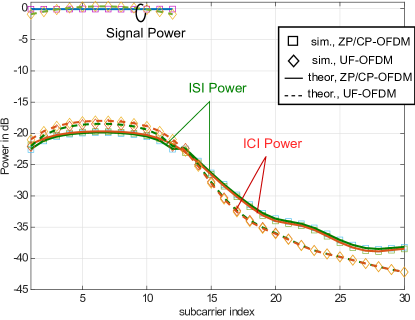
(a) VehB-Channel [24] with $f_{\mathrm{D}}T_{s}=3\times 10^{-5}$

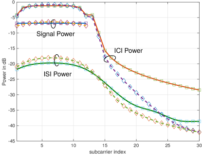
(b) VehB-Channel [24] with $f_{\mathrm{D}}T_{s}=1.5\times 10^{-3}$

Fig. 1: Signal, ICI and ISI power analysis; simulation versus theoretical analysis

In Fig. 1a, the power distributions of the signal, ICI and ISI component are plotted over subcarriers with UF-OFDM and CP/ZP-OFDM waveforms respectively where a relatively small Doppler spread of $f_{\mathrm{D}}T_{s}=3\times 10^{-5}$ is considered. The results obtained by simulations and the derived analytical approach match very well. The signal power variation is due to the FIR-filtering in UF-OFDM. For comparably large Doppler spread of $f_{\mathrm{D}}T_{s}=1.5\times 10^{-3}$, Fig. 1b shows the signal, ICI and ISI power level respectively. In contrast to UF-OFDM, the signal power of CP/ZP-OFDM remains constant over subcarriers. The large signal power degradation is mainly due to the large Doppler spread. While the ICI level increases because of Doppler spread, the ISI power hardly changes with Doppler spreads (It means that the average ISI power over the entire bandwidth is independent of the Doppler spread while its distribution over subcarriers slightly changes). We note that the Monte-Carlo simulation approach is quite computational intensive because of the correlation between the channel coefficients at arbitrary two time instants in comparison to the analytical approach relying solely on the correlation statistics in time and frequency domain. It is also noteworthy to mention that CP/ZP-OFDM is capable of mitigating delay spread induced ISI and ICI while UF-OFDM generates less out-of-band emission to adjacent channels/subcarriers.

IV-B Downlink SINR

In the downlink, $M=85$ subbands are occupied for data transmission (to multiple and/or single user) which corresponds to $1020$ subcarriers. The downlink signal arrives at one user through a wireless channel with certain delay spread and Doppler spread. The average SINR over all the subcarriers are shown in the following. Fig. 2 shows the SINR performance

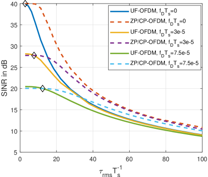
Fig. 2: SINR versus delay spread

of CP/ZP-OFDM and UF-OFDM over a variety of rms channel delay spread. Due to the absence of CP/ZP in UF-OFDM, it is vulnerable to delay spread whereas CP/ZP-OFDM achieves much high SINR thanks to CP/ZP. With increasing Doppler spread, the SINR decreases because of ICI. It can be observed that UF-OFDM slightly outperforms CP/ZP-OFDM at the low delay spread region since the filtering in UF-OFDM improves its spectral compactness leading to less inter-subband interference compared to CP/ZP-OFDM. The intersection of two curves with the same Doppler spread parameter, i.e., that of UF- and CP/ZP-OFDM respectively, are marked by diamond in the figure. The SINR gain is not significant due to two reasons; the FIR-filter is not optimized; the intra-subband interference caused by Doppler spread is much larger.

Next, we show the SINR performance of both system over Doppler spreads in Fig. 3. The inserted CP/ZP is extremely effective for mitigating delay spread -induced ISI and ICI. It has no impact on the Doppler-induced ICI. From the results, it can be concluded that both waveform techniques have similar performance. To be more precisely, UF-OFDM shall be favored with low delay spread high Doppler spread channels and CP/ZP-OFDM is superior with large delay spread and low Doppler spread channels.

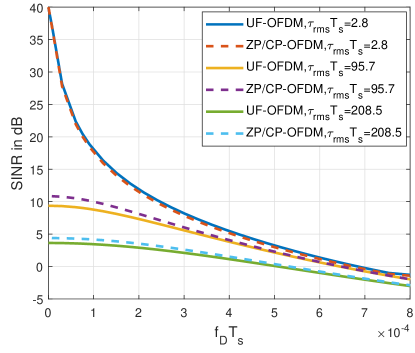
Fig. 3: SINR versus Doppler spread

Finally, we show in Fig. 4 and in Fig. 6 the SINR heat-map for different channels with time and frequency selectivity parameters with CP/ZP-OFDM and UF-OFDM waveforms, respectively.

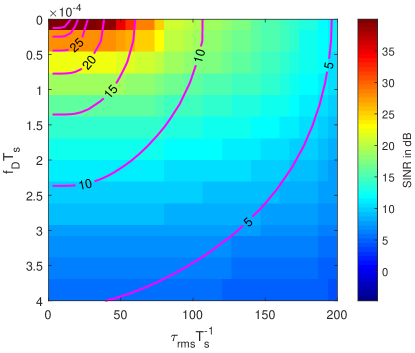
Fig. 4: SINR of CP-OFDM

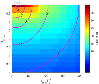
Fig. 5: SINR of ZP-OFDM

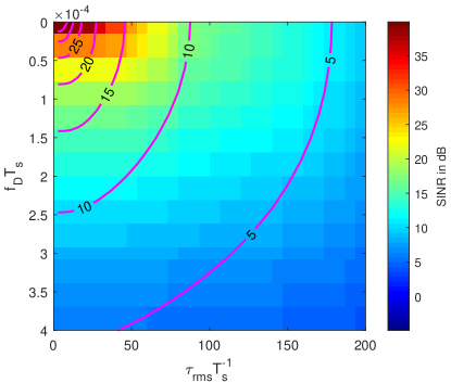
Fig. 6: SINR of UF-OFDM

The contour lines are also depicted in both figures. It is obvious that CP/ZP-OFDM provides better delay spread protection than UF-OFDM. It may not be so obvious from the figures that UF-OFDM provides small to marginal gain over CP/ZP-OFDM with increasing Doppler-spreads. It seems that in the downlink transmission, CP/ZP-OFDM outperforms UF-OFDM in terms of delay spread while it achieves only slightly worse performance at same channel Doppler-spread. However, we remark that cyclic prefix or zero pre-/postfix can also be easily inserted in UF-OFDM for delay spread protection with further loss of spectral efficiency.

IV-C Uplink SINR

In the uplink, the signals of different users arrive at the basestation through very different channels. The SINR is thus very different, depending not exclusively on its own channel conditions but also on the adjacent channel conditions. We consider three user equipments (UEs) each with the bandwidth of $6$ subbands. The per-subcarrier SINR is shown in Fig. 7 along with the channel conditions of each UE.

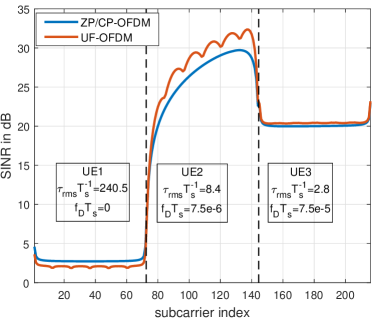
Fig. 7: SINR over frequencies in a heterogeneous uplink multiuser scenario

The UE1 is stationary but with relatively long channel delay; the UE2moves at relatively slow speed (corresponding to $50\,\mathrm{kmh}$ with the carrier frequency of $2.5\,\mathrm{GHz}$ and total bandwidth of $15\,\mathrm{MHz}$) and the channel delay spread is also comparatively small; the UE3 moves at very high speed and it experiences nearly flat fading. UE1 achieves $0.7\,\mathrm{dB}$ SINR gain with CP/ZP-OFDM while it generates larger interference to the adjacent UE2. UE3 achieves $0.3\,\mathrm{dB}$ SINR gain with UF-OFDM and generates less interference to UE2 simultaneously for the high Doppler low delay channel case. In this heterogeneous traffic setting, the UE2 can achieve the SINR gain of $2.1\,\mathrm{dB}$ with UF-OFDM.

	CP/ZP-OFDM	UF-OFDM
UE1	1.55 bpcu	1.40 bpcu
UE2	9.04 bpcu	9.74 bpcu
UE3	6.73 bpcu	6.85 bpcu
sum	17.32 bpcu	17.99 bpcu

Table I: Channel Capacity

In Tab. I, the (lower bound) of the channel capacity per UE and the sum capacity is compared. The UE1 looses $0.15\,\mathrm{bpcu}$ (bit per channel use) applying filtering instead of CP/ZP, however, by doing this it is capable of boosting the adjacent users’ channel capacity by $0.7\,\mathrm{bpcu}$ leading to the overall sum capacity gain of $0.67\,\mathrm{bpcu}$.

IV-D Discussion

The results reveal that CP/ZP-OFDM is profoundly resilient to delay spread and vulnerable to Doppler spread while UF-OFDM on the opposite offers better Doppler-spread protection, both relying on the same amount of redundancy in the form of filtering and CP/ZP. In the case of downlink transmission where the channel remains homogeneous within entire bandwidth, CP/ZP-OFDM can operate on a wider range of channel characteristics while UF-OFDM (yet with non optimized filtering procedure) offers slightly SINR gain in low delay spread region. However, if channel characteristics of adjacent channels are extremely diverse as in the uplink, UF-OFDM might be better to support a larger variety of users with different speed profiles. Furthermore, we note that the FIR-filter is somewhat arbitrarily chosen in UF-OFDM and not optimized for the channel statistics. An optimal design of FIR-filtering (including zero-padding or cyclic prefix) could be an interesting extension of this work.

V Conclusion

The impact of delay spread and Doppler spread of general wireless channels is analytically addressed in the context of orthogonal multicarrier waveforms, particularly CP/ZP-OFDM and UF-OFDM. The derived analytical formula is in closed-form assuming known Doppler-spectrum, power delay profile (PDP) and simple one-tap equalizer. The results can be applied to any channel and ZP-/CP-/UF-OFDM transceiver parameters in terms of delay, Doppler spread, ZP/CP/filter length and receive windows. With the obtained analytical formula, the SINR analysis and comparison between the waveforms is facilitated without requiring computationally extensive simulations. The SINR comparison shows that CP/ZP-OFDM can efficiently mitigate the ISI/ICI caused by channel delay spread and is vulnerable to Doppler spread while UF-OFDM just exhibits the opposite property. Future works involve the FIR-filter optimization and the window design for both waveforms. More sophisticated and low complexity equalizer design and optimal combination of FIR-filtering and CP/ZP-insertion could be tackled.

Appendix A ISI in CP/ZP-OFDM

Inserting (13) and (1) into (14), we obtain

$$\mathbf{Y}_{\mathrm{ISI,O}}=\mathbf{F}_{N}\mathbf{C}_{\mathrm{R}}\tilde{\mathbf{w}}_{\mathrm{I}}\tilde{\mathbf{h}}_{m-1}\tilde{\mathbf{C}}_{\mathrm{A}}\mathbf{F}^{H}\cdot\mathbf{X}_{m-1}$$

where $\tilde{\mathbf{C}}_{\mathrm{A}}$ is padded with zero rows to align the matrix dimension to $2N\times N$. Next, we incorporate the frequency and Doppler description of the time-varying channel matrix into the equation, which reads

$$\mathbf{Y}_{\mathrm{ISI},\mathrm{O}}=\underset{\mathbf{W}_{\mathrm{I}}}{\underbrace{\mathbf{F}_{N}\mathbf{C}_{\mathrm{R}}\tilde{\mathbf{w}}_{\mathrm{I}}\mathbf{F}_{2N}^{H}}}\underset{\mathbf{H}_{m-1}}{\underbrace{\mathbf{F}_{2N}\tilde{\mathbf{h}}_{m-1}\mathbf{F}_{2N}^{H}}}\underset{\mathbf{T}_{\mathrm{O}}}{\underbrace{\mathbf{F}_{2N}\tilde{\mathbf{C}}_{\mathrm{A}}\mathbf{F}^{H}}}\cdot\mathbf{X}_{m-1}.$$

If the CP/ZP length exceeds maximum delay spread, i.e., $D\leq L$, then $\mathbf{C}_{\mathrm{R}}\tilde{\mathbf{w}}_{\mathrm{I}}=\mathbf{0=W}_{\mathrm{I}}$, hence no ISI is present. More generally, $\mathbf{W}_{\mathrm{I}}$ is highly structured like circulant matrices. Let $\mathbf{\boldsymbol{\mathbf{\omega}}}_{i}$ be the $i$th row vector of $\mathbf{W}_{\mathrm{I}}$, it can be obtained by cyclically shifting the first row by $2i$ elements and multiplying a phase shift, i.e., $\boldsymbol{\omega}_{i}=\mathrm{circshift}\left[\boldsymbol{\omega}_{0}\cdot e^{j4\pi iL/N},2i\right].$ Its first row vector is simply the 2N-IFFT of the ISI window, i.e., $\boldsymbol{\omega}_{0}^{T}=\frac{1}{\sqrt{N}}\mathbf{F}_{2N}^{H}\cdot\left[\mathbf{0}_{N+2L,}\>v_{L+1},\cdots,v_{D},\mathbf{0}_{N-L-D}\right]^{T}.$ $\mathbf{H}_{m-1}$ is one realization of the 2 dimensional Fourier transform of the doubly selective channel of the $m-1$th symbol. $\mathbf{T}_{\mathrm{O}}$ models the pulse shaping operation at transmitter (or CP/ZP insertion in OFDM), which has the similar structure as $\mathbf{W}_{\mathrm{I}}$, i.e., $\boldsymbol{t}_{i}=\mathrm{circshift}\left[\boldsymbol{t}_{0}\cdot e^{-j2\pi iL/N},2i\right].$ Its $i$th column $\mathbf{t}_{i}$ is cyclically shifted of $\mathbf{t}_{1}$ by $2i$ and $\mathbf{t}_{0}=\frac{1}{\sqrt{N}}\mathbf{F}_{2N}\cdot\left[\mathbf{1}_{N+L},\mathbf{0}_{N-L}\right]^{T}$.

Appendix B ISI in UF-OFDM

Inserting (2) into (19), we obtain

$$\mathbf{Y}_{\mathrm{ISI,U}}=\underset{\mathbf{W}_{\mathrm{I,U}}}{\underbrace{\tilde{\mathbf{F}}_{2N}\tilde{\mathbf{w}}_{\mathrm{I}}\mathbf{F}_{2N}^{H}}}\underset{\mathbf{H}_{m-1}}{\underbrace{\mathbf{F}_{2N}\tilde{\mathbf{h}}_{m-1}\mathbf{F}_{2N}^{H}}}\underset{\mathbf{T}_{\mathrm{U}}}{\underbrace{\mathbf{F}_{2N}\tilde{\mathbf{G}}\mathbf{F}^{H}}}\cdot\mathbf{X}_{m-1},$$

where $\mathbf{W}_{\mathrm{I,U}}$ has the same “circulant” property as in CP/ZP-OFDM. However, its first row is given by $\boldsymbol{\omega}_{0,\mathrm{U}}^{T}=\frac{1}{\sqrt{N}}\mathbf{F}_{2N}^{H}\cdot\left[\mathbf{0}_{N+L,}\>v_{1},\cdots,v_{D},\mathbf{0}_{N-L-D}\right]^{T}$ and the per row constant phase shift equals $e^{j2\pi iL/N}$. This leads to nonzero ISI whenever $D\geq 0$ due to the absence of guard interval in time. Because of FIR-filtering, the filter response is incorporated in the pulse-shaping matrix, it can be show that $\mathbf{T}_{\mathrm{U}}=\mathrm{diag}\left(\mathbf{F}_{2N}[g_{i,0},\cdots,g_{i,L_{\mathrm{F}}},\mathbf{0}_{2N-L_{F}-1}]\right)\cdot\tilde{\mathbf{T}}_{\mathrm{U}}$ and $\tilde{\mathbf{T}}_{\mathrm{U}}$ has the same “circulant” property as $\mathbf{T}_{\mathrm{O}}$. The first column of $\tilde{\mathbf{T}}_{\mathrm{U}}$ is given by $\tilde{\mathbf{t}}_{1}=\sqrt{2}\mathbf{F}_{2N}\cdot\left[\mathbf{1}_{N},\mathbf{0}_{N}\right]^{T}$.

Appendix C ISI power

We derive the average ISI power per subcarrier for both UF- and CP/ZP-OFDM, since the two systems differ only in pulse shaping and receive processing. Consider the ISI part,

$$\mathbf{Y}_{\mathrm{ISI}}=\mathbf{W}_{\mathrm{I}}\mathbf{H}_{m-1}\mathbf{T}\mathbf{s}_{m-1}$$ (20)

where $\mathbf{T}$ denotes the pulse-shaping matrix for either UF- or CP/ZP-OFDM signals. Thus, the power of ISI at $k$th subcarrier can be obtained by

$$\mathrm{P}_{\mathrm{ISI}}\left(k\right) =\mathrm{E\left[Y_{ISI,\mathit{k}}\cdot Y_{ISI,\mathit{k}}^{H}\right]}$$

$$=\mathbf{W}_{\mathrm{I},k}\mathrm{E\left[\mathbf{H}_{m-1}\mathbf{T}\underset{\mathbf{I}}{\underbrace{\mathbf{s}_{m-1}\mathbf{s}_{m-1}^{\mathit{H}}}}\mathbf{T}^{\mathit{H}}\mathbf{H}_{m-1}^{\mathit{H}}\right]\mathbf{W}_{\mathrm{I},\mathit{k}}^{\mathit{H}}}$$

$$=\mathbf{W}_{\mathrm{I},k}\mathrm{\underset{\mathbf{R}_{H}}{\underbrace{\mathrm{E}\left[\mathbf{H}_{m-1}\mathbf{T}\mathbf{T}^{H}\mathbf{H}_{m-1}^{H}\right]}}\mathbf{W}_{\mathrm{I},\mathit{k}}^{\mathit{H}}}$$

where $\mathbf{W}_{\mathrm{I},k}$ denotes the $k$th row of the receive matrix $\mathbf{W}_{\mathrm{I}}$.

The frequency-Doppler representation of the time-varying multipath channel is defined as $\mathbf{H}_{m}=\mathbf{F}_{2N}\tilde{\mathbf{h}}_{m}\mathbf{F}_{2N}^{H}$. It is straightforward to show that $\left[\mathbf{H}_{m}\right]_{kn}={\displaystyle\sum_{l}}{\displaystyle\sum_{p}}\left[\tilde{\mathbf{h}}_{m}\right]_{pl}e^{j\pi\frac{nl-kp}{N}}$. Thus, the correlation between two arbitrary elements is given by

$$r_{kk^{\prime}nn^{\prime}}= {\displaystyle\sum_{l,l^{\prime},p,p^{\prime}}}\left[\tilde{\mathbf{h}}_{m}\right]_{pl}\left[\tilde{\mathbf{h}}_{m}\right]_{p^{\prime}l^{\prime}}^{*}e^{j\pi\frac{nl-kp-n^{\prime}l^{\prime}+k^{\prime}p^{\prime}}{N}}$$

$$= {\displaystyle\sum_{l,p,\Delta p=\Delta l}}\rho_{p-l}R_{t}\left(\Delta l\right)e^{j\pi\frac{l\left(n-n^{\prime}\right)-p\left(k-k^{\prime}\right)-\left(n^{\prime}-k^{\prime}\right)\Delta l}{N}}$$

$$= \underset{R_{f}\left(k-k^{\prime}\right)}{\underbrace{\left[{\displaystyle\sum_{p}\rho_{p}}e^{j\pi\frac{-p\left(k-k^{\prime}\right)}{N}}\right]}}$$

$$\cdot\underset{\left[\mathbf{R}_{D}^{*}\right]_{\left(n^{\prime}-k^{\prime}\right)\left(n-k\right)}}{\underbrace{\left[{\displaystyle\sum_{l,\Delta l}}R_{t}\left(\Delta l\right)e^{j\pi\frac{l\left(n-n^{\prime}-k-k^{\prime}\right)-\left(n^{\prime}-k^{\prime}\right)\Delta l}{N}}\right]}}$$

where $R_{f}\left(\cdot\right)$ is the frequency correlation function and $\mathbf{R}_{D}$ is the Doppler covariance matrix (see Appendix D). As the consequence of WSSUS, the total correlation in Doppler-frequency domain is given by the product of frequency and Doppler correlation.

The computation of $\mathbf{R}_{\mathrm{H}}$ is as follows. The element $r_{ij}$ of the matrix can be obtained by

$$r_{ij} =\mathrm{E\left[\mathbf{H}_{\mathit{m\mathrm{-1},i}}\mathbf{T}\mathbf{T}^{\mathit{H}}\mathbf{H}_{\mathit{m\mathit{\mathrm{-1}},j}}^{\mathit{H}}\right]}$$

$$=\mathrm{tr}\left[\mathbf{T}\mathbf{T}^{H}\mathrm{E}\left(\mathbf{H}_{\mathit{m\mathrm{-1},j}}^{\mathit{H}}\mathbf{H}_{\mathit{m\mathrm{-1},i}}\right)\right]$$

$$\mathrm{=tr\left[\mathbf{\boldsymbol{\varGamma}}_{T}\left(R_{f}\left(i-j\right)\mathbf{P}_{j}\mathbf{R}_{D}^{*}\mathbf{P}_{i}\right)\right]}$$

$$=R_{f}\left(i-j\right)\mathrm{tr}\left[\mathbf{\boldsymbol{\varGamma}}_{T}\mathbf{P}_{j}\mathbf{R}_{\mathrm{D}}^{*}\mathbf{P}_{i}\right]$$

where $\mathbf{P}_{j}$ and $\mathbf{P}_{i}$ are permutation matrices (moves $j$ elements down and $i$ elements to the right), $\mathbf{\boldsymbol{\varGamma}}_{T}=\mathbf{T}\mathbf{T}^{H}$, $\mathbf{R}_{f}$ is the frequency correlation matrix determined by the channel PDP and $\mathbf{R}_{\mathrm{D}}$ is the Doppler correlation function determined by the time selectivity (The computation of both correlation matrices is provided in Appendix D with the WSSUS assumption). Faster computation is thus row-wise (or column-wise)

$$\mathbf{r}_{j}=\mathrm{gtr\left[\mathbf{\boldsymbol{\varGamma}}_{T}\mathbf{P}_{j}\mathbf{R}_{D}^{*}\right]\circ\mathbf{R}_{f,\mathit{j}}}$$ (21)

where $\circ$ denotes Hadamard product of two matrices, $\mathbf{r=}\mathrm{gtr}\left[\mathbf{A}\right]$ operator of square $N\times N$ matrix $\mathbf{A}$ is defined as $r_{j}={\displaystyle\sum_{i=0}^{N-1}}a_{\left\langle i+j\right\rangle_{N},i}$. Hence, the power of ISI can also be analytically calculated.

Appendix D Doppler and frequency correlation matrices

The frequency correlation matrix $\mathbf{R}_{f}$ is generally circulant, the element is given by $\left[\mathbf{R}_{f}\right]_{ij}=R_{f}\left(i-j\right)$, see 6 for EDPDP channel. It is therefore sufficient to calculate the first row of $\mathbf{R}_{f}$ which is the Fourier transform of the channel PDP.

For the often ignored Doppler-domain correlation, it suffices to consider an arbitrary $i$th tap $h_{im}$. Denote the $k$th and $p$th Doppler response by $H_{D}\left(k\right)=\frac{1}{\sqrt{N}}{\displaystyle\sum_{m=0}^{N-1}}h_{im}e^{j\frac{2\pi}{N}mk}$ and $H_{D}\left(p\right)$, respectively. The correlation is therefore given by

$$\left[\mathbf{R}_{D}\right]_{kp} =\frac{1}{N}\mathrm{E}\left\{{\displaystyle\sum_{n}{\displaystyle\sum_{m}}}h_{im}h_{in}^{*}e^{j\frac{2\pi}{N}\left(mk-pn\right)}\right\}$$

$$=\frac{1}{N}\rho_{i}{\displaystyle\sum_{n}{\displaystyle\sum_{m}}}R_{t}\left(m-n\right)e^{j\frac{2\pi}{N}\left(mk-pn\right)}.$$

Hence the correlation matrix is 2D Fourier transform of the Toeplitz matrix with elements $\left[\mathbf{R}_{t}\right]_{nm}=R_{t}\left(m-n\right)$, i.e., $\mathbf{R}_{D}=\mathbf{F}\mathbf{R}_{t}\mathbf{F}^{H}$.

Appendix E ICI and signal

Similar to the analysis of ISI, we can write

$$\mathbf{Y}_{\mathrm{s}}+\mathbf{Y}_{\mathrm{ICI}}=\mathbf{W}_{D}\mathbf{H}_{m}\mathbf{T}\mathbf{s}_{m}.$$

The signal term and ICI term shall be easily separated. Consider an arbitrary subcarrier $k$, we can obtain

$$Y_{\mathrm{s},\mathit{k}} =\mathbf{W}_{\mathrm{D},k}\mathbf{H}_{m}\mathbf{T}_{s,k}s_{m,k}$$

$$Y_{\mathrm{ICI},\mathit{k}} =\mathbf{W}_{\mathrm{D},k}\mathbf{H}_{m}\bar{\mathbf{T}}_{k}\bar{\mathbf{s}}_{m,k}$$

where $\bar{\mathbf{T}}_{s,k}$ and $\bar{\mathbf{s}}_{m,k}$ denote the residual matrix and vector after deleting the $k$th column or element, respectively. Thus the signal power and ICI power can be computed according to

$$\mathrm{P}_{\mathrm{S}}\left(k\right) =\mathrm{E\left[Y_{s,\mathit{k}}\cdot Y_{s,\mathit{k}}^{H}\right]}$$

$$=\mathbf{W}_{\mathrm{D},k}\mathrm{\underset{\mathbf{R}_{H,S}}{\underbrace{\mathrm{E}\left[\mathbf{H}_{m}\mathbf{T}_{s,\mathit{k}}\mathbf{T}_{s,\mathit{k}}^{H}\mathbf{H}_{m}^{H}\right]}}\mathbf{W}_{\mathrm{D},\mathit{k}}^{\mathit{H}}}$$

$$\mathrm{P}_{\mathrm{ICI}}\left(k\right) =\mathrm{E\left[Y_{ICI,\mathit{k}}\cdot Y_{ICI,\mathit{k}}^{H}\right]}$$

$$=\mathbf{W}_{\mathrm{D},k}\mathrm{\underset{\mathbf{R}_{H,ICI}}{\underbrace{\mathrm{E}\left[\mathbf{H}_{m}\bar{\mathbf{T}}_{\mathit{k}}\mathbf{\bar{T}}_{\mathit{k}}^{H}\mathbf{H}_{m}^{H}\right]}}\mathbf{W}_{\mathrm{D},\mathit{k}}^{\mathit{H}}}.$$

References

- [1] B. Muquet, Z. Wang, G. B. Giannakis, M. de Courville, and P. Duhamel, “Cyclic prefixing or zero padding for wireless multicarrier transmissions?” IEEE Transactions on Communications, vol. 50, no. 12, pp. 2136–2148, Dec 2002.
- [2] V. Vakilian, T. Wild, F. Schaich, S. ten Brink, and J. F. Frigon, “Universal-filtered multi-carrier technique for wireless systems beyond LTE,” in IEEE Globecom, Dec 2013, pp. 223–228.
- [3] T. Wild, F. Schaich, and Y. Chen, “5G air interface design based on Universal Filtered (UF-)OFDM,” in 19th International Conference on Digital Signal Processing (DSP), Aug 2014, pp. 699–704.
- [4] F. Schaich and T. Wild, “Relaxed synchronization support of universal filtered multi-carrier including autonomous timing advance,” in 2014 11th International Symposium on Wireless Communications Systems (ISWCS), Aug 2014, pp. 203–208.
- [5] S. Wang, J. S. Thompson, and P. M. Grant, “Closed-Form Expressions for ICI/ISI in Filtered OFDM Systems for Asynchronous 5G Uplink,” IEEE Transactions on Communications, vol. 65, no. 11, pp. 4886–4898, Nov 2017.
- [6] L. Zhang, A. Ijaz, P. Xiao, A. Quddus, and R. Tafazolli, “Subband filtered multi-carrier systems for multi-service wireless communications,” IEEE Transactions on Wireless Communications, vol. 16, no. 3, pp. 1893–1907, March 2017.
- [7] M. Wu, J. Dang, Z. Zhang, and L. Wu, “An advanced receiver for universal filtered multicarrier,” IEEE Transactions on Vehicular Technology, vol. 67, no. 8, pp. 7779–7783, Aug 2018.
- [8] B. Farhang-Boroujeny and H. Moradi, “OFDM inspired waveforms for 5G,” IEEE Communications Surveys Tutorials, vol. 18, no. 4, pp. 2474–2492, Fourthquarter 2016.
- [9] L. Zhang, P. Xiao, and A. Quddus, “Cyclic prefix-based universal filtered multicarrier system and performance analysis,” IEEE Signal Processing Letters, vol. 23, no. 9, pp. 1197–1201, Sep. 2016.
- [10] Z. Zhang, H. Wang, G. Yu, Y. Zhang, and X. Wang, “Universal filtered multi-carrier transmission with adaptive active interference cancellation,” IEEE Transactions on Communications, vol. 65, no. 6, pp. 2554–2567, June 2017.
- [11] Y. Liu, X. Chen, Z. Zhong, B. Ai, D. Miao, Z. Zhao, J. Sun, Y. Teng, and H. Guan, “Waveform design for 5G networks: Analysis and comparison,” IEEE Access, vol. 5, pp. 19 282–19 292, 2017.
- [12] X. Chen, L. Wu, Z. Zhang, J. Dang, and J. Wang, “Adaptive modulation and filter configuration in universal filtered multi-carrier systems,” IEEE Transactions on Wireless Communications, vol. 17, no. 3, pp. 1869–1881, March 2018.
- [13] D. Han, J. Moon, D. Kim, S. Chung, and Y. H. Lee, “Combined subband-subcarrier spectral shaping in multi-carrier modulation under the excess frame length constraint,” IEEE Journal on Selected Areas in Communications, vol. 35, no. 6, pp. 1339–1352, June 2017.
- [14] D. Han, J. Moon, J. Sohn, S. Jo, and J. H. Kim, “Combined window-filter waveform design with transmitter-side channel state information,” IEEE Transactions on Vehicular Technology, vol. 67, no. 9, pp. 8959–8963, Sep. 2018.
- [15] X. Wang, T. Wild, and F. Schaich, “Filter Optimization for Carrier-Frequency- and Timing-Offset in Universal Filtered Multi-Carrier Systems,” in IEEE 81st Vehicular Technology Conference (VTC Spring), May 2015, pp. 1–6.
- [16] M.-F. Tang and B. Su, “Filter optimization of low out-of-subband emission for universal-filtered multicarrier systems,” in 2016 IEEE International Conference on Communications Workshops (ICC), May 2016, pp. 468–473.
- [17] J. Wen, J. Hua, W. Lu, Y. Zhang, and D. Wang, “Design of waveform shaping filter in the UFMC system,” IEEE Access, vol. 6, pp. 32 300–32 309, 2018.
- [18] Y. Li and L. J. Cimini, “Bounds on the interchannel interference of OFDM in time-varying impairments,” IEEE Transactions on Communications, vol. 49, no. 3, pp. 401–404, Mar 2001.
- [19] P. Robertson and S. Kaiser, “The effects of Doppler spreads in OFDM(A) mobile radio systems,” in Gateway to 21st Century Communications Village. VTC 1999-Fall. IEEE VTS 50th Vehicular Technology Conference (Cat. No.99CH36324), vol. 1, 1999, pp. 329–333 vol.1.
- [20] P. Schniter, “Low-complexity equalization of OFDM in doubly selective channels,” IEEE Transactions on Signal Processing, vol. 52, no. 4, pp. 1002–1011, April 2004.
- [21] S. Das and P. Schniter, “Max-SINR ISI/ICI-Shaping Multicarrier Communication Over the Doubly Dispersive Channel,” IEEE Transactions on Signal Processing, vol. 55, no. 12, pp. 5782–5795, Dec 2007.
- [22] L. Rugini, P. Banelli, and G. Leus, “OFDM Communications over Time-Varying Channels,” in Wireless Communications Over Rapidly Time-Varying Channels, F. Hlawatsch and G. Matz, Eds. The Boulevard, Langford Lane, Kidlington, Oxford OX5 1GB, UK: Elsevier, 2011, ch. 7, pp. 285–336.
- [23] T. Wang, J. G. Proakis, E. Masry, and J. R. Zeidler, “Performance degradation of OFDM systems due to Doppler spreading,” IEEE Transactions on Wireless Communications, vol. 5, no. 6, pp. 1422–1432, June 2006.
- [24] Recommendation ITU-R M.1225, “Guidlines for evaluation of radio transmission technologies for IMT-2000,” ITU, Tech. Rep., 1997.