An NMPC Approach using Convex Inner Approximations for
Online Motion Planning with Guaranteed Collision Avoidance

Abstract

Even though mobile robots have been around for decades, trajectory optimization and continuous time collision avoidance remain subject of active research. Existing methods trade off between path quality, computational complexity, and kinodynamic feasibility. This work approaches the problem using a nonlinear model predictive control (NMPC) framework, that is based on a novel convex inner approximation of the collision avoidance constraint. The proposed Convex Inner ApprOximation (CIAO) method finds kinodynamically feasible and continuous time collision free trajectories, in few iterations, typically one. For a feasible initialization, the approach is guaranteed to find a feasible solution, i.e. it preserves feasibility. Our experimental evaluation shows that CIAO outperforms state of the art baselines in terms of planning efficiency and path quality. Experiments on a robot with 12 states show that it also scales to high-dimensional systems. Furthermore real-world experiments demonstrate its capability of unifying trajectory optimization and tracking for safe motion planning in dynamic environments.

I INTRODUCTION

Several existing mobile robotics applications (e.g. intra-logistic and service robotics) require robots to operate in dynamic environments among other agents, such as humans or other autonomous systems. In these scenarios, the reactive avoidance of unforeseen dynamic obstacles is an important requirement. Combined with the objective of reaching optimal robot behavior, this poses a major challenge for motion planning and control and remains subject of active research.

Recently several researchers have tackled the obstacle avoidance problem by formulating and solving optimization problems [1, 2, 3, 4, 5, 6, 7, 8, 9, 10, 11, 12, 13, 14]. This approach is well suited for finding locally optimal solutions, but generally gives no guarantee of finding the global optimum. Most methods therefore rely on the initialization by an asymptotically optimal sampling-based planner [15, 16, 17]. A shortcoming of most common trajectory optimization methods is that they are incapable of respecting kinodynamic constraints, e.g. bounds on the acceleration, and typically lack a notion of time in their predictions, [1, 2, 3, 4]. These approaches are typically limited to the optimization of paths rather than trajectories and impose constraints by introducing penalties.

The increase of computing power and the availability of fast numerical solvers, as discussed in [18], has given rise to model predictive control (MPC) based approaches, e.g. [3, 4, 6, 5, 7]. In this framework, an optimal control problem (OCP) is solved in every iteration. These methods succeed in finding kinodynamically [6, 7, 5] or kinematically [3, 4, 5] feasible trajectories, but typically use penalty terms in the cost function that offer no safety guarantees [7] or require that obstacles are given as a set of convex hulls [4].

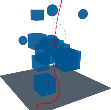
Figure 1: CIAO trajectories for the Astrobee robot (top row) in red and for a unicycle robot (last two rows) with three different maximum speeds $v_{\max}$ and corresponding minimum distances $\underline{d}$ (see (5)): green - slow, red - normal, blue - fast. The boxes and spheres represent obstacles, the turquoise dots the reference path. A wider spacing between the dots indicates a higher speed. The start is always located in the bottom and the goal in the top. It is clearly visible that CIAO maintains higher distances to obstacles for higher speeds.

Contribution

This work presents CIAO, a nonlinear (NMPC) based approach to real-time collision avoidance for single body robots. It preserves feasibility across iterations and uses a novel, convex formulation of the collision avoidance constraint that is compatible with many implementations of the distance function, even discrete ones like distance fields. To the best of authors’ knowledge, CIAO is the first real-time capable NMPC approach that guarantees continuous time collision free trajectories and is agnostic of the distance function’s implementation. The method’s efficacy is demonstrated and evaluated in simulation and real-world using robots with nonlinear, constrained dynamics and state of the art baselines.

Structure

The paper is structured as follows: The related work is discussed in Section II and Section III introduces the problem we want to solve. Section IV details CIAO alongside some considerations on feasibility, safety and practical challenges. In Section V we detail how CIAO can be used for trajectory optimization and receding horizon control (RHC). The experiments and results are discussed in Section VI. A summary and an outlook is given in Section VII.

II Related Work

Trajectory optimization methods try to find time-optimal and collision-free robot trajectories by formulating and solving an optimization problem [1, 2, 8, 3, 4, 5, 6, 10, 7, 9, 11, 12, 13, 14]. Classical approaches to obstacle avoidance include [19, 20, 21, 22, 23]. These approaches do neither produce optimal trajectories, nor unify planning and control, nor account for complex robot dynamics.

A simple and effective method that is still used in practice, is the elastic-band algorithm [1]. The computed paths, however, are generally non-smooth, i.e. they are not guaranteed to satisfy kinodynamic constraints, nor does this algorithm compute a velocity profile. Like Zhu et al. [9], our approach aims to fix this shortcoming, while building up on the notion of (circular) free regions. Instead of optimizing velocity profile and path length separately, as done in [9, 1], we optimize them jointly utilizing an nonlinear (NMPC) setup. Also Rösmann et al. [10] provide an approach which combines elastic-band with an optimization algorithm. Contrarily to ours, their approach does not enforce obstacle avoidance as constraint, and requires a further controller for trajectory tracking.

Nowadays optimization based methods receive increasingly more attention. Popular methods include CHOMP [3], TrajOpt [4], OBCA [6], and GuSTO [7], which have been shown to produce smooth trajectories efficiently. They typically use a simplified system model to compute a path from the current to the goal state (or set), and further need an additional controller to steer the system along the precomputed path. The proposed method, CIAO, is MPC-based and provides algorithms for both trajectory optimization and RHC, simultaneously controlling the robot and optimizing its trajectory.

Also Neunert et al. [14] propose RHC to unify trajectory optimization and tracking, but their approach does not include a strategy for obstacle avoidance. They propose to solve an unconstrained nonlinear program (NLP) online, CIAO on the other hand is solving a constrained NLP online that enforces collision avoidance as constraint.

Frasch et al. [11] propose an MPC with box-constraints to model obstacles and road boundaries. Liniger et al. [12] handle obstacles in a similar way, but apply contouring control, i.e. the approach steers a race car in a corridor around a predefined path. These frameworks do not consider arbitrarily placed obstacles, particularly no moving obstacles, which makes them unsuitable for many applications. In our approach we handle more complex obstacle definitions, modeled according to a generic nonlinear and nonconvex distance function. To this end, we propose a novel constraint formulation that is shown to be a convex inner approximation of the actual collision avoidance constraint.

Herbert et al. [5] propose a hybrid approach to safely avoid dynamic obstacles. The trajectory tracker does not consider the obstacles explicitly, but relies on the planning layer. The method proposed in this work presents a unified approach for all robot motion planing, control, and obstacle avoidance, using constrained NMPC.

The recently proposed method GuSTO [7] uses sequential convex programming (SCP), like other common algorithms, e.g. [4, 12, 11, 10]. SCP requires a full convexification of the originally nonlinear and nonconvex trajectory optimization problem. This is accomplished by linearizing the system model and incorporating paths constraints, including collision avoidance, as penalties in the objective function. In general these approximations may lead to infeasible, i.e. colliding or kinodynamically intractable trajectories. Typically several SCP iterations are required to find a feasible solution. CIAO, on the other hand, solves partially convexified NLPs, using a convex inner approximation of the collision avoidance constraint, and finds feasible solutions in less iterations, typically one. The individual iterations are computationally cheaper and feasibility is preserved. Since the dynamical model is accounted for by the NLP-solver, linearization errors are minimized.

Finally CIAO can be considered as a trust region method [24], where the nonlinear state constraints are approximated with a convex inner approximation.

III PROBLEM FORMULATION

We want to find a kinodynamically feasible, collision free trajectory by formulating and solving a constrained OCP. Kinodynamic feasibility is ensured by using a dynamical model to simulate the robot’s behavior and collision avoidance is achieved constraining the robot to positions with a minimum distance $\underline{d}$ to all obstacles.

The occupied set $\mathcal{O}$ is defined as the set of points in the robot’s workspace $\mathcal{W}\subseteq\mathbb{R}^{n}$ that are occupied by obstacles. The Euclidean distance to the closest obstacle for any point $\mathbf{p}\in\mathcal{W}$ is given by the distance function $d_{\mathcal{O}}:\mathcal{W}\to\mathbb{R}$:

$$d_{\mathcal{O}}(\mathbf{p})=d(\mathbf{p};\mathcal{O})=\underset{\mathbf{o}\in\mathcal{O}}{\min}\left\lVert\mathbf{p}-\mathbf{o}\right\rVert_{2}.$$ (1)

For the sake of simplicity we assume that the robot’s shape is contained in an $n$-dimensional sphere with radius $<\underline{d}$ and center point $\mathbf{p}$. Collision avoidance can now be achieved by requesting that the distance function at the robot’s position $\mathbf{p}\in\mathcal{W}$ is at least the minimum distance $\underline{d}$:

$$d_{\mathcal{O}}(\mathbf{p})\geq\underline{d},$$ (2)

which is equivalent to $\|\mathbf{p}-\mathbf{o}\|_{2}\geq\underline{d},\forall\,\mathbf{o}\in\mathcal{O}$.

We assume $\underline{d}>0$ to be fixed from now on, to ensure that points in the occupied set $\mathcal{O}$ do not satisfy (2). A point $\mathbf{p}\in\mathcal{W}$ that satisfies (2) is called ‘free’. Further we define the safety margin as the area for which $0<d_{\mathcal{O}}(\mathbf{p})<\underline{d}$ holds.

We can now formulate an OCP that enforces collision avoidance as path constraint: x (⋅), u (⋅)∫_0^T l( x (t), u (t), r(t))  dt   + l_T( x (T), r(T)) x (0)= ¯ x _0 x (T)∈X_T ˙x (t)= f( x (t), u (t)), t ∈[0, T] h( x (t), u (t))≤0, t ∈[0, T] d_ O ( p (t))≥ d , t ∈[0, T], where $\mathbf{x}(\cdot):\mathbb{R}\rightarrow\mathbb{R}^{{n_{\mathrm{\mathbf{x}}}}}$ denotes the robot’s state, $\mathbf{u}(\cdot):\mathbb{R}\rightarrow\mathbb{R}^{{n_{\mathrm{\mathbf{u}}}}}$ is the vector of controls, $\mathbf{r}(\cdot):\mathbb{R}\to\mathbb{R}^{{n_{\mathrm{\mathbf{x}}}}+{n_{\mathrm{\mathbf{u}}}}}$ provides reference states and controls, $T$ is the length of the horizon in seconds, the function $l(\cdot)$ denotes the cost at time point $t$ and $l_{\mathrm{T}}(\cdot)$ the terminal cost, $\overline{\underline{\mathbf{x}}}_{0}$ is robot’s current state, and $\mathbb{X}_{\mathrm{T}}\subseteq\mathbb{R}^{{n_{\mathrm{\mathbf{x}}}}}$ is the set of admissible terminal states. We use the common shorthand $\dot{\mathbf{x}}$ to denote the derivative with respect to time, i.e. $\dot{\mathbf{x}}=\frac{\partial\,\mathbf{x}}{\partial t}$. The function $f$ models the robot’s dynamics and $h$ implements a set of path constraints, e.g. physical limitations of the system, and $\mathbf{p}(t)=S_{\mathbf{p}}\cdot\mathbf{x}(t)\in\mathcal{W}$ denotes the robot’s position with a selector matrix $S_{\mathbf{p}}$ chosen accordingly.

IV CONVEX INNER APPROXIMATION (CIAO)

In this section we describe how we solve the OCP presented in (III) by adopting a convex inner approximation of the actual collision avoidance constraint presented in Sec. III.

First we discretize (III) using a direct multiple shooting scheme as proposed by [25]. The resulting NLP is a function of $\mathbf{r}$, $\overline{\underline{\mathbf{x}}}_{0}$, and the sampling time $\Delta t$. Using the shorthand $\mathbf{x}_{k}=\mathbf{x}(k\cdot\Delta t),~{}k\in\mathbb{Z}$ for cleaner notation, we discretize (III) as: w J( w , r ) x _0 - ¯ x _0=0 x _N∈X_T x _k+1 - F( x _k, u _k; Δt)=0, k=0,…,N-1 h( x _k, u _k)≤0, k=0,…,N d_ O ( p _k)≥ d ,  k=0,…,N, where $\mathbf{w}=[\mathbf{x}_{0}^{\top},\mathbf{u}_{0}^{\top},\ldots,\mathbf{u}_{N-1}^{\top},\mathbf{x}_{N}^{\top}]^{\top}\in\mathbb{R}^{n_{\mathbf{w}}}$ is a vector of optimization variables that contains the stacked controls and states for all $N$ steps in the horizon, similarly $\mathbf{r}$ contains the reference states and controls, $J(\mathbf{w},\mathbf{r})=\sum_{k=0}^{N-1}l(\mathbf{x}_{k},\mathbf{u}_{k},\mathbf{r}_{k})+l_{\mathrm{T}}(\mathbf{x}_{N},\mathbf{r}_{N})$ is the discretized objective, with stage cost $l$ and terminal cost $l_{\mathrm{T}}$, and $F$ models the discretized robot dynamics. We denote the feasible set of (IV) by $\mathcal{F}_{\eqref{eq:nlp_init}}\subset\mathbb{R}^{n_{\mathbf{w}}}$.

IV-A Free Balls: A Convex Inner Approximation of the Obstacle Avoidance Constraint

(a) Example of a free ball around the center $\mathbf{c}$ marked by the red cross for a 2D environment. It is also the center of the circles, the black circle has radius $d_{\mathcal{O}}(\mathbf{c})$, and the blue circle radius $d_{\mathcal{O}}(\mathbf{c})-\underline{d}$.

(b) Example for free ball constraint. The green arrow head depicts the robot’s current position $\mathbf{p}$, the orange dot the closest obstacle $\mathbf{o}$, the circles, and the red cross are identical to the ones in 2(a).

Figure 2: The left figure illustrates the free ball concept, the right shows how it can be used as a constraint.

The actual obstacle avoidance constraint formulated in Eq. (2) is generally nonconvex and nonlinear, which makes it ill-suited for rapid optimization. We propose a convex inner approximation of the constraint that is based on the notion of free balls (FBs), as proposed in [1] and extended by [9]. For cleaner notation we first define the free set.

Definition 1

Let $\mathcal{O}$ be the occupied set and $\underline{d}>0$ be the minimum distance, then the free set $\mathcal{A}$ is defined as

$\hfil\mathcal{A}=\{a\in\mathcal{W}:\|\mathbf{a}-\mathbf{o}\|_{2}\geq\underline{d}\quad\forall\;\mathbf{o}\in\mathcal{O}\}.$

Remark: This definition implies that the free set $\mathcal{A}$ and the occupied set $\mathcal{O}$ are disjunct, i.e. $\mathcal{A}\cap\mathcal{O}=\emptyset$.

We can now formulate an obstacle avoidance constraint by enforcing that the robot’s position lies within an $n$-dimensional ball formed around $\mathbf{c}\in\mathcal{A}$ as shown in Fig. 2.

Definition 2

For an arbitrary free point $\mathbf{c}\in\mathcal{A}$ we define the free ball as $\mathcal{A}_{\mathbf{c}}:=\left\{\mathbf{p}\in\mathcal{W}:\|\mathbf{p}-\mathbf{c}\|_{2}\leq d_{\mathcal{O}}(\mathbf{c})-\underline{d}\right\}.$

We will now show that a free ball is a convex subset of the free set.

Lemma 1

Let $\mathbf{c}\in\mathcal{A}$ be a free point, then the free ball $\mathcal{A}_{\mathbf{c}}$ is a convex subset of $\mathcal{A}$, i.e. $\mathbf{c}\in\mathcal{A}\Rightarrow\mathcal{A}_{\mathbf{c}}\subseteq\mathcal{A}$.

Proof:

We will prove this lemma in two steps. First, we observe that the free ball is a norm ball and therefore convex. Second, we show by contradiction that $\mathcal{A}_{\mathbf{c}}\nsubseteq\mathcal{A}\Rightarrow\mathbf{c}\notin\mathcal{A}$.

Suppose $\exists\;\mathbf{o}\in\mathcal{O}$ and $\mathbf{p}\in\mathcal{A}_{\mathbf{c}}$ such that $\left\lVert\mathbf{p}-\mathbf{o}\right\rVert_{2}<\underline{d}$. We now apply the triangle inequality and obtain $\left\lVert\mathbf{c}-\mathbf{o}\right\rVert_{2}\leq\left\lVert\mathbf{p}-\mathbf{c}\right\rVert_{2}+\left\lVert\mathbf{p}-\mathbf{o}\right\rVert_{2}<\left\lVert\mathbf{p}-\mathbf{c}\right\rVert_{2}+\underline{d}$, see Fig. 2(b). Using the distance function’s definition we get $d_{\mathcal{O}}(\mathbf{c})<\left\lVert\mathbf{p}-\mathbf{c}\right\rVert_{2}+\underline{d}$. Reordering yields $\left\lVert\mathbf{p}-\mathbf{c}\right\rVert_{2}>d_{\mathcal{O}}(\mathbf{c})-\underline{d}$, which shows that $\mathcal{A}_{\mathbf{c}}\nsubseteq\mathcal{A}$. ∎

Based on Lem. 1 and Def. 2 we can approximate the collision avoidance constraint by $\left\lVert\mathbf{p}-\mathbf{c}\right\rVert_{2}\leq d_{\mathcal{O}}(\mathbf{c})-\underline{d}.$ This formulation is not differentiable in $\mathbf{p}=\mathbf{c}$ and might pose a problem for gradient based solvers. To prevent this case and linear independence constraint qualification (LICQ) violations at the only feasible point we assume $d_{\mathcal{O}}(\mathbf{c})>\underline{d}.$This implies that both sides are grater $0$, such that we can square both sides and get

$$\left\lVert\mathbf{p}-\mathbf{c}\right\rVert^{2}_{2}\leq(d_{\mathcal{O}}(\mathbf{c})-\underline{d})^{2}.$$ (3)

With the constraint formulated in (3) and assuming that LICQ holds for all free ball center points $\mathbf{c}_{k}$ with $k=0,\ldots,N$, we can partially convexify the NLP (IV). We obtain the CIAO-NLP, which like (IV) depends on $\mathbf{r}$, $\overline{\underline{\mathbf{x}}}_{0}$, $\Delta t$, and additionally the tuple of center points $\mathbf{C}=(\mathbf{c}_{0},\ldots,\mathbf{c}_{N})$: [0] w , s J( w , r ) + ∑_k=0^N μ_k ⋅s_k x _0- ¯ x _0=0 x _N ∈X_T x _k+1- F( x _k, u _k; Δt)=0,   k=0,…,N-1 h( x _k, u _k) ≤0,  k=0,…,N ∥ p _k - c _k ∥^2_2 ≤(d_ O ( c _k) - d _k)^2 + s_k,  k=0,…,N s_k ≥0,  k=0,…,N. This reformulation of the actual NLP (IV) is called Convex Inner ApprOximation (CIAO). For numerical stability we include slack variables $\mathbf{s}=[s_{0},\ldots,s_{N}]^{\top}\in\mathbb{R}^{N+1}$ that are penalized. A point $\mathbf{w}$ is only considered admissible if all slacks are zero, i.e. $\mathbf{s}=0$ in a vector sense. To ensure that the slacks are only active for problems, that would be infeasible otherwise, the multipliers $\mu_{k}$ have to be chosen sufficiently large, i.e. $\mu_{k}\gg 1$ for $k=0,\ldots,N$. The feasible set for optimization variables $\mathbf{w}$ of this NLP depends on $\mathbf{C}$ and is denoted as $\mathcal{F}_{\eqref{eq:nlp_cfr}}(\mathbf{C})$, recall that $\mathbf{w}=[\mathbf{x}_{0}^{\top},\mathbf{u}_{0}^{\top},\ldots,\mathbf{u}_{N-1}^{\top},\mathbf{x}_{N}^{\top}]^{\top}$ and $\mathbf{p}_{k}=S_{\mathbf{p}}\cdot\mathbf{x}_{k}$.

Note that $d_{\mathcal{O}}(\mathbf{c})$ enters the NLP as a constant ($\mathbf{c}$ is a parameter not an optimization variable). Thereby CIAO is compatible any implementation of the distance function, even discrete ones.

Note that for a convex objective $J(\cdot)$, a convex terminal set $\mathbb{X}_{\mathrm{T}}$, affine dynamics $F$, and convex path constraints $h$, the CIAO-NLP (1) is convex. Further note that for a linear-quadratic objective $J(\cdot)$, affine-quadratic path constraints $h$, affine dynamics $F$, and a terminal set $\mathbb{X}_{\mathrm{T}}$ that can be written as either (i) an affine equality or (ii) an affine-quadratic inequality constraint, CIAO-NLP (1) is a quadratically constrained quadratic program (QCQP). If is also convex, it is a convex QCQP.

Lemma 2

Given $d_{\mathcal{O}}(\mathbf{c})>\underline{d}\;\forall\;\mathbf{c}\in\mathbf{C}\Rightarrow\mathcal{F}_{\eqref{eq:nlp_cfr}}(\mathbf{C})\subseteq\mathcal{F}_{\eqref{eq:nlp_init}}$, i.e. each feasible point of the CIAO-NLP (1) is a feasible point of the original NLP (IV).

Proof:

We observe that (IV) and (1) are identical except for the collision avoidance constraint (IV) and (1). As stated above $\mathbf{s}=0$ holds for feasible points, thus the slacks $\mathbf{s}$ can be ignored. As shown in Lem. 1 (1) is a convex inner approximation of (IV), therefore $\mathcal{F}_{\eqref{eq:nlp_cfr}}(\mathbf{C})\subseteq\mathcal{F}_{\eqref{eq:nlp_init}}$ follows by construction. ∎

IV-B The CIAO-iteration

We will now introduce the CIAO-iteration, as detailed in Alg. 1. It takes a two step approach that first formulates the CIAO-NLP (1) by finding a tuple of center points $\mathbf{C}=(\mathbf{c}_{0},\ldots,\mathbf{c}_{N})$ before solving it.

1:function CIAO-iteration($\mathbf{w}\,;\;\mathbf{r},\;\overline{\underline{\mathbf{x}}}_{0},\;\Delta t$)

2:    $\mathbf{C}\leftarrow(\mathbf{c}_{k}=S_{\mathbf{p}}\cdot\mathbf{x}_{k}$ for $k=0,\ldots,N)$ $\triangleright$ recall $\mathbf{x}_{k}\in\mathbf{w}$

3:    $\mathbf{C}^{*}\leftarrow(\mathbf{c}^{*}=\textsc{maximize\acs{cfr}}(\mathbf{c})$ for all $\mathbf{c}\in\mathbf{C}$) $\triangleright$ solve (4)

4:    $\mathbf{w}^{*}\leftarrow$ solveNLP($\mathbf{w};\;\mathbf{C}^{*},\;\mathbf{r},\;\overline{\underline{\mathbf{x}}}_{0},\;\Delta t$) $\triangleright$ solve (1)

5:end function return $\mathbf{w}^{*}$ $\triangleright$ return newly found trajectory

Algorithm 1 the CIAO-iteration

In Line 2 we find an initial tuple of center points $\mathbf{C}$. In practice the free balls resulting from these center points are very small and therefore very restrictive, which leaves little room for optimization, especially if the initial guess $\mathbf{w}$ approaches obstacles closely. To overcome this problem we maximize free balls (FBs) (Line 3) by solving the following optimization problem for each $\mathbf{c}\in\mathbf{C}$ and obtain an optimized center point $\mathbf{c}^{*}=\eta\cdot\mathbf{g}+\mathbf{c}$:

$$\underset{\eta\geq 0}{\max}~{}\eta\quad\mathrm{s.t.}\quad d_{\mathcal{O}}\left(\eta\cdot\mathbf{g}+\mathbf{c}\right)=\eta+d_{\mathcal{O}}(\mathbf{c}),$$ (4)

where $\mathbf{c}\in\mathcal{A}$ is a given initial point, $\mathbf{g}\in\mathbb{R}^{n}$ is the search direction with $\left\lVert\mathbf{g}\right\rVert_{2}=1$ and $\eta$ is the step size. It yields a maximized free ball $\mathcal{A}_{\mathbf{c}^{*}}$ with radius $r=d_{\mathcal{O}}(\mathbf{c}^{*})$ and center point $\mathbf{c}^{*}=\eta\cdot\mathbf{g}+\mathbf{c}$ for each $\mathbf{c}\in\mathbf{C}$. The optimized center points are collected in the tuple $\mathbf{C}^{*}=(\mathbf{c}^{*}_{0},\ldots\mathbf{c}^{*}_{N})$. To ensure convergence of Alg.1 we require that the distance function is bounded, i.e. $\exists\;\overline{d}>0$ such that $d_{\mathcal{O}}(\mathbf{p})~{}\leq~{}\overline{d}\;\forall\;\mathbf{p}\in\mathcal{W}$.

We will now show that the optimization problem (4) preserves feasibility of the initial guess $\mathbf{w}$ by showing that $\mathcal{A}_{\mathbf{c}^{*}}$ includes $\mathcal{A}_{\mathbf{c}}$, i.e. $\mathcal{A}_{\mathbf{c}}\subseteq\mathcal{A}_{\mathbf{c}^{*}}$.

Lemma 3

For $\mathbf{c}\in\mathcal{A}$, $\mathbf{g}\in\{g\in\mathbb{R}^{n}:\left\lVert g\right\rVert_{2}=1\}$ and $\eta\geq 0$, $d_{\mathcal{O}}(\mathbf{c}^{*})=\eta+d_{\mathcal{O}}(\mathbf{c})\Rightarrow\mathcal{A}_{\mathbf{c}}\subseteq\mathcal{A}_{\mathbf{c}^{*}}$ holds with $\mathbf{c}^{*}=\eta\cdot\mathbf{g}+\mathbf{c}$.

Proof:

We will prove this by contradiction, assuming $\exists\;\mathbf{p}\in\mathcal{A}_{\mathbf{c}}$ s.t. $\mathbf{p}\notin\mathcal{A}_{\mathbf{c}^{*}}$. Using Def. 2 we can rewrite this as $\left\lVert(\eta\cdot\mathbf{g}+\mathbf{c})-\mathbf{p}\right\rVert_{2}>d_{\mathcal{O}}(\mathbf{c}^{*})-\underline{d}$. Applying the triangle inequality on the left side yields $\left\lVert\mathbf{p}-(\mathbf{c}+\eta\cdot\bf{g})\right\rVert_{2}\leq\left\lVert\mathbf{p}-\mathbf{c}\right\rVert_{2}+\left\lVert\eta\cdot\bf{g}\right\rVert_{2}=\left\lVert\mathbf{p}-\mathbf{c}\right\rVert_{2}+\eta$ and based on our assumption $\left\lVert\mathbf{p}-\mathbf{c}\right\rVert_{2}+\eta\leq d_{\mathcal{O}}(\mathbf{c})-\underline{d}+\eta$ holds. Inserting this gives $d_{\mathcal{O}}(\mathbf{c})+\eta-\underline{d}>d_{\mathcal{O}}(\mathbf{c}^{*})-\underline{d}$ and thus contradicts the condition $d_{\mathcal{O}}(\mathbf{c}^{*})=\eta+d_{\mathcal{O}}(\mathbf{c})$. ∎

To solve the line search problem (4) we propose to use the distance function’s normalized gradient $\mathbf{g}=\frac{\nabla d_{\mathcal{O}}(\mathbf{c})}{\left\lVert\nabla d_{\mathcal{O}}(\mathbf{c})\right\rVert_{2}}$ as search direction. Starting from $\eta=\underline{\eta}>0$ the step size is exponentially increased until a step size $\overline{\eta}>\underline{\eta}$ is found for which the constraint is violated. The optimal step size can now be found using the bisection method. solveNLP uses a suitable solver to solve (1), e.g. Ipopt [26], and computes a new trajectory $\mathbf{w}^{*}$ (Line 4).

Lemma 4

For a feasible initial guess $\mathbf{w}\in\mathcal{F}_{\eqref{eq:nlp_init}}$ Alg. 1 finds a feasible point $\mathbf{w}^{*}\in\mathcal{F}_{\eqref{eq:nlp_init}}$ with $J(\mathbf{w}^{*})\leq J(\mathbf{w})$.

Proof:

We prove this in two steps: first we assume that solveNLP uses a suitable, working NLP-solver, then we show the feasibility. From $\mathcal{A}_{\mathbf{c}}\subseteq\mathcal{A}_{\mathbf{c}^{*}}$ as shown in Lem. 3 follows $\mathcal{F}_{\eqref{eq:nlp_cfr}}(\mathbf{C})\subseteq\mathcal{F}_{\eqref{eq:nlp_cfr}}(\mathbf{C}^{*})$. Further Lem. 2 yields $\mathcal{F}_{\eqref{eq:nlp_cfr}}(\mathbf{C})\subseteq\mathcal{F}_{\eqref{eq:nlp_cfr}}(\mathbf{C}^{*})\subseteq\mathcal{F}_{\eqref{eq:nlp_init}}$. ∎

IV-C Continuous Time Collision Avoidance for Systems with Bounded Acceleration

The constraints formulated in (3) can be extended to the continuous time case. Using Lem. 1 we can write the continuous time collision avoidance constraint as

$$\left\lVert\mathbf{c}_{k}-\mathbf{p}(t)\right\rVert_{2}\leq d_{\mathcal{O}}(\mathbf{c}_{k})-\underline{d},\quad\forall t\in[t_{k},t_{k+1}],k=0,\ldots,N.$$

Assuming a double integrator model of the form $\mathbf{p}(t)=\mathbf{p}_{k}+\dot{\mathbf{p}}_{k}\cdot(t-t_{k})+\int_{t_{k}}^{t}\int_{t_{k}}^{\tau}\ddot{\mathbf{p}}(s)\;\mathrm{d}\,s\;\mathrm{d}\,\tau$ with the shorthand $\mathbf{p}_{k}=\mathbf{p}(t_{k})$ for all $k=0,\ldots,N$ and $t\in[t_{k},\;t_{k+1}]$ it can be written as

$$\left\lVert\mathbf{p}_{k}+\dot{\mathbf{p}}_{k}\cdot(t-t_{k})+\int_{t_{k}}^{t}\int_{t_{k}}^{\tau}\ddot{\mathbf{p}}(s)\;\mathrm{d}\,s\;\mathrm{d}\,\tau-\mathbf{c}_{k}\right\rVert_{2}\leq d_{\mathcal{O}}(\mathbf{c}_{k})-\underline{d}.\quad$$

Using the triangle inequality we get

$$\left\lVert\mathbf{p}_{k}-\mathbf{c}_{k}\right\rVert_{2}\leq d_{\mathcal{O}}(\mathbf{c}_{k})-\underline{d}-\left\lVert\dot{\mathbf{p}}_{k}\right\rVert_{2}\cdot(t-t_{k})-\left\lVert\int_{t_{k}}^{t}\int_{t_{k}}^{\tau}\ddot{\mathbf{p}}(s)\;\mathrm{d}\,s\;\mathrm{d}\,\tau\right\rVert_{2}.$$

With $\left\lVert\int\ddot{\mathbf{p}}(\tau)\mathrm{d}\,\tau\right\rVert_{2}\leq\int\left\lVert\ddot{\mathbf{p}}(\tau)\right\rVert_{2}\mathrm{d}\,\tau$ and assuming that system’s total acceleration is bounded $\left\lVert\ddot{\mathbf{p}}(t)\right\rVert_{2}\leq\overline{a}\;\;\forall\,t\in\mathbb{R}$, which is a reasonable assumption for most physical systems, yields

$$\left\lVert\mathbf{p}_{k}-\mathbf{c}_{k}\right\rVert_{2}\leq d_{\mathcal{O}}(\mathbf{c}_{k})-\underline{d}-\left\lVert\dot{\mathbf{p}}_{k}\right\rVert_{2}\cdot(t-t_{k})-\frac{\overline{a}}{2}\cdot(t-t_{k})^{2}.$$

We assume that velocities are bounded in all discretization points, i.e., $\left\lVert\dot{\mathbf{p}}_{k}\right\rVert_{2}\leq\overline{v}$ for $k=0,\ldots,N$. Considering that $t_{0}-\frac{\Delta t}{2}$ and $t_{N}+\frac{\Delta t}{2}$ lie outside of the prediction horizon and that $\left\lVert\dot{\mathbf{p}}_{k\pm 1}\right\rVert_{2}\leq\overline{v}$ for $k=1,\ldots,N-1$, it is sufficient to consider the interval $t_{k}\pm\frac{\Delta t}{2}$ in each time step $t_{k}$ and get

$$\left\lVert\mathbf{p}_{k}-\mathbf{c}_{k}\right\rVert_{2}\leq d_{\mathcal{O}}(\mathbf{c}_{k})-\underline{d}-\overline{v}\cdot\frac{\Delta t}{2}-\overline{a}\cdot\frac{\Delta t^{2}}{8}\quad\text{for }k=0,\ldots,N.$$

Figure 3: Maximal action radius between sampling points.

To illustrate the reasoning Fig. 3 sketches the maximum deviation from the current location over time. For the sake of simplicity we assume

$$\underline{d}_{k}\geq\overline{v}\cdot\frac{\Delta t}{2}+\overline{a}\cdot\frac{\Delta t^{2}}{8}+\underline{d}\quad k=0,1,\ldots,N$$ (5)

from now on, such that (1) guarantees continuous-time collision freedom is under the assumptions made above.

Note that (5) implies that $\mathcal{A}_{\mathbf{c}_{\mathrm{k}}}$ and $\mathcal{A}_{\mathbf{c}_{\mathrm{k}+1}}$ overlap or touch in the point where the trajectory transits from one into the next. This is achieved by taking the robot’s action radius into account, see Fig. 3.

IV-D Rotational Invariance Trick

Modeling a robot’s kinematics and dynamics using Euler-angles and continuous variables for the orientation is intuitive, but leads to ambiguities and possibly singularities, e.g. the gimbal lock. Unit quaternions are widespread approach to circumvent these problems for 3-D rotations. For the 2-D case, however, they pose an avoidable overhead. In this case we use Euler-angles and continuous orientation variables for computational efficiency and the ‘rotational invariance trick‘ to compensate for the ambiguity. We measure the distance between of two orientations $\theta_{1},\theta_{2}\in\mathbb{R}$ by

$$d(\theta_{1},\theta_{2})=\left\lVert\begin{matrix}\cos\theta_{1}-\cos\theta_{2}\\ \sin\theta_{1}-\sin\theta_{2}\end{matrix}\right\rVert_{2}.$$ (6)

Note that $d(\theta_{1},\theta_{2})=d(\theta_{1}+l_{1}\cdot 2\pi,\theta_{2}+l_{2}\cdot 2\pi),\forall l_{1},l_{2}\in\mathbb{Z}$. We thereby avoid unnecessary $360^{\circ}$ rotations of the robot, which is relevant for example if the robot drives in a circle.

IV-E Choosing the Objective Function

We use a quadratic cost function for reference tracking with regularization:

$$J(\mathbf{w})= \sum_{k=0}^{N-1}\alpha^{k}\left\lVert\mathbf{q}(\mathbf{x}_{k})-\mathbf{q}(\hat{\mathbf{x}}_{k})\right\rVert_{Q}^{2}+\left\lVert\mathbf{u}_{k}-\hat{\mathbf{u}}_{k}\right\rVert_{R}^{2}$$

$$+\alpha^{N}\left\lVert\mathbf{q}(\mathbf{x}_{N})-\mathbf{q}(\hat{\mathbf{x}}_{N})\right\rVert_{Q_{N}}^{2},$$

where $\alpha>1$ leads to exponentially increasing stage cost and reduces oscillating behavior around the goal, $\hat{\mathbf{x}}_{k},\hat{\mathbf{u}}_{k}$ denote reference state and controls at stage $k$, $\mathbf{q}:\mathbb{R}^{n_{\mathrm{\mathbf{x}}}}\to\mathbb{R}^{n_{\mathrm{\mathbf{q}}}}$ augments the state $\mathbf{x}$ by applying proper transformations where applicable, $Q,Q_{N}\in\mathbb{R}^{n_{\mathrm{\mathbf{q}}}\times n_{\mathrm{\mathbf{q}}}}$, and $R\in\mathbb{R}^{{n_{\mathrm{\mathbf{u}}}}\times{n_{\mathrm{\mathbf{u}}}}}$ are positive definite matrices.

V CIAO-BASED MOTION PLANNING

In this section we propose and detail two algorithms, one for pure trajectory optimization (Alg. 2) and the other for simultaneous trajectory optimization and tracking (Alg. 3).

V-A CIAO for Trajectory Optimization

The proposed trajectory optimization algorithm (see Alg. 2) starts by computing a feasible initial guess and a reference trajectory (Lines 1–2).

1:$\mathbf{x}_{\mathrm{S}},\;\mathbf{x}_{\mathrm{G}},\;\Delta t,\;\varepsilon$ $\triangleright$ start and goal state

2:$\mathbf{w}^{*}\leftarrow$ initialGuess($\mathbf{x}_{\mathrm{S}},\;\mathbf{x}_{\mathrm{G}},\;\Delta t$) $\triangleright$ feasible initialization

3:$\mathbf{r}\leftarrow$ referenceTrajectory($\mathbf{x}_{\mathrm{S}},\;\mathbf{x}_{\mathrm{G}},\;\Delta t$)

4:do

5:    $\mathbf{w}\leftarrow\mathbf{w}^{*}$ $\triangleright$ set last solution as initial guess

6:    $\mathbf{w}^{*}\leftarrow\textsc{\acs{sciam}-iteration}(\mathbf{w}\,;\;\mathbf{r},\;\overline{\underline{\mathbf{x}}}_{0},\;\Delta t)$ $\triangleright$ $\overline{\underline{\mathbf{x}}}_{0}=\mathbf{x}_{\mathrm{S}}$

7:while $\textsc{cost}(\mathbf{w}^{*})-\textsc{cost}(\mathbf{w})>\varepsilon$

8:return $\mathbf{w}^{*}$

Algorithm 2 CIAO for offline trajectory optimization

In the general case of nonconvex scenarios, such as cluttered environments, feasible initializations can be obtained through a sampling-based motion planner [27, 28]. To monitor the progress the initial guess is copied (Line 4), before using it as initial guess for the CIAO-iteration (Line 5). Lines 4–5 are repeated as long as the cost-function shows an improvement that exceeds a given threshold $\varepsilon$ (Line 6). Finally the best known solution $\mathbf{w}^{*}$ is returned (Line 7). For trajectory optimization the terminal constraint in (1) becomes an equality constraint, which enforces that the goal state $\mathbf{x}_{\mathrm{G}}$ is reached at the end of the horizon, i.e. $\mathbb{X}_{\mathrm{T}}=\{\mathbf{x}_{\mathrm{G}}\}$.

V-B CIAO-NMPC

While Alg. 2 iteratively improves a trajectory that connects $\mathbf{x}_{\mathrm{S}}$ and $\mathbf{x}_{\mathrm{G}}$, Alg. 3 uses a shorter, receding horizon. This can be considered the real-time iteration (RTI) version of Alg. 2. Therefore the trajectory computed by initialGuess (Line 1) is not required to reach the goal state $\mathbf{x}_{\mathrm{G}}\in\mathbb{X}_{\mathrm{G}}$. In many cases it is sufficient to choose $\mathbf{w}=[\mathbf{x}_{0}^{\top},\mathbf{u}_{\mathrm{s}}^{\top},\ldots,\mathbf{u}_{\mathrm{s}}^{\top},\mathbf{x}_{0}^{\top}]^{\top}$, where $\mathbf{u}_{\mathrm{s}}$ is chosen, such that the robot remains in the current state $\mathbf{x}_{0}$.

1:$\overline{\underline{\mathbf{x}}}_{0},\;\mathbf{x}_{\mathrm{G}},\;\Delta t,\;\mathbb{X}_{\mathrm{G}}$ $\triangleright$ current and goal state

2:$\mathbf{w}\leftarrow$ initialGuess($\overline{\underline{\mathbf{x}}}_{0},\;\mathbf{x}_{\mathrm{G}},\;\Delta t$) $\triangleright$ feasible initialization

3:while $\overline{\underline{\mathbf{x}}}_{0}\notin\mathbb{X}_{\mathrm{G}}$  do

4:    $\overline{\underline{\mathbf{x}}}_{0}\leftarrow\textsc{getCurrentState}()$

5:    $\mathbf{r}\leftarrow$ referenceTrajectory($\overline{\underline{\mathbf{x}}}_{0},\;\mathbf{x}_{\mathrm{G}},\;\Delta t$)

6:    $\mathbf{w}^{*}\leftarrow$ CIAO-iteration($\mathbf{w};\;\mathbf{r},\;\overline{\underline{\mathbf{x}}}_{0},\Delta t$) $\triangleright$ Alg. 1

7:    $\textsc{applyFirstControl}(\mathbf{w}^{*})$ $\triangleright$ recall $\mathbf{u}_{0}\in\mathbf{w}^{*}$

8:    $\mathbf{w}\leftarrow\textsc{shiftTrajectory}(\mathbf{w}^{*})$ $\triangleright$ recede horizon

9:end while

Algorithm 3 CIAO-NMPC

While the robot has not reached the goal region $\mathbb{X}_{\mathrm{G}}$ (Line 2), it is iteratively steered to it (Lines 3–8). Each iteration starts by updating the robot’s current state $\mathbf{x}_{0}$. Based on the complexity of the scenario referenceTrajectory may return a guiding trajectory to the goal or just the goal state itself (Line 4). We run Alg. 1 to compute a new trajectory (Line 5), before sending the first control to the robot (Line 6). shiftTrajectory moves the horizon one step forward (Line 7).

To ensure recursive feasibility, which implies collision avoidance, the terminal constraint (1) is commonly chosen such that the robot comes to a full stop at the end of the horizon, i.e. $\mathbb{X}_{\mathrm{T}}=\{\mathbf{x}\in\mathbb{R}^{n_{\mathrm{\mathbf{x}}}}:S_{\mathrm{v}}\cdot\mathbf{x}=0\}$, where $S_{\mathrm{v}}\in\mathbb{R}^{n_{\mathrm{v}}\times{n_{\mathrm{\mathbf{x}}}}}$ is the matrix that selects the velocities from the state vector.

VI EXPERIMENTS AND DISCUSSION

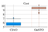
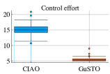
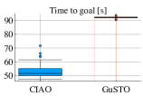
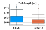
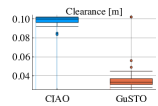
Figure 4: Trajectory Optimization Benchmark Results. CIAO finds faster trajectories with higher clearance than GuSTO.

To evaluate CIAO in terms of planning efficiency and final trajectory quality, we compare it against a set of baselines. We challenge CIAO by using nonlinear dynamics and a nonconvex cost function. Further we use a sampling based motion planner to initialize it with a collision free path that does not satisfy the robot’s dynamics. In this case a NLP-solver is required to solve the CIAO-NLP (1). We use the primal-dual interior point solver Ipopt [29] with the linear solver MA-27 [30] called through CasADi [31] (version 3.4.5).

For the evaluation, we consider three types of experiments:

• numerical experiments to investigate the behavior of the free ball constraint against competing formulations;

• a trajectory optimization benchmark to evaluate the quality of trajectories found by CIAO;

• real-world experiments where CIAO is qualitatively compared to a state of the art baseline.

VI-A Comparison of constraint formulations

In a first set of experiments, the numerical performance of the free ball constraint formulation, as derived in Sec. IV-A, is compared to common alternatives: the actual constraint as defined in Eq. (2) (actual), a linearization of the actual constraint (linear), and a log-barrier formulation (log-barrier). They differ only in the way the obstacle avoidance constraint (IV) is formulated. Our findings are reported in Tab. 2.

	actual	linear	CIAO	log-barrier
ms / iteration	2.00	0.72	0.70	2.23
ms / step	40.78	13.13	17.26	50.34
iterations / step	20.35	18.23	24.64	22.57
time to goal [s]	14.35	14.39	18.67	(13.46)∗
path length [m]	10.22	10.33	10.58	(9.25)∗
max ms / step	448.94	230.07	179.26	$>1000$
% timeouts	0	0	0	11.3

TABLE I: Comparison of constraint formulations.

The average computation time taken per MPC-step and per Ipopt iteration are given as ‘ms / step’ and ‘ms / iteration’ respectively, ‘iters / step’ are the average Ipopt iterations per MPC-step. The path quality is evaluated in terms of ‘time to goal‘ and ‘path length‘. Averages in the first five rows are taken over $62$ scenarios, for which the maximum CPU time of $1.0\rm{s}$ was not exceeded. The percentage of runs that exceed the CPU time is given by ‘% timeouts’. The maximum CPU time taken for a single MPC-step is given by ‘max ms / step’.

We observe that the actual constraint is producing both fastest and shortest paths. This path quality comes at comparatively high computational cost. Linearizing the actual constraint reduces the computational effort, while maintaining a high path quality. In contrast to CIAO, linearization is not an inner approximation and can lead to constraint violations that necessitate computationally expensive recovery iterations. This increases the overall computation time significantly and leads to a higher maximal computation time. At the cost of lower path quality, but a similar average computation time, CIAO overcomes this problem by preserving feasibility. This leads to a lower variance in the computation time, and allows for continuous time collision avoidance guarantees. A further advantage, which is relevant in practice, is that CIAO generalizes to not continuously differentiable distance function implementations, e.g. distance fields.

Including the collision avoidance constraint as a barrier term in the objective, i.e. by adding $-\log(d_{\mathcal{O}}(p_{k})-\underline{d})$ to the stage cost $l_{k}$, is an alternative approach to enforce collision freedom. Our results suggest, however, that for our application it is least favorable among the considered options.

VI-B Trajectory Optimization Benchmark

In a second set of experiments CIAO is compared to GuSTO [7] using the implementation publicly provided by the authors. In these experiments we consider a free-flying Astrobee Robot with 12 states and 6 controls, that has to be rotated and traversed from a start position on the bottom front left corner of a $10\times 10\times 10~{}\mathrm{m}$ cube to a goal in the opposite corner. The room between start and goal point is cluttered with $25$ randomly placed static obstacles of varying sizes (between $1$ and $2$ meters). Fig. 1 shows some examples.

The results reported in Tab. II and Fig. 4 were performed in Julia on a MacBook Pro with an Intel Core i7-8559U clocked at $2.7\rm{GHz}$. The SCPs formulated by GuSTO [7] are solved with Gurobi [32]. Both algorithms are provided with the same initial guess, which is computed based on a path found with RRT [33]. We used a horizon of $100~{}\mathrm{s}$ equally split into $250$ steps, resulting in a sampling time of $0.4~{}\mathrm{s}$.

measure	CIAO	GuSTO
Compute [s]	14.792$\pm$11.966	131.367$\pm$130.743
Iterations	30.660$\pm$15.886	4.520$\pm$1.282
Compute / Iteration [s]	0.475$\pm$0.230	27.729$\pm$22.096
Linearization Error	4.66e-14$\pm$3.67e-15	4.10e-06$\pm$1.28e-06

TABLE II: Numerical Performance: Average $\pm$ std values.

Since both GuSTO and CIAO use tailored cost functions we evaluate the computed trajectories using a common cost function $J_{\rho}$, which is based on the state distance metric $\rho:R^{n_{\mathrm{\mathbf{x}}}}\times R^{n_{\mathrm{\mathbf{x}}}}\to\mathbb{R}$ proposed by [34]: $J_{\rho}(\mathbf{w};\mathbf{x}_{\mathrm{G}})=\sum_{k=0}^{N}\rho(\mathbf{x}_{k},\mathbf{x}_{\mathrm{G}})$, with goal state $\mathbf{x}_{\mathrm{G}}$ and all weights of the distance metric chosen equal. The controls are evaluated separately and reported as control effort given by $J_{\mathrm{\mathbf{u}}}(\mathbf{w})=\sum_{k=0}^{N-1}\Delta t\cdot\left\lVert\mathbf{u}_{k}\right\rVert_{1}$. The path quality is evaluated in terms of time to goal, path length, and clearance (minimum distance to the closest obstacle along the trajectory). The first two measures take the time and path length until the state distance metric falls below a threshold of $0.5$, while the latter is evaluated on the entire trajectory. These three metrics are evaluated on an oversampled trajectory using a sampling time $\Delta t=0.01\,\mathrm{s}$.

The results in Fig. 4 show that CIAO finds faster trajectories than GuSTO and thereby also achieves significantly lower cost. As depicted in Fig. 1 it maintains a larger distance to obstacles for higher speeds. This behavior allows for a higher average speed, at the cost of a higher control activation and slightly longer paths in comparison to GuSTO.

In our experiments both CIAO and GuSTO find solutions to all considered scenarios. As reported in Tab. II, CIAO (Alg. 2) requires more iterations to converge, but the individual iterations are cheaper. Moreover CIAO obtains a feasible trajectory after the first iteration and therefore could be terminated early, while GuSTO does not have this property and takes several iterations to find a feasible trajectory. Even though the dynamics are mostly linear we observe linearization errors for GuSTO, originating from the linear model they use.

In summary CIAO finds trajectories of higher quality than GuSTO at lower computational effort.

VI-C Real-World Experiments - Differential Drive Robot

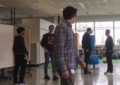
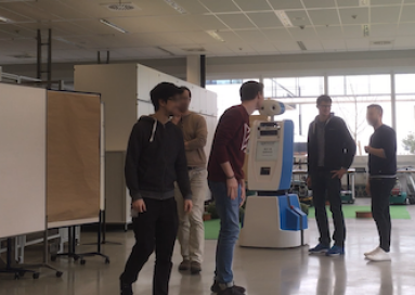
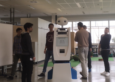
Figure 5: CIAO steers a wheeled mobile robot through a group of people. Real-world (top) and RViz (bottom): Planned trajectory as blue line, free balls as transparent circles, obstacles in yellow, safety margin in light blue.

To qualitatively assess the behavior of CIAO-NMPC (Alg. 3), it was tested in dynamic real-world scenarios with freely moving humans. A representative example is depicted in Fig. 5. Note that CIAO has no knowledge of the humans’ future movements. It is instead considering all humans as static obstacles in their current position.

As in Sec. VI-A a differential drive robot is used, this time with a horizon of $5\,\mathrm{s}$ and a control frequency of $10~{}\mathrm{Hz}$ resulting in a total of $405$ optimization variables (including slacks). For these experiments CIAO was implemented as a C++ ROS-module, the distance function was realized as distance field based on the code by [35]. Initial guesses and reference paths were computed using an A* algorithm [36].

Since GuSTO is not suitable for receding horizon control (RHC), we used an extended version of the elastic-band (EB) method [1]. To obtain comparable results, we used the same A* planner and localization method with both algorithms.

In Fig. 5, it can be seen that the free balls (FBs) (transparent circles) keep to the center of the canyon-like free space. The predicted trajectory (blue line) is deformed to stay inside the FBs. This is a predictive adaptation to the changed environment. For the shown, representative example in Fig. 5 the robot passed smoothly the group. Comparable scenarios were solved similarly by EB.

We observed that groups of people pose a particular challenge that could, however, be solved by both approaches. We note that the robot is moving a bit faster in proximity to people for EB, while CIAO adjusts to blocked paths a bit faster. The most significant difference between the methods is that CIAO combines rotation and backward/forward motion, while the EB rotates the robot on the spot. Both methods succeeded in steering the robot through the group safely, without a single collision.

Figure 6: NLP-solver times obtained in a simulated environment including non-deterministically moving humans. A comparison of these computation times with the ones reported in [7] indicates, that CIAO is computationally cheaper than GuSTO.

Fig. 6 shows representative computation times obtained in simulation on a set of 14 scenarios involving non-deterministically moving virtual humans. The reported computation time accounts only for solving the CIAO-NLP and function evaluations in CasADi, the processing time required by preprocessing steps and other components is not included. High computation times originate from far-from-optimal initializations occurring when a new goal is set, i.e. around time $t=0$, or if humans cross the planned path.

In summary CIAO and the elastic band (EB) approach show similar behavior. In contrast to EB, CIAO computes kinodynamically feasible and guaranteed continuous time collision free trajectories. Further it has a notion of time for the planned motion, such that predictions for dynamic environments can be incorporated in future work.

VII CONCLUSIONS AND FUTURE WORK

This work proposes CIAO, a new framework for trajectory optimization, that is based on a novel constraint formulation, that allows for NMPC based collision avoidance in real-time. We show that it reaches or exceeds state of the art performance in trajectory optimization at significantly lower computational effort, scales to high dimensional systems, and that it can be used for RHC style MPC of mobile robots in dynamic environments.

Future research will focus on extending CIAO to full body collision checking, guaranteed obstacle avoidance in dynamic environments, time optimal motion planning, and multi body robots. A second focus will lie on efficient numerical methods that exploit the structure and properties of the CIAO-NLP stated above.

References

- [1] S. Quinlan and O. Khatib, “Elastic bands: Connecting path planning and control,” in IEEE Int. Conf. Rob. Autom. (ICRA), vol. 2, 1993, pp. 802–807.
- [2] O. Brock and O. Khatib, “Elastic strips: A framework for motion generation in human environments,” Int. J. Rob. Res., vol. 21, no. 12, pp. 1031–1052, 2002.
- [3] M. Zucker, N. Ratliff, A. D. Dragan, M. Pivtoraiko, M. Klingensmith, C. M. Dellin, J. A. Bagnell, and S. S. Srinivasa, “CHOMP: Covariant Hamiltonian Optimization for Motion Planning,” Int. J. Rob. Res., vol. 32, no. 9–10, pp. 1164–1193, 2013.
- [4] J. Schulman, Y. Duan, J. Ho, A. Lee, I. Awwal, H. Bradlow, J. Pan, S. Patil, K. Goldberg, and P. Abbeel, “Motion planning with sequential convex optimization and convex collision checking,” Int. J. Rob. Res., vol. 33, no. 9, pp. 1251–1270, 2014.
- [5] S. L. Herbert, M. Chen, S. Han, S. Bansal, J. F. Fisac, and C. J. Tomlin, “FaSTrack: a modular framework for fast and guaranteed safe motion planning,” in IEEE Conf. Decis. Control (CDC), 2017, pp. 1517–1522.
- [6] X. Zhang, A. Liniger, and F. Borrelli, “Optimization-based collision avoidance,” arXiv preprint arXiv:1711.03449, 2017.
- [7] R. Bonalli, A. Cauligi, A. Bylard, and M. Pavone, “GuSTO: Guaranteed Sequential Trajectory Optimization via sequential convex programming,” in IEEE Int. Conf. Rob. Autom. (ICRA), 2019.
- [8] D. Verscheure, B. Demeulenaere, J. Swevers, J. D. Schutter, and M. Diehl, “Time-optimal path tracking for robots: a convex optimization approach,” IEEE Trans. Autom. Control, vol. 54, pp. 2318–2327, 2009.
- [9] Z. Zhu, E. Schmerling, and M. Pavone, “A convex optimization approach to smooth trajectories for motion planning with car-like robots,” in IEEE Conf. Decis. Control (CDC), 2015, pp. 835–842.
- [10] C. Rösmann, F. Hoffmann, and T. Bertram, “Integrated online trajectory planning and optimization in distinctive topologies,” Robotics and Autonomous Systems, vol. 88, pp. 142–153, 2017.
- [11] J. V. Frasch, A. J. Gray, M. Zanon, H. J. Ferreau, S. Sager, F. Borrelli, and M. Diehl, “An auto-generated nonlinear MPC algorithm for real-time obstacle avoidance of ground vehicles,” in Eur. Control Conf. (ECC), 2013, pp. 4136–4141.
- [12] A. Liniger, A. Domahidi, and M. Morari, “Optimization-based autonomous racing of 1:43 scale RC cars,” Optimal Control Applications and Methods, vol. 36, no. 5, pp. 628–647, 2015.
- [13] T. Faulwasser and R. Findeisen, “Nonlinear model predictive control for constrained output path following,” IEEE Trans. Autom. Control, vol. 61, no. 4, pp. 1026–1039, 2016.
- [14] M. Neunert, C. de Crousaz, F. Furrer, M. Kamel, F. Farshidian, R. Siegwart, and J. Buchli, “Fast nonlinear model predictive control for unified trajectory optimization and tracking,” in IEEE Int. Conf. Rob. Autom. (ICRA), 2016, pp. 1398–1404.
- [15] S. Karaman and E. Frazzoli, “Sampling-based algorithms for optimal motion planning,” Int. J. Rob. Res., vol. 30, no. 7, pp. 846–894, 2011.
- [16] L. Palmieri and K. O. Arras, “A novel RRT extend function for efficient and smooth mobile robot motion planning,” in 2014 IEEE/RSJ International Conference on Intelligent Robots and Systems. IEEE, 2014, pp. 205–211.
- [17] L. Palmieri, S. Koenig, and K. O. Arras, “RRT-based nonholonomic motion planning using any-angle path biasing,” in 2016 IEEE International Conference on Robotics and Automation (ICRA). IEEE, 2016, pp. 2775–2781.
- [18] D. Kouzoupis, G. Frison, A. Zanelli, and M. Diehl, “Recent advances in quadratic programming algorithms for nonlinear model predictive control,” Vietnam J. of Math., vol. 46, no. 4, pp. 863–882, 2018.
- [19] J. Borenstein and Y. Koren, “The vector field histogram – fast obstacle avoidance for mobile robots,” IEEE Trans. Rob. Autom., vol. 7, no. 3, pp. 278 – 288, 1991.
- [20] D. Fox, W. Burgard, and S. Thrun, “The dynamic window approach to collision avoidance,” IEEE Rob. Autom. Mag., vol. 4, no. 1, pp. 23 – 33, 1997.
- [21] N. Y. Ko and R. G. Simmons, “The lane-curvature method for local obstacle avoidance,” in IEEE/RSJ Int. Conf. Intell. Rob. Syst. (IROS), vol. 3, 1998, pp. 1615 –1621.
- [22] P. Fiorini and Z. Shiller, “Motion planning in dynamic environments using velocity obstacles,” Int. J. Rob. Res., vol. 17, no. 7, pp. 760–772, 1998.
- [23] J. Minguez and L. Montano, “Nearness diagram (nd) navigation: Collision avoidance in troublesome scenarios,” IEEE Transactions on Robotics and Automation, vol. 20, no. 1, pp. 45–59, February 2004.
- [24] Y. xiang Yuan, “Recent advances in trust region algorithms,” Mathematical Programming, vol. 151, no. 1, pp. 249–281, June 2015.
- [25] H. G. Bock and K. J. Plitt, “A multiple shooting algorithm for direct solution of optimal control problems,” in Proceedings of the IFAC World Congress. Pergamon Press, 1984, pp. 242–247.
- [26] A. Wächter and L. T. Biegler, “On the implementation of an interior-point filter line-search algorithm for large-scale nonlinear programming,” Mathematical Programming, vol. 106, no. 1, pp. 25–57, 2006.
- [27] L. Palmieri and K. O. Arras, “Distance metric learning for RRT-based motion planning with constant-time inference,” in 2015 IEEE International Conference on Robotics and Automation (ICRA). IEEE, 2015, pp. 637–643.
- [28] L. Palmieri, T. P. Kucner, M. Magnusson, A. J. Lilienthal, and K. O. Arras, “Kinodynamic motion planning on gaussian mixture fields,” in 2017 IEEE International Conference on Robotics and Automation (ICRA). IEEE, 2017, pp. 6176–6181.
- [29] A. Wächter and L. Biegler, “IPOPT - an Interior Point OPTimizer,” https://projects.coin-or.org/Ipopt, 2009.
- [30] HSL, “A collection of Fortran codes for large scale scientific computation.” http://www.hsl.rl.ac.uk, 2011.
- [31] J. A. E. Andersson, J. Gillis, G. Horn, J. B. Rawlings, and M. Diehl, “CasADi: a software framework for nonlinear optimization and optimal control,” Mathematical Programming Computation, 2018.
- [32] Gurobi Optimization, LLC, “Gurobi optimizer reference manual.”
- [33] S. M. LaValle, Planning Algorithms. Cambridge Univ. Press, 2006.
- [34] S. M. LaValle and J. James J. Kuffner, “Randomized kinodynamic planning,” Int. J. Rob. Res., vol. 20, no. 5, pp. 378–400, 2001.
- [35] B. Lau, C. Sprunk, and W. Burgard, “Efficient grid-based spatial representations for robot navigation in dynamic environments,” Robotics and Autonomous Systems, vol. 61, no. 10, pp. 1116–1130, 2013.
- [36] P. E. Hart, N. J. Nilsson, and B. Raphael, “A formal basis for the heuristic determination of minimum cost paths,” IEEE Transactions on Systems Science and Cybernetics, vol. 4, no. 2, pp. 100–107, 1968.