Generating Local Search Neighborhood
with Synthesized Logic Programs

Abstract

Local Search meta-heuristics have been proven a viable approach to solve difficult optimization problems. Their performance depends strongly on the search space landscape, as defined by a cost function and the selected neighborhood operators. In this paper we present a logic programming based framework, named Noodle, designed to generate bespoke Local Search neighborhoods tailored to specific discrete optimization problems. The proposed system consists of a domain specific language, which is inspired by logic programming, as well as a genetic programming solver, based on the grammar evolution algorithm. We complement the description with a preliminary experimental evaluation, where we synthesize efficient neighborhood operators for the traveling salesman problem, some of which reproduce well-known results.

1 Introduction

Size and high dimensionality of the combinatorial problems often make them infeasible for the exhaustive optimization methods, thus giving rise to meta-heuristics — a family of methods aimed at efficiently exploring the search space in pursuit of good enough local optima. Local Search algorithms — well established members of this family — represent the search space in terms of the optimization criterion and a so-called neighborhood operator, which defines a neighborhood relation over the candidate solutions (configurations). A Local Search solver starts with a single configuration and then replaces it with one of its neighbors, repeating this process until the termination condition is met. The high impact of the neighborhood operator choice on the solvers’ performance has induced vast amounts of research on problem-specific operators, which often outperform the generic search strategies [20, 10].

While there has been noticeable recent progress in automated algorithm configuration, including such complicated tasks as finding efficient hyper-parameters [16], feature selection [12] and designing deep neural network architectures [6], there is still no satisfying method to create a problem-specific Local Search strategy. This paper aims at filling this gap by presenting a system capable of inferring Local Search neighborhoods from a fine-grained problem representation consisting in an augmented Constraint Programming model.

Section 3 shortly presents a Neighborhood Description Language [17] — a formalism designed to express neighborhood operators in a declarative manner along with a runtime environment. The rest of the paper is dedicated to synthesizing the aforementioned operators by means of a Grammar Evolution [15] algorithm applied on a Logic Programming DSL tailored to the given optimization problem. The synthesis process is guided by a fitness function which considers both syntax of the generated program and various features of the actual induced neighborhood. We conclude the paper with initial experimental results, conducted on the Traveling Salesman Problem, showing that our system is able to “reinvent” state-of-the-art neighborhood operators.

2 Related Works

Automatic inference of the search algorithm from a CP model was already proposed in [5]. Authors of Comet [18] have proposed method of synthesizing Local Search strategies [19]. The Comet modeling language included mechanisms to independently model both a problems’ structure and the search strategy, including simple neighborhoods. One of the inferred search strategy features was to use neighborhood operators to replace some hard constraints, e.g. the alldifferent constraint. This approach was further proclaimed in [9] and implemented by the Yuck [13] and OscaR/CBLS [4] solvers, providing dedicated neighborhoods to handle specific global constraints. Recently, a system was proposed which infers plausible neighborhood operators from data structures occurring in the Constraint Programming model, as defined in the Essence language  [2]. During the search, the solver switches between those promising neighborhoods using classic multi-arm bandit algorithms. The resulting strategy proved to be superior to or competitive with popular generic strategies on several common combinatorial problems.

3 The NDL Language

All experiments described herein, and their respective results, are founded on a novel method of representing Local Search neighborhood operators called the Neighborhood Definition Language (NDL). NDL uses the underlying CSP (or COP) structure, stated as a Constraint Programming model, to specify a non-deterministic program, capable of inducing a set of new configurations (neighbors) starting from a single point in the search space.

To capture the high-level structure of the considered problem, we have extended the traditional constraint graph representation with labels, which group constraints and variables based on the context of their occurrence in the model. This structure is called the Typed Constraint Graph (or TCG), as the labels are called respectively variable and constraint types:

• variable types $T_{V}=\{t_{1}^{v},t_{2}^{v},\dots t_{n}^{v}\}$ correspond to the indexed data structures, i.e. arrays, commonly used in Constraint modeling languages. Every constraint graph node $v\in V$ is then labeled after its origin array and the index it was defined with: $l_{v}:V\rightarrow\mathbb{I}\times T_{V}$, where $\mathbb{I}$ is a set of array indexes.

• constraint types $T_{C}=\{t_{1}^{c},t_{2}^{c},\dots t_{m}^{c}\}$ capture the relation between constraints which share not only their semantics, but also their origin. We say that constraints share their type if they have been defined by means of a single aggregation function (e.g. quantifier) or they come from decomposition of a single global constraint. Every constraint graph edge $c\in C$ is labeled with its respective type: $l_{c}:C\rightarrow T_{C}$. It is worth mentioning that a Typed Constraint Graph requires global constraints to be decomposed as it supports only binary constraints.

Such a rich problem representation allows NDL programs to query the configuration based both on its semantic and syntactic structure by means of so called selectors. A selector is a non-deterministic operator which can find a set of variables satisfying specified constraints, e.g. variables of a given type, variables constrained by a specific type of constraint. The selected variables may be then tested and accepted by filters — basic arithmetic and logical tests allowing to prune out unwanted variables, based on their values. Finally modifiers are used to perturb a configuration by reassigning new values to a given set of variables. All of these operations may be chained by means of functional composition and result in a first-order non-deterministic program meant to produce sets of neighboring configurations.

First-order NDL programs are limited in terms of expressiveness due to fixed number of variables involved in every operator. To amend this lack, we augment the language with second-order combinators. As in recursion schemes found in functional programming languages [14], combinators perform common primitively recursive computational patterns, lifting the first-order programs to operate sequentially on several different parts of the configuration. There are three combinators available in the language:

• Selector Quantifier applies a program to all possible results of a non-deterministic selector.

• The Least Fixpoint Operator iterates trough the Typed Constraint Graph edges in a breadth-first search manner and applies a given program to the edges nodes.

• Iterator treats a variable as the beginning of an ordered collection where every element is defined by the previous element’s value; then performs the specified program on each of the collection’s elements, similarly to map in functional programming languages.

Due to the problems being of finite size and intrinsically limited recursive nature, all combinators are bound to eventually finish computation, thus eschewing Turing completeness and associated issues. A more detailed list of NDL features and its components can be found on the project wiki and in the language grammar defined in Section 4.1.

3.1 Noodle Runtime

At present, we have one implementation of the NDL language named Noodle, built with the SWI-Prolog [21] system. The core of the Noodle runtime consists of two domain specific languages, Noodle Domain Language (NoodleDL) and Noodle Query Language (NoodleQL) respectively aimed at representing Typed Constraint Graph and NDL programs. Both languages are implemented by means of Prolog meta-programming facilities and are compiled ahead of time to plain Prolog: NoodleDL creates a knowledge base which encodes the problem and NoodleQL is first type checked and then translated to a program which implements the neighborhood operator per se. Figure 1 presents this process in a graphical manner.

The choice of Logic Programming for the NDL implementation was motivated by several unique features. Foremost, NDL depends on non-deterministic evaluation, inherent to Logic Programming in the form of backtracking. Secondly, having the Typed Constraint Graph encoded in the knowledge base, selectors may be efficiently implemented as standard queries, leaving aside various technical issues. Last, but not the least, meta-programming features allowed us to quickly prototype and improve the Noodle DSLs.

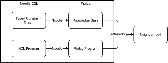
Figure 1: Evaluation of NDL program by the Noodle runtime.

4 Synthesis Algorithm

A common method of synthesizing logic programs entails resorting to an Inductive Logic Programming system, which creates programs given a prior background knowledge and learning examples. In our situation, this approach cannot be applied as there is no learning data available before finishing the synthesis process; in other words, induction would be a viable method to find theories (operators) to define a-priori known neighborhoods, but is unable to generate novel operators. Other possible approaches consist in the application of discrete optimization methods, most notably evolutionary techniques branded as Genetic Programming algorithms. Unfortunately most of those methods tend to be limited in terms of the program representation, often allowing only explicit tree structures as used in the LISP-like languages. Another limitation, critical due to the typed nature of NDL, is the so called type closure — making all values in the synthesized program share a single type.

To address these issues, the NDL framework uses the Grammar Evolution [15] algorithm, a genetic programming method based solely on the formal grammar of the language under consideration paired with an adequate fitness function. We now present a mechanism for translating an NDL problem into a corresponding formal grammar, exploiting structural information present in the model. Next, we will describe various components of the fitness function, together with an experimental evaluation.

4.1 Grammar

As previously stated, we chose to build the NDL framework on a Prolog runtime engine. Knowing this, the grammar which we’ll use to introduce the formal NDL language will be naturally expressible as a Logic program. Every neighborhood operator will thus be represented as a conjunction of atoms:

program atom atom $\land$ program

There are four types of atoms in every program: atom selector modifier filter combinator

Selectors are used to query the NDL model for specific variables, constraints and values occurring in the CSP being represented. The number and shape of the selectors depends therefore on the types existing in the model. Selectors are the sources of the operator: they bring in parts of the CSP, designating sets of constraints, variables or values.

selector $constraint(c,\bnfpn{t1},\bnfpn{t2})\bnfor variable(\bnfpn{i},\bnfpn{t})\\ \bnfor value(\bnfpn{t},\bnfpn{d})\bnfor constant(c,\bnfpn{d})$

Variables in the problem may have their value modified via one of the three available modifiers: set — setting the specified value, swap — swapping two variables’ values and flip — flipping variable’s value between two possible outcomes. Considering variables of type t and domain d:

modifier $set(\bnfpn{t},\bnfpn{d})\bnfor swap(\bnfpn{t},\bnfpn{t})\bnfor flip(\bnfpn{t},\bnfpn{d},\bnfpn{d})$

Filters are used to prune out unwanted results by checking basic properties of the current configuration, e.g. whether a given constraint is satisfied or whether two values are equal.

filter $is\_satisfied(c,\bnfpn{t1},\bnfpn{t2})\bnfor is\_violated(c,\bnfpn{t1},\bnfpn{t2})\\ \bnfor\bnfpn{t}\bnfsp\bnftd{$\neq$}\bnfpn{t}\bnfor\bnfpn{t}\bnfsp\bnftd{$=$}\bnfsp\bnfpn{t}\bnfor\bnfpn{d}\bnfsp\bnftd{$\neq$}\bnfpn{d}\bnfor\bnfpn{d}\bnfsp\bnftd{$=$}\bnfsp\bnfpn{d}\bnfor\bnfpn{d}\bnfsp\bnftd{$<$}\bnfsp\bnfpn{d}$

Our grammar includes three types of second-order atoms for_each, bfs_over and iterate corresponding adequately to Selector Quantifier, The Least Fixpoint Operator and Iterator introduced in Section 3. The only addition are two variations: bfs_over_inverted exploring the constraint graph with inverted arcs and iterate_reversed that treats a given variable as the last element of the considered collection. It is worth mentioning that iterate (and iterate_reversed) may be only used when the variable’s domain and index set coincide:

combinator $for\_each(\bnfpn{selector},\bnfpn{program})\\ \bnfor bfs\_over(c,\bnfpn{t1},\bnfpn{t1}-\bnfpn{t2},\bnfpn{program})\\ \bnfor bfs\_over\_inverted(c,\bnfpn{t2},\bnfpn{t1}-\bnfpn{t2},\bnfpn{program})\\ \bnfor iterate(\bnfpn{t},\bnfpn{t}-\bnfpn{t}),\bnfpn{program})\\ \bnfor iterate\_reversed(\bnfpn{t},\bnfpn{t}-\bnfpn{t}),\bnfpn{program})\\$

Finally, in order to synthesize atoms’ arguments we have to introduce terminals for each variable type in the NDL model. For each NDL type, there are three sets of attributes we’re interested in, those which represent NDL variables (t), indexes (i) and values (d).

t Tt0 Tt1 …TtN
dDd0 Dd1 …DdM
iIi0 Ii1 …IiK

It is worth noting that when a variable’s domain and index set are congruent, the corresponding i and d attributes may also collapse to a single non-terminal.

The basic grammar already covers the core concepts, but it may be augmented with a few features, aiming to make it more expressive:

• Local Scopes — NDL language features local variables bound only in the local scope of a combinator. We partition the sets of non-terminals corresponding to the variables into two sets of global and local, constraining the second one to occur only inside the local scopes.

• Symmetry Breaking — the basic grammar is highly susceptible to a very simple symmetry — variables’ names are only labels and may be permuted, like colors in the graph coloring problem. While BNF grammars can not impose any order on the used non-terminals, some of the variables still may be fixed in certain situations, e.g. in the first atom of the program.

• Limited Depth — the presented grammar allows one to synthesize nested combinators, leading to arbitrarily large and thus slow programs. In order to prevent this behavior, one can prohibit such nested combinators at the grammar level.

4.2 Fitness Function

Given the formal grammar, we are able to synthesize syntactically correct neighborhood operators. Every generated program is then evaluated by the Noodle runtime, resulting in several metrics which may later be used by the genetic algorithm’s fitness function. The evaluation is done in two phases:

Static Code Analysis

Before executing a program, Noodle performs static analysis on the code, identifying semantically incorrect or unused atoms. Such atoms are treated as ineffective (so called ‘introns’) and are removed from the code only for time of execution. This has beneficial effect both on the execution phase, which does not have to consider runtime errors, and for the genetic algorithm itself as introns are believed to improve the algorithm’s efficiency [3].

This phase results in four metrics:

• used outputs ratio $\textit{R}_{o}\in\left(0,1\right)$, i.e. the number of atoms (e.g. selectors) whose outputs are used by another term.

• provided inputs ratio $\textit{R}_{i}\in\left(0,1\right)$, i.e. the number of correctly used atoms that require input variables to be bound (e.g. filters and modifiers).

• unique arguments ratio $\textit{R}_{u}\in\left(0,1\right)$ counting atoms with no repeating arguments.

• effective atoms ratio $\textit{R}_{e}\in\left(0,1\right)$ is the most “global” metric — it relates to number of atoms that have any effect on the configuration, either directly (by being a properly stated modifier) or indirectly (by providing input to a modifier).

All code related metrics pertain to the number of possible errors and, in the best case scenario, will have value $1$ to indicate the inexistence of any issues. We decided to use a basic fitness function, equal to arithmetic average of the above metrics:

$$\phi_{\textit{code}}=\left(\textit{R}_{o}+\textit{R}_{i}+\textit{R}_{u}+\textit{R}_{e}\right)/4$$

It is worth noting that while this $\phi_{\textit{code}}$ does not say anything about the neighborhood itself, it guides the search process into areas containing a higher density of ‘healthy’ individuals (correct programs.) This has a positive impact, especially on the early generations, which otherwise contain mostly random and incorrect programs.

Neighborhood Analysis

After pruning out the introns, the neighborhood operator is compiled to an executable program which is applied on a testing configuration, in order to sample its neighborhood $N=\left\{n_{0},n_{1},\dots,n_{k}\right\}$. For every neighbor $n\in N$ we calculate two types of partial metrics:

• changes ratio $\textit{R}_{\textit{ch}}:N\rightarrow\left(0,1\right)$, which accounts for the number of differences (variables with different values) between $n$ and the initial configuration.

• satisfied constraints ratio $\textit{R}_{\textit{sat}}:N\times T_{C}\rightarrow\left(0,1\right)$, that counts the satisfied constraints for a specific constraint type, in neighbor $n$. It is computed for every constraint type in the model.

Those values are then accumulated into four neighborhood metrics:

• Size of the neighborhood $s=|N|$.

• Number of unique neighbors $u\leq s$.

• Statistics on introduced changes: $ch_{min}$, $ch_{max}$, $ch_{avg}$, $ch_{stdev}$, respectively the minimum, maximum, average and standard deviation of set $\{R_{ch}(n)\mid n\in N\}$.

• Statistics on satisfied constraints: $sat_{min}^{t}$, $sat_{max}^{t}$, $sat_{avg}^{t}$, $sat_{stdev}^{t}$, respectively the minimum, maximum, average and standard deviation of set $\{R_{sat}(n,t)\mid n\in N\}$, for every constraint type $t\in T_{C}$.

As there are many ways to evaluate a neighborhood, we propose several candidate measures based on the metrics we just presented. The following functions were designed to promote neighborhoods that keep Local Search in a search sub-space which preserves the admissibility of configurations, i.e. one that keeps all the constraints satisfied. Another motivation is to find diversified neighborhoods, with a reasonable proportion of unique configurations:

• size score $\phi_{\textit{size}}=\frac{1}{1+e^{\alpha_{s}\times(-u+\beta_{s}/2)}}$, which promotes larger neighborhoods, but flattens after a specified point due to the logistic function; in our experimentation, parameters $\alpha_{s}=0.5$ resulted in a good slope and $\beta_{s}=\frac{|V|!}{2\times(|V|-2)!}$ has been used to promote neighborhood operators which manipulate at least two different variables.

• ratio of unique neighbors vs. total neighborhood size $\phi_{\textit{unique}}=\frac{u}{s}$. This function penalizes neighborhoods which contain many duplicates.

• normalized mean squared satisfiability score $\phi_{\textit{NMSS}}=\frac{\sum\limits_{t\in T_{C}}(sat_{min}^{t})^{2}}{|T_{C}|\times|V|\times chg_{avg}}$, which rewards neighborhoods in proportion to the number of satisfied constraints for each constraint type. It is normalized against the number of changes in the neighborhood, to prevent bias toward operators which don’t introduce any changes to the configuration.

• satisfiability score $\phi_{\textit{sat}}=\frac{\sum\limits_{t\in T_{C}}score(t)}{|T_{C}|}$, which rewards the neighborhoods that satisfy as many constraints as possible. The following $score$ function is designed to prefer neighborhoods that contain even single promising neighbors:

  $$\textit{score}(t)=\begin{cases}sat_{min}^{t}=1,&1\\ {otherwise},&\frac{sat_{max}^{t}}{|V|}\end{cases}$$

• variability score $\phi_{\textit{var}}=\frac{1}{1+e^{\alpha_{v}\times(-ch_{stdev}+\beta_{v})}}$, which promotes neighborhoods in which configurations differ in a varying number of variables. It may be applied to look after ‘complex’ neighborhood operators. In our experiments, we have set parameters $\alpha_{v}=40$ and $\beta_{v}=0.06$ in order to flatten this function quickly.

5 Experimental Results

In order to evaluate the Noodle framework, we have conducted several experiments of synthesizing neighborhood operators for the Traveling Salesman Problem. This problem has been chosen because of its popularity and vast body of research on efficient local search strategies [11].

5.1 Experimental Setup

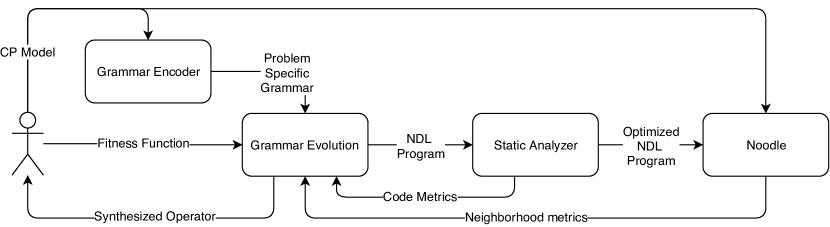
Figure 2: Experiment architecture.

Grammar Evolution can be tuned using various hyper-parameters specific to the genetic programming algorithms. The results we present here were achieved using default settings, leaving the issue of hyper-parameter tuning for future work. The diversity of the synthesized operators stems from the different fitness functions used in the generation process. Every result presented herein was achieved with the following fixed hyper-parameter values:

• population size equal to 1000 and elite pool of size 10;

• 50 generations;

• subtree cross-over operator with probability 0.75;

• subtree mutation operator applied 2 times to every individual;

• tournament selection strategy of size 2;

• PI-grow [7] initialization method;

• generated syntax tree limited to maximum depth 90.

Experiments were conducted on a Debian machine, featuring four 16-core Opteron 6376 CPUs and 128GB ECC RAM. Effectively, it allowed to evaluate the population in parallel with 64 separate processes. On the software side, a 4.9.130 Linux kernel has been used, together with Grammar Evolution implemented by the current development version of the PonyGE2 framework [8] (commit 06b1a8c) running on top of CPython 3.5.3. Figure 2 (on page 2) presents the flow of data in the experiment.

5.2 Problem Representation

All experiments were conducted using the standard Constraint Programming representation of the TSP problem based on the circuit global constraint, defined over an array of next variables, corresponding to the list of edges making up the TSP route. Compared to the more basic alldifferent constraint, this one reveals more information about the problem structure.

As NDL supports only binary constraints, the global constraint circuit had to be decomposed by adding an additional array of variables order, representing the cities visited in the order defined by the edges, starting at the first city:

$$\textit{order}[i]=\begin{cases}i=1,&1\\ i>1,&next[order[i-1]]\end{cases}$$

It is worth noting that it is unnecessary to handle the order variables explicitly, as they depend directly on the next array. The Noodle framework updates the values of such variables during constraint propagation and, at the moment, they are not accessible from the neighborhood operator itself.

There are three types of constraints involved in the problem decomposition. Assuming that $\mathbb{I}$ is a set of city indexes:

• all_diff_next — every pair of the next variables has to be different:

  $$\forall i,j\in\mathbb{I}:i\neq j\implies next[i]\neq next[j]$$

• all_diff_order — every pair of the order variables has to be different:

  $$\forall i,j\in\mathbb{I}:i\neq j\implies order[i]\neq order[j]$$

• self_diff_next — a redundant unary constraint preventing self-loops by stating that variable of type next should not point at itself:

  $$\forall i\in\mathbb{I}:\textit{next}[i]\neq i$$

While all the constraints take part in the fitness function as explained in Section 4.2, all_diff_next may be also used to explore the constraint graph via the Least Fixpoint Operator combinator introduced in Section 3. As next variables use the same set of values for both domain and index set, they make take part in the Iterator combinator, and may be encoded with only two sets of terminals: $\{$T0, T1, …$\}$ representing the variables and $\{$D0, D1, …$\}$ representing both indexes and values.

The evaluation instances used in the experiment consisted of two basic TSP problems, containing respectively six and seven cities, and four admissible solutions, two per problem.

5.3 Synthesized Neighborhood Operators

(a)

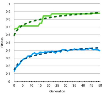
(a)

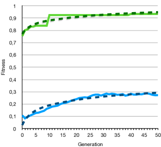
(b)

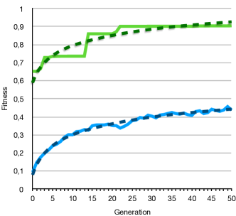
(c)

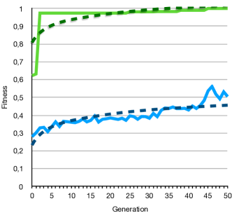
(d)

Figure 3: Fitness improvement during synthesis process. All plots were normalized into $(0,1)$ range.

The experiments we carried out were designed to examine the impact of various fitness functions on synthesis performance and locally optimal neighborhood operators. It turned out we were able to synthesize four distinct interesting operators — two of which already known in the literature as 2-opt and 3-opt [11] and two others which, to the best of our knowledge, lack a proper name and were first time baptized in this paper. Figure 3 shows how fitness of the population progressed during the evolutionary synthesis process of each operator. The noticeable gap between best and average fitness is explained by the destructive influence of the genetic operators and the replacement strategy being used — most of the individuals in each generation are partly random and happen to be semantically incorrect which leads to very low fitness score for the neighborhood quality. It is also worth noting that, while the average fitness tends to continuously improve, the best individuals change in a more discrete manner and correspond to novel neighborhood operators.

Because of space constraints, we only detail the 2-opt case, resorting to a brief description of the other results.

5.3.1 2-opt Neighborhood

The 2-opt operator is a widely known and efficient neighborhood operator used in the traveling salesman (TSP) and related problems. Given the directed graph representation of the salesman route, there are two steps involved in a single 2-opt move. First, two arcs are removed from the route and replaced with two new arcs, connecting the corresponding source and sink nodes of the original arcs. Afterward, in order to keep the directed graph cyclic, one needs to reverse the direction of a single path connecting the new arcs. There are two important properties to this process:

• it keeps the configuration admissible, i.e. if the initial configuration was a Hamiltonian cycle, this will remain true for the neighbor configuration.

• the number of reassigned variables varies with the choice of the removed edges.

The fitness function we used in order to synthesize the 2-opt operator was designed as the following weighted sum:

$$\Phi_{\textit{2-opt}}=\phi_{\textit{code}}+2\times\left(\phi_{\textit{NMSS}}+\phi_{\textit{sat}}+\phi_{\textit{size}}\times\phi_{\textit{unique}}\times\phi_{\textit{var}}\right)$$ (1)

Where the fitness components $\phi$ were defined in Section 4.2 and $\Phi_{\textit{2-opt}}\in\left(0,7\right)$. The $\phi_{\textit{unique}}$ component plays a crucial role as it penalizes neighborhood operators with a constant number of reassigned variables, like the basic 3-opt operator described in the Section 5.4.

Listing 1 contains the 2-opt operator as synthesized by the Noodle framework. It is worth noting that lines 2 and 3 do not have any impact on the inferred neighborhood (variables T2, D1, D3 are not connected to any proper modifier). As previously mentioned (see Section 4.2)) they are treated as introns and therefore get pruned away before the evaluation. Line 4 is also an intron, but for a different reason — the D2 variable is not bound at the time and the whole comparison would lead to a run-time exception. A simplified version of the same operator is shown in Listing 2: it is this code that is tested against the fitness function. Still, even when pruned out, introns leave a negative impact on the $\phi_{\textit{code}}$ fitness component.

⬇

1. constraint(all_diff_next, T0, T1) $\land$

2. variable(D1, T2) $\land$

3. variable(D3, T2) $\land$

4. D2 < D3 $\land$

5. iterate(T0, T3 - T4,

5.1 constraint(all_diff_next, T4, T1) $\land$

5.2 swap_values(T1, T0) $\land$

5.3 swap_values(T4, T0))

Listing 1: 2-opt Neighborhood operator synthesized by the Noodle framework.

⬇

1. constraint(all_diff_next, T0, T1) $\land$

2. iterate(T3 - T4, T0, (

2.1 constraint(all_diff_next, T4, T1) $\land$

2.2 swap_values(T1, T0) $\land$

2.3 swap_values(T4, T0)))

Listing 2: 2-opt operator after removing introns and singleton variables.

Remarkably, the synthesized operator does not resemble any common 2-opt implementation and requires an explanation on its workings. As in the classic 2-opt we can split the process in two parts (line numbers refer here to Listing 2):

1. Line 1 binds NDL variables T0 and T1 to two problem variables involved in a all_diff_next constraint. Effectively, this selects two different variables corresponding to two distinct nodes from the TSP route.

2. Line 2 iterates through the next variables starting from T0:

   • Line 2.1 states that iteration will continue only if variables T4 and T1 are connected with the all_diff_next constraint, i.e. only when they are different variables (it means the same as T4 \= T1).

   • Line 2.2 swaps the values of T0, and T1, effectively removing two arcs from the route, and reassembling it into two sub-routes.

   • Line 2.3 creates a new route from the sub-routes created in the previous step.

   • The iterator goes through all the edges in the path connecting T0 and T1; then terminates due to the line 2.1 being unsatisfied, i.e. because T4 = T1.

Figure 4 presents effects of the synthesized 2-opt operator, performed on a simple 6-node traveling salesman route.

(a)

(b)

(c)

(d)

(e)

(f)

Figure 4: Sequence of consecutive configurations in the 2-opt neighborhood as defined in Listing 2.

5.4 Other Results

We synthesized three other neighborhood operators: basic 3-opt, even swap and 3-swap.

Basic 3-opt

is a simplified operator from the 3-opt family; one that not requires reversing any path in the graph. Given two different next variables T0, T1 and T2 being T1’s successor, their values gets swapped such that to T0 is assigned an old value of T1, to T1 value of T2 and to T2 value of T0. This operator is a strong attractor when the fitness function does not reward operators with a varying amount of changes:

$$\Phi_{\textit{3-opt}}=\phi_{\textit{code}}+2\times\left(\phi_{\textit{NMSS}}+\phi_{\textit{sat}}+\phi_{\textit{size}}\times\phi_{\textit{unique}}\right)$$ (2)

Even swap

is a very simple neighborhood operator that keeps the solution admissible only when the route length is even. Starting at a single next variable T0, it iterates backwards over other variables, swapping values of T0 and its predecessors. Every odd swap breaks the route into two independent cycles and every even swap reassembles them back into a whole. Given the even number of the variables, the process always ends with an admissible configuration, quite different from the initial one. This operator was synthesized as a result of over-fitting to the test data containing only routes of even length. The fitness function being used was the same as in the 3-opt case.

3-swap

is a complex operator composed of two operators: basic 3-opt and an even swap, improved with checks to work on routes of any length. This operator is a result of over-fitting due to the amount of features included in the fitness function:

$$\Phi_{\textit{3-swap}}=\phi_{\textit{code}}+2\times( \phi_{\textit{NMSS}}+\phi_{\textit{sat}}+0.6\times\phi_{\textit{size}}\times\phi_{\textit{unique}}\times\phi_{\textit{var}}+$$

$$0.1\times\phi_{\textit{size}}\times\phi_{\textit{unique}}+0.1\times\phi_{\textit{unique}}\times\phi_{\textit{var}}+0.1\times\phi_{\textit{size}}\times\phi_{\textit{var}}+$$

$$0.05\times\phi_{\textit{size}}+0.05\times\phi_{\textit{amount}})$$

6 Conclusion

In this paper we have presented a program synthesis framework capable of finding problem-specific Local Search neighborhoods based on the Constraint Programming model structure. To achieve this goal, a novel neighborhood representation scheme, called Neighborhood Description Language or NDL, has been introduced. We have shown that NDL statements may be compiled to Prolog code and executed by means of Noodle runtime. To synthesize the NDL programs, a Grammar Evolution algorithm has been proposed along with adequate fitness functions and a method for creating admissible formal grammars. The system described herein has been evaluated on the Traveling Salesman Problem (TSP) and proved able of reproducing efficient neighborhood operators, commonly used among the optimization community, among others.

We plan to research and experiment so as to cover other discrete optimization problems, including domains with no known efficient Local Search strategy. It will require more detailed insight into the involved hyper-parameters and the algorithm configuration methods. All the novel results, including TSP neighborhoods presented in this paper, need to be analyzed in terms of their runtime solving efficiency, using public test instances. Such evaluation may be interleaved with the synthesis process, guiding it further into promising search space areas.

References

- [1]
- [2] Özgür Akgün, Saad Attieh, Ian P. Gent, Christopher Jefferson, Ian Miguel, Peter Nightingale, András Z. Salamon, Patrick Spracklen & James Wetter (2018): A Framework for Constraint Based Local Search using Essence. In: Proceedings of the Twenty-Seventh International Joint Conference on Artificial Intelligence, IJCAI-18, International Joint Conferences on Artificial Intelligence Organization, pp. 1242–1248, 10.24963/ijcai.2018/173.
- [3] Peter J. Angeline (1994): Genetic programming and emergent intelligence. In Kenneth E. Kinnear, Jr., editor: Advances in Genetic Programming, MIT Press, Cambridge, MA, USA, pp. 75–97. Available at http://dl.acm.org/citation.cfm?id=185984.185992.
- [4] Gustav Björdal, Jean-Noël Monette, Pierre Flener & Justin Pearson (2015): A constraint-based local search backend for MiniZinc. Constraints 20(3), pp. 325–345, 10.1007/s10601-015-9184-z.
- [5] Samir A. Mohamed Elsayed & Laurent Michel (2011): Synthesis of Search Algorithms from High-Level CP Models. In Jimmy Lee, editor: Principles and Practice of Constraint Programming – CP 2011, Lecture Notes in Computer Science, Springer Berlin Heidelberg, pp. 256–270, 10.1007/978-3-642-23786-7_21.
- [6] Thomas Elsken, Jan Hendrik Metzen & Frank Hutter (2019): Neural Architecture Search, pp. 63–77. Springer International Publishing, Cham, 10.1007/978-3-030-05318-5_3.
- [7] D. Fagan, M. Fenton & M. O’Neill (2016): Exploring position independent initialisation in grammatical evolution. In: 2016 IEEE Congress on Evolutionary Computation (CEC), pp. 5060–5067, 10.1109/CEC.2016.7748331.
- [8] Michael Fenton, James McDermott, David Fagan, Stefan Forstenlechner, Michael O’Neill & Erik Hemberg (2017): PonyGE2: Grammatical Evolution in Python. Proceedings of the Genetic and Evolutionary Computation Conference Companion on - GECCO ’17, pp. 1194–1201, 10.1145/3067695.3082469. Available at http://arxiv.org/abs/1703.08535. ArXiv: 1703.08535.
- [9] Jun He, Pierre Flener & Justin Pearson (2012): Solution Neighbourhoods for Constraint-directed Local Search. In: Proceedings of the 27th Annual ACM Symposium on Applied Computing, SAC ’12, ACM, New York, NY, USA, pp. 74–79, 10.1145/2245276.2245294.
- [10] Tiago Januario & Sebastián Urrutia (2016): A new neighborhood structure for round robin scheduling problems. Computers & Operations Research 70, pp. 127–139, 10.1016/j.cor.2015.12.016.
- [11] David S. Johnson & Lyle A. McGeoch (1997): The traveling salesman problem: A case study in local optimization. In E. H. L. Aarts & J. K. Lenstra, editors: Local Search in Combinatorial Optimization, John Wiley and Sons, Chichester, United Kingdom, pp. 215–310.
- [12] A. Kaul, S. Maheshwary & V. Pudi (2017): AutoLearn — Automated Feature Generation and Selection. In: 2017 IEEE International Conference on Data Mining (ICDM), pp. 217–226, 10.1109/ICDM.2017.31.
- [13] Michael Marte (2017): Yuck is a constraint-based local-search solver with FlatZinc interface. Available at https://github.com/informarte/yuck. Accessed 2019/05/13.
- [14] Erik Meijer, Maarten Fokkinga & Ross Paterson (1991): Functional programming with bananas, lenses, envelopes and barbed wire. In John Hughes, editor: Functional Programming Languages and Computer Architecture, Springer Berlin Heidelberg, Berlin, Heidelberg, pp. 124–144, 10.1007/3540543961_7.
- [15] Michael O’Neil & Conor Ryan (2003): Grammatical Evolution. In: Grammatical Evolution, Genetic Programming Series, Springer, Boston, MA, pp. 33–47, 10.1007/978-1-4615-0447-4_4.
- [16] B. Shahriari, K. Swersky, Z. Wang, R. P. Adams & N. de Freitas (2016): Taking the Human Out of the Loop: A Review of Bayesian Optimization. Proceedings of the IEEE 104(1), pp. 148–175, 10.1109/JPROC.2015.2494218.
- [17] Mateusz Ślażyński, Salvador Abreu & Grzegorz J. Nalepa (2019): Towards a Formal Specification of Local Search Neighborhoods from a Constraint Satisfaction Problem Structure. In: Proceedings of the Genetic and Evolutionary Computation Conference Companion, GECCO ’19, ACM, New York, NY, USA, pp. 137–138, 10.1145/3319619.3321968.
- [18] Pascal Van Hentenryck & Laurent Michel (2005): Constraint-Based Local Search. The MIT Press.
- [19] Pascal Van Hentenryck & Laurent Michel (2007): Synthesis of Constraint-based Local Search Algorithms from High-level Models. In: Proceedings of the 22Nd National Conference on Artificial Intelligence - Volume 1, AAAI’07, AAAI Press, Vancouver, British Columbia, Canada, pp. 273–278.
- [20] Pascal Van Hentenryck & Yannis Vergados (2006): Traveling Tournament Scheduling: A Systematic Evaluation of Simulated Annealling. In J. Christopher Beck & Barbara M. Smith, editors: Integration of AI and OR Techniques in Constraint Programming for Combinatorial Optimization Problems, Lecture Notes in Computer Science, Springer Berlin Heidelberg, pp. 228–243, 10.1007/11757375_19.
- [21] Jan Wielemaker, Tom Schrijvers, Markus Triska & Torbjörn Lager (2012): SWI-Prolog. Theory and Practice of Logic Programming 12(1-2), pp. 67–96, 10.1017/S1471068407003237.