Towards a model independent extraction of the Boer-Mulders function

Abstract

At present, the Boer-Mulders function for a given quark flavour has been extracted from data on semi-inclusive deep inelastic scattering using the simplifying, but theoretically inconsistent, assumption that it is proportional to the Sivers function for each quark flavour. In this paper, using the latest semi-inclusive deep inelastic COMPASS deuteron data on the $\langle\cos\phi_{h}\rangle$ and $\langle\cos 2\phi_{h}\rangle$ asymmetries we extract the collinear $x_{{}_{\!B}}$-dependence of the Boer-Mulders function for the sum of the valence quarks $Q_{V}=u_{V}+d_{V}$ in an essentially model independent way, and find a significant disagreement with the published results. Our analysis also yields interesting information on the transverse momentum dependence of the unpolarized quark distribution and fragmentation functions.

The Boer-Mulders (BM) function is an essential element in describing the internal structure of the nucleon. In a nucleon of momentum $\bf P$, and for a quark with transverse momentum ${\bf k}_{\perp}$, the BM function measures the difference between the number density of quarks polarized parallel and anti-parallel to ${\bf(P\times k_{\perp})}$. Past attempts to extract it from experiment were hindered by the scarcity of data and made the theoretically inconsistent simplifying assumption Barone:2009hw ; Barone:2008tn that for each quark flavour, it is proportional to the better known Sivers function.

In this paper, we show that the new COMPASS data on the unpolarized $\langle\cos\phi_{h}\rangle$ and $\langle\cos 2\phi_{h}\rangle$ asymmetries in semi-inclusive deep inelastic scattering (SIDIS) reactions for producing a hadron $h$ and and its antiparticle $\bar{h}$ at azimuthal angle $\phi_{h}$, allows an essentially model independent extraction of the BM function.

As explained in Christova:2000nz and Christova:2015jsa there is a great advantage in studying difference asymmetries $A^{h-\bar{h}}$, effectively $A^{h}-A^{\bar{h}}$, since both for the collinear and transverse momentum dependent (TMD) functions, only the flavour non-singlet valence quark parton densities (PDFs) and fragmentation functions (FFs) play a role and the gluon does not contribute. On a deuteron target an additional simplification occurs that independently of the final hadron, only the sum of the valence-quark TMD functions $Q_{V}=u_{V}+d_{V}$ enters. In this paper we use SIDIS COMPASS data on a deuteron target, Adolph:2014pwc , and determine the BM TMD function only for $Q_{V}$, but with essentially no model assumptions.

The unpolarized TMD functions for $Q_{V}$ are parametrized in the standard way Anselmino:2011ch ; Christova:2014gva :

$$f_{Q_{V}/p}(x_{{}_{\!B}},k_{\perp}^{2},Q^{2}) = Q_{V}(x_{{}_{\!B}},Q^{2})\,\frac{e^{-k_{\perp}^{2}/\langle k_{\perp}^{2}\rangle}}{\pi\langle k_{\perp}^{2}\rangle}$$ (1)

and

$$D_{h/q_{V}}(z_{h},p_{\perp}^{2},Q^{2})=D_{q_{V}}^{h}(z_{h},Q^{2})\,\frac{e^{-p_{\perp}^{2}/\langle p_{\perp}^{2}\rangle}}{\pi\langle p_{\perp}^{2}\rangle},$$ (2)

where $Q_{V}(x_{{}_{\!B}},Q^{2})$ is the sum of the collinear valence-quark PDFs:

$$Q_{V}(x_{{}_{\!B}},Q^{2})=u_{V}(x_{{}_{\!B}},Q^{2})+d_{V}(x_{{}_{\!B}},Q^{2})$$ (3)

and $D_{q_{V}}^{h}(z_{h},Q^{2})$ are the valence-quark collinear FFs:

$$D_{q_{V}}^{h}(z_{h},Q^{2})=D_{q}^{h}(z_{h},Q^{2})-D_{\bar{q}}^{h}(z_{h},Q^{2}),$$ (4)

$\langle k_{\perp}^{2}\rangle$ and $\langle p_{\perp}^{2}\rangle$ are parameters extracted from a study of the multiplicities in unpolarized SIDIS. There is some controversy in the literature about their values. This study will suggest a resolution of the problem.

The BM function is parametrized in a similar way:

$$\Delta f^{Q_{V}}_{{}_{B\!M}}(x_{{}_{\!B}},k_{\perp},Q^{2})\!=\!\Delta f^{Q_{V}}_{{}_{B\!M}}(x_{{}_{\!B}},Q^{2})\;\sqrt{2e}\,\frac{k_{\perp}}{M_{{}_{B\!M}}}\;\frac{e^{-k_{\perp}^{2}/\langle k_{\perp}^{2}\rangle_{{}_{B\!M}}}}{\pi\langle k_{\perp}^{2}\rangle},$$ (5)

with

$$\Delta f^{Q_{V}}_{{}_{B\!M}}(x_{{}_{\!B}},Q^{2})\!=\!2\,{\cal N}_{{}_{B\!M}}^{Q_{V}}(x_{{}_{\!B}})\,Q_{V}(x_{{}_{\!B}},Q^{2}).$$ (6)

Here the ${\cal N}^{Q_{V}}_{{}_{B\!M}}(x_{{}_{\!B}})$ is an unknown function and $M_{{}_{B\!M}}$, or equivalently $\langle k_{\perp}^{2}\rangle_{{}_{B\!M}}$:

$$\langle k_{\perp}^{2}\rangle_{{}_{B\!M}}=\frac{\langle k_{\perp}^{2}\rangle\,M^{2}_{{}_{B\!M}}}{\langle k_{\perp}^{2}\rangle+M^{2}_{{}_{B\!M}}},$$ (7)

is an unknown parameter.

Since the asymmetries under study involve a product of the BM parton density and the Collins FF, one requires also the transverse momentum dependent Collins function:

$$\Delta^{N}D_{h/u_{V}\uparrow}(z_{h},p_{\perp},Q^{2})\!=\!\Delta^{N}D_{h/u_{V}\uparrow}(z_{h},Q^{2})\,\sqrt{2e}\,\frac{p_{\perp}}{M_{{}_{C}}}\;\frac{e^{-p_{\perp}^{2}/\langle p_{\perp}^{2}\rangle_{{}_{C}}}}{\pi\langle p_{\perp}^{2}\rangle}\,,$$ (8)

where

$$\Delta^{N}D_{h/u_{V}\uparrow}(z_{h},Q^{2})\!=\!2\,{\cal N}^{h/\!u_{V}}_{{}_{C}}(z_{h})\,D_{u_{V}}^{h}(z_{h},Q^{2}).$$ (9)

The quantities ${\cal N}^{h/\!u_{V}}_{{}_{C}}(z_{h})$ and $M_{{}_{C}}$, or equivalently $\langle p_{\perp}^{2}\rangle_{{}_{C}}$:

$$\langle p_{\perp}^{2}\rangle_{{}_{C}}=\frac{\langle p_{\perp}^{2}\rangle\,M_{{}_{C}}^{2}}{\langle p_{\perp}^{2}\rangle+M_{{}_{C}}^{2}}\,,$$ (10)

are known from studies of the azimuthal correlations of pion-pion, pion-kaon and kaon-kaon pairs produced in $e^{+}e^{-}$ annihilation: $e^{+}e^{-}\to h_{1}h_{2}+X$ and the $\sin(\phi_{h}+\phi_{S})$ asymmetry in polarized SIDIS Anselmino:2008jk ; Anselmino:2015sxa ; Anselmino:2015fty .

Besides the BM-Collins contributions to the $\langle\cos\phi_{h}\rangle$ and $\langle\cos 2\phi_{h}\rangle$ unpolarized asymmetries, there exists also a contribution known as the Cahn effect, which involves only the collinear unpolarized PDFs and FFs.

In Christova:2017zxa we showed that for the range of the COMPASS data, evolution effects can be safely neglected, leading to simplified expressions for the $\langle\cos\phi_{h}\rangle$ and $\langle\cos 2\phi_{h}\rangle$ asymmetries.

In the following the measured asymmetries, denoted $A_{UU}^{\cos\phi_{h}}$ and $A_{UU}^{\cos 2\phi_{h}}$ correspond to the definitions used in the COMPASS paper Adolph:2014pwc . $[\,$Note that several different definitions DAlesio:2007bjf of these asymmetries exist in the literature, some of them even in COMPASS publications Bradamante:2007ex $\,]$. They are related to the theoretical functions via:

$$A_{UU}^{\cos\phi_{h},h-\bar{h}} = \sqrt{\frac{\langle k_{\perp}^{2}\rangle}{\langle Q^{2}\rangle(x_{B})}}\,\left\{{\cal N}_{{}_{B\!M}}^{Q_{V}}(x_{{}_{\!B}})\,{\cal C}_{{}_{B\!M}}^{h}+{\cal C}_{Cahn}^{h}\right\},$$ (11)

$$A_{UU}^{\cos 2\phi_{h},h-\bar{h}} = \left\{{\cal N}_{{}_{B\!M}}^{Q_{V}}(x_{{}_{\!B}})\,\hat{\cal C}_{{}_{B\!M}}^{h}+\frac{\langle k_{\perp}^{2}\rangle}{\langle Q^{2}\rangle(x_{B})}\,\hat{\cal C}^{h}_{Cahn}\right\},$$ (12)

where $\langle Q^{2}\rangle(x_{{}_{\!B}})$ is some mean value of $Q^{2}$ for each $x_{{}_{\!B}}$-bin and the coefficients ${\cal C}_{{}_{B\!M}}$, ${\cal C}_{Cahn}$, $\hat{\cal C}_{{}_{B\!M}}$ and $\hat{\cal C}_{Cahn}$ are dimensionless constants given by integrals over various products of the unpolarized or Collins FFs and, crucially, whose values depend on the parameters $\langle k_{\perp}^{2}\rangle$, $\langle p_{\perp}^{2}\rangle$, $M_{{}_{B\!M}}$ and $M_{{}_{C}}$. For a finite range of integration over $P_{T}^{2}$, corresponding to the experimental kinematics, $a\leq P_{T}^{2}\leq b$, they are given by the expressions:

$${\cal C}_{Cahn}^{h} = -2\,\frac{\int dz_{h}\,z_{h}\,[D_{q_{V}}^{h}(z_{h})]S_{1}(a,b;\langle P_{T}^{2}\rangle)/(\eta+z_{h}^{2})^{1/2}}{\int dz_{h}\,[D_{q_{V}}^{h}(z_{h})]\,S_{0}(a,b;\langle P_{T}^{2}\rangle)}$$ (13)

$${\cal C}_{{}_{B\!M}}^{h} = 4e\,\frac{\lambda_{{}_{B\!M}}^{2}\lambda_{{}_{C}}^{2}}{M_{{}_{B\!M}}M_{{}_{C}}}\,\langle p_{\perp}^{2}\rangle$$ (14)

$$\times\frac{\int dz_{h}\,[\Delta^{N}D_{{q_{V}}\!\uparrow}^{h}(z_{h})]\,[\,z_{h}^{2}\lambda_{{}_{B\!M}}\,S_{3}(a,b,\langle P_{T}^{2}\rangle_{{}_{B\!M}})+\,(\eta\lambda_{{}_{C}}-z_{h}^{2}\lambda_{{}_{B\!M}})\,S_{1}(a,b;\langle P_{T}^{2}\rangle_{{}_{B\!M}})]/(z_{h}^{2}\lambda_{{}_{B\!M}}+\eta\lambda_{{}_{C}})^{3/2}}{\int dz_{h}\,[D_{q_{V}}^{h}(z_{h})]\,S_{0}(a,b;\langle P_{T}^{2}\rangle)}$$

$$\hat{\cal C}^{h}_{Cahn} = \frac{2\int dz_{h}\left(z_{h}^{2}/[\eta+z_{h}^{2}]\right)\,[D_{q_{V}}^{h}(z_{h})]\,S_{2}(a,b;\langle P_{T}^{2}\rangle_{{}_{B\!M}})}{\int dz_{h}\,[D_{q_{V}}^{h}(z_{h})]\,S_{0}(a,b;\langle P_{T}^{2}\rangle)}$$ (15)

$$\hat{\cal C}_{{}_{B\!M}}^{h} = -2e\,\frac{\lambda_{{}_{B\!M}}^{2}\lambda_{{}_{C}}^{2}}{M_{{}_{B\!M}}M_{{}_{C}}}\,\langle p_{\perp}^{2}\rangle\;\frac{\int dz_{h}\,[z_{h}\,\Delta^{N}D_{{q_{V}}\!\uparrow}^{h}(z_{h})]/(z_{h}^{2}\lambda_{{}_{B\!M}}+\eta\lambda_{{}_{C}})\,S_{2}(a,b;\langle P_{T}^{2}\rangle)}{\int dz_{h}\,[D_{q_{V}}^{h}(z_{h})]\,S_{0}(a,b;\langle P_{T}^{2}\rangle)}$$ (16)

where, with $\tau=\textrm{either}\,\,\langle P_{T}^{2}\rangle\,\,\textrm{or}\,\,\langle P_{T}^{2}\rangle_{{}_{B\!M}}$,

$$S_{n}(a,b;\tau) = \int_{a}^{b}\,dP_{T}^{2}\,P_{T}^{n}e^{-P_{T}^{2}/\tau}/\tau^{1+n/2}\,.$$ (17)

Here $[D_{q_{V}}^{h}]$ and $[\Delta^{N}D_{{q_{V}}\!\uparrow}^{h}(z_{h})]$ are combinations of the collinear and Collins FFs:

$$[D_{q_{V}}^{h}(z_{h},Q^{2})] = e_{u}^{2}\,D_{u_{V}}^{h}+e_{d}^{2}\,D_{d_{V}}^{h},$$ (18)

$$[\Delta^{N}D_{{q_{V}}\!\uparrow}^{h}(z_{h},Q^{2})] = e_{u}^{2}\,\Delta^{N}D_{{u_{V}}\!\uparrow}^{h}+e_{d}^{2}\,\Delta^{N}D_{{d_{V}}\!\uparrow}^{h}$$ (19)

and

$$\eta=\frac{\langle p_{\perp}^{2}\rangle}{\langle k_{\perp}^{2}\rangle},\quad\lambda_{{}_{C}} = \frac{M_{{}_{C}}^{2}}{\langle p_{\perp}^{2}\rangle+M_{{}_{C}}^{2}},\quad\lambda_{{}_{B\!M}}=\frac{M_{{}_{B\!M}}^{2}}{\langle k_{\perp}^{2}\rangle+M_{{}_{B\!M}}^{2}}\cdot$$ (20)

As mentioned, there is some controversy as to the values of these parameters, with a wide range of values given in literature. The coefficients ${\cal C}_{Cahn}$, ${\cal C}_{{}_{B\!M}}$, $\hat{\cal C}_{Cahn}$, $\hat{\cal C}_{{}_{B\!M}}$ are given in Table 1, grouped together in Sets corresponding to the values of these parameters, with $\rho=-{\cal C}_{{}_{B\!M}}/\hat{\cal C}_{{}_{B\!M}}$.

SET	$~{}\langle k_{\perp}^{2}\rangle~{}$	$~{}\langle p_{\perp}^{2}\rangle~{}$	$~{}M_{{}_{B\!M}}^{2}~{}$	$~{}M_{{}_{C}}^{2}~{}$	${\cal C}_{Cahn}$	$~{}{\cal C}_{{}_{B\!M}}~{}$	$\hat{\cal C}_{Cahn}$	$~{}\hat{\cal C}_{{}_{B\!M}}~{}$	$~{}~{}\rho~{}~{}$
I	0.18	0.20	0.34	0.91	-0.68	2.1	0.31	-0.47	4.4
II	0.18	0.20	0.19	0.91	-0.68	1.8	0.31	-0.40	4.4
III	0.25	0.20	0.34	0.91	-0.77	1.9	0.38	-0.49	3.8
IV	0.25	0.20	0.19	0.91	-0.77	1.4	0.38	-0.39	3.7
V	0.57	0.12	0.80	0.28	-1.2	0.89	0.84	-0.50	1.8

Table 1: ${\cal C}_{Cahn}$, ${\cal C}_{{}_{B\!M}}$, $\hat{\cal C}_{Cahn}$, $\hat{\cal C}_{{}_{B\!M}}$ and $\rho$ calculated for different sets of $\langle k_{\perp}^{2}\rangle$, $\langle p_{\perp}^{2}\rangle$, $M_{{}_{B\!M}}^{2}$ ($M_{{}_{B\!M}}^{2}=M_{{}_{S}}^{2}$ assumed) and $M_{{}_{C}}^{2}$. The parametrizations for the collinear FFs are from AKK’2008 Albino:2008fy , and for Collins functions – for sets I – IV – from Anselmino:2008jk and Anselmino:2015fty , and for set V – from Anselmino:2015sxa and Anselmino:2015fty . The integrations are according to COMPASS kinematics: $0.01\leq P_{T}^{2}\leq 1\,GeV^{2}$ and $0.2\leq z_{h}\leq 0.85$ Adolph:2014pwc .

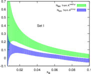
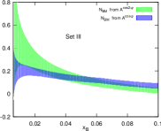
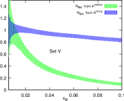
Figure 1: ${\cal N}_{{}_{B\!M}}^{Q_{V}}(x_{{}_{\!B}})$ extracted from the difference asymmetries, Eqs. (11) and (12), using different sets of parameters of Table I. Plots for Sets. II and IV overlap with those for Sets. I and III, respectively.

We form the type of difference asymmetries $A^{h^{+}-h^{-}}_{J}$ advocated in Christova:2017zxa from the corresponding usual asymmetries $A_{j}^{h^{+}}$ and $A_{j}^{h^{-}}$ for positive and negative charged hadron production measured in COMPASS Adolph:2014pwc via the relation Alekseev:2007vi :

$$A_{J}^{h^{+}-h^{-}}=\frac{1}{1-r}\left(A_{J}^{h^{+}}-rA_{J}^{h^{-}}\right),\qquad J=\langle\cos\phi_{h}\rangle,\langle\cos 2\phi_{h}\rangle.$$ (21)

Here $r$ is the ratio of the unpolarized $x_{{}_{\!B}}$-dependent SIDIS cross sections for production of negative and positive hadrons $r=\sigma^{h^{-}}(x_{{}_{\!B}})/\sigma^{h^{+}}(x_{{}_{\!B}})$ measured in the same kinematics Alekseev:2007vi . In practice we construct the difference asymmetries using smooth fits to the data on the usual asymmetries and to the ratio $r$. For $\langle Q^{2}\rangle(x_{{}_{\!B}})$ we perform a linear interpolation of the COMPASS data points.

The relations (11) and (12) provide 2 independent equations for the extraction of ${\cal N}_{{}_{B\!M}}(x_{{}_{\!B}})$ for each set of the parameters in Table I. The results found in Fig.1 show that the 2 extractions are not completely compatible with each other for any choice of the parameters given in Table I. The source of the disagreement, we believe, lies in the value of the Cahn contribution $\hat{\cal C}_{Cahn}$ in Eq. (12). The point is that this Cahn term is a twist-4 contribution and there are certainly other twist-4 contributions, from target mass corrections and other dynamic effects, which we are unable to calculate. One possibility would be to keep only twist-2 terms, but we think it interesting to obtain an estimate of the missing twist-4 terms. We have therefore replaced $\hat{\cal C}_{Cahn}$ by $\hat{\cal C}_{Cahn}+\hat{\cal C}_{1}$ , where $\hat{\cal C}_{1}$ is a free parameter adjusted to improve the compatibility of the two extractions of ${\cal N}_{{}_{B\!M}}^{Q_{V}}$ from Eqs. (11) and (12). We find perfect agreement for the parameter Set I with $\hat{\cal C}_{Cahn}$ replaced by $\hat{\cal C}_{Cahn}+\hat{\cal C}_{1}$ [see Fig. 2] for the following parameter vaues:

$$\langle k_{\perp}^{2}\rangle=0.18,\quad\langle p_{\perp}^{2}\rangle=0.20,\quad M_{{}_{B\!M}}^{2}=0.34,\quad M_{{}_{C}}^{2}=0.91,\quad\hat{\cal C}_{1}=-1.16.$$ (22)

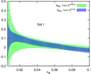
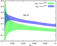
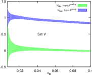
Figure 2: ${\cal N}_{{}_{B\!M}}^{Q_{V}}(x_{{}_{\!B}})$ extracted from the difference asymmetries, Eqs. (11) and (12), using different sets of parameters of Table I and $\hat{\cal C}_{Cahn}+\hat{\cal C}_{1}$ instead of $\hat{\cal C}_{Cahn}$. Again, plots for Sets. II and IV overlap with those for Sets. I and III, respectively.

Note that these values for $\langle k_{\perp}^{2}\rangle$ and $\langle p_{\perp}^{2}\rangle$ agree with those obtained in Giordano:2008th and with the theoretical considerations Zavada:2009ska ; Zavada:2011cv ; DAlesio:2009cps . The value obtained for $\hat{\cal C}_{Cahn}+\hat{\cal C}_{1}=-0.85$ suggests that there are other twist-4 contributions, relatively large compared to the Cahn term, in the $A^{\cos 2\phi,h-\bar{h}}_{UU}$ asymmetry .
An analytic expression for the extracted averaged ${\cal N}_{{}_{B\!M}}^{Q_{V}}$ for the parameter Set given in Eq. (22) is:

$${\cal N}_{{}_{B\!M}}^{Q_{V}}(x_{{}_{\!B}}) = Nx_{{}_{\!B}}^{\alpha}(1-x_{{}_{\!B}})^{\beta}(1+\gamma x_{{}_{\!B}}),$$

$$N=0.475\pm 0.037,\quad\alpha = 0.242\pm 0.022,\quad\beta=13.3\pm 1.7,\quad\gamma=-13.7\pm 0.4\,.$$ (23)

Interestingly, there is a second way to utilize equations (11) and (12) which automatically imposes exact consistency of the extraction of ${\cal N}_{{}_{B\!M}}$, and which more directly fixes the values of the parameters $\langle k_{\perp}^{2}\rangle,\,\langle p_{\perp}^{2}\rangle\,,M_{{}_{B\!M}}$, $M_{{}_{C}}$ and $\hat{\cal C}_{1}$. Eliminating ${\cal N}_{{}_{B\!M}}^{Q_{V}}(x_{{}_{\!B}})$ from Eqs. (11) and (12) and using the variable $\rho$ we obtain:

$$A(x_{{}_{\!B}})=B(x_{{}_{\!B}}),$$ (24)

where

$$A(x_{{}_{\!B}}) \equiv \sqrt{\frac{\langle Q^{2}\rangle(x_{B})}{\langle k_{\perp}^{2}\rangle}}\,A_{UU,d}^{\cos\phi_{h},h^{+}-h^{-}}(x_{{}_{\!B}})\,+\rho\,A_{UU,d}^{\cos 2\phi_{h},h^{+}-h^{-}}(x_{{}_{\!B}}),$$ (25)

$$B(x_{{}_{\!B}}) \equiv {\cal C}_{Cahn}+\rho\,\frac{\langle k_{\perp}^{2}\rangle}{\langle Q^{2}\rangle(x_{B})}\,\hat{\cal C}_{Cahn}.$$ (26)

Fig. 3 compares these two functions for various choices of the parameters in Table I. It is seen that there is excellent agreement (with $\hat{\cal C}_{Cahn}$ replaced by $\hat{\cal C}_{Cahn}+\hat{\cal C}_{1}$) for the values given in Eq. (22).

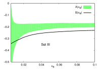
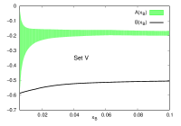
Figure 3: The test of Eq. (24), with $\hat{C}_{Cahn}$ replaced by $\hat{C}_{Cahn}+\hat{C}_{1}$. Again, plots for Sets. II and IV overlap with those for Sets I and III, respectively.

We conclude therefore that the COMPASS data on $A_{UU}^{\cos\phi_{h}}$ and $A_{UU}^{\cos 2\phi_{h}}$ strongly favour the parameter values in Eq. (22). This also confirms our suggestion that there are significant twist-4 contributions other than the Cahn one.

Our valence BM function $\Delta f_{{}_{B\!M}}^{Q_{V}}(x_{{}_{\!B}})$ is shown in Fig. 4, where it is compared to $\Delta f_{{}_{B\!M}}^{Q_{V}}(x_{{}_{\!B}})$ calculated from the BM function published in Barone:2009hw . It is seen that there is a significant difference, suggesting that the BM functions in Barone:2009hw are incorrect. Note, as mentioned earlier, that the extraction in Barone:2009hw is, strictly speaking, theoretically inconsistent.

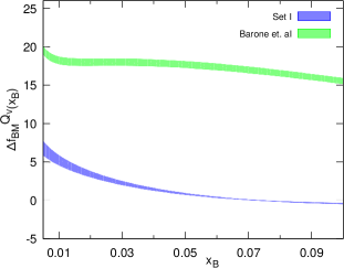
Figure 4: Comparison of $\Delta f_{{}_{B\!M}}^{Q_{V}}$ for Set I, Eq. 22, with the result of Barone et al.Barone:2009hw . We use CTEQ6 parametrization for the collinear PDFs Pumplin:2002vw .

Finally we note that future data on the $\langle\cos\phi_{h}\rangle$ and $\langle\cos 2\phi_{h}\rangle$ asymmetries on protons, for charged pions or kaons, will allow access to the BM function for the valence quarks $u_{V}$ and $d_{V}$ separately, in the same essentially model independent manner Christova:2015jsa .

References

(1) V. Barone, S. Melis and A. Prokudin,
Phys. Rev. D 81, 114026 (2010).
(2) V. Barone, A. Prokudin and Bo-Qiang Ma,
Phys. Rev. D 78, 045022 (2008).
(3) E. Christova and E. Leader, Nucl.Phys. B 607, 369 (2001).
(4) E. Christova and E. Leader, Phys. Rev. D 92, 114004 (2015).
(5) C. Adolph et al. (COMPASS Collaboration),
Nucl. Phys. B 886, 1046 (2014).
(6) M. Anselmino et al., Phys. Rev. D 83, 114019 (2011).
(7) E. Christova, Phys. Rev. D 90 054005 (2014).
(8) M. Alekseev et al. (COMPASS Collaboration),
Phys. Lett B 660, 458 (2008).
(9) M. Anselmino et al., Nucl. Phys. B Proc. Suppl. 191, 98 (2009).
(10) M. Anselmino et al., Phys. Rev. D 92, 114023 (2015).
(11) M. Anselmino et al., Phys. Rev. D 35, 034025 (2016).
(12) E. Christova, E. Leader and M.Stoilov, Phys. Rev. D 97, 056018 (2018).
(13) U. D’Alesio and F. Murgia, Prog. Part. Nucl. Phys. 61, 394 (2008).
(14)
F. Bradamante, AIP Conf. Proc. 915, 513 (2007).
(15) S. Albino, B.A. Kniehl and G. Kramer, Nucl. Phys. B 803, 42 (2008).
(16) F. Giordano, report DESY-THESIS-2008-030
(17) P. Zavada, Phys. Rev. D 83, 014022 (2011).
(18) P. Zavada, Phys. Rev. D 85, 037501 (2012).
(19) U. D’Alesio, E. Leader and F. Murgia, Phys. Rev. D 81, 036010 (2010).
(20) J. Pumplin et al., J. High Energy Phys. 07 (2002) 012.