An axiomatic measure of one-way quantum information
Abstract
I introduce an algorithm to detect one-way quantum information between two interacting quantum systems, i.e. the direction and orientation of the information transfer in arbitrary quantum dynamics. I then build an information-theoretic quantifier of one-way information which satisfies a set of desirable axioms. In particular, it correctly evaluates whether correlation implies one-way quantum information, and when the latter is transferred between uncorrelated systems.
In the classical scenario, the quantity measures information transfer between random variables. I also generalize the method to identify and rank concurrent sources of quantum information flow in many-body dynamics, enabling to reconstruct causal patterns in complex networks.
Keywords: quantum information, quantum correlations, quantum dynamics.
I Introduction
One-way quantum information manifests when the output state of a system in a process is determined by its interaction with another system, but not vice versa. One-way information transfer can be associated to causal relations. A vast literature has discussed the problem of inferring causation from data in both classical and quantum scenarios granger ; massey ; pearl ; shalizi ; rubin ; james ; janzing ; tucci , because of its importance for Science.
Yet, a crucial problem is still unsolved: how can we quantify one-way information between quantum systems? In general, there is no consensus about how to measure the peculiar one-way information flow that characterizes causation. Given the state of a quantum system, measures of quantum correlations mark well the amount of information shared by the components of the system in terms of entropic or geometric quantifiers modirev ; horo . However, given a multipartite quantum channel, we do not have any reliable metric to evaluate the information transferred during its implementation. Unfortunately, widely employed causation measures misinterpret causal links between classical random variables in simple case studies janzing ; james , so we cannot just translate them in the quantum regime.
Here, I construct an information-theoretic measure of one-way information (OWI), capturing the direction of the information flow between causally connected systems. OWI is exemplified by a measuring probe that updates its state based on the information acquired from a measured system. A controlled gate is then an adequate mathematical characterization for OWI flow from a system to another. Another example of OWI is the instruction that a controlling device sends to regulate the state of a controlled machine.
First, I focus on the problem of inferring OWI in an arbitrary quantum channel. I present a three-step algorithm which discovers and evaluates OWI given the input/output states of many-body quantum processes. In other words, it can discriminate different causal relations from same-looking input/output data. Also, it is experimentally implementable with current technology. The scheme builds on previous proposals for evaluating causation chiri ; costa ; chirio ; prx ; chaves ; leifer ; modicaus ; temp ; cava ; shap , which yet did not fully address the problem of quantifying OWI by provably rigorous measures.
Then, I build the OWI quantifier, which is calculated in the output state of the algorithm. I show that the quantity meets a set of important properties, which are not satisfied by widely employed measures in classical information theory. Specifically, it vanishes when there is no information transfer. Unlike correlation quantifiers, it unambiguously pinpoints the source and the recipient of the information. It reliably describes the interplay between correlation and causation, capturing when correlation does imply causation, and when causation exists without correlation. In the classical scenario, it quantifies the amount of information transferred between random variables.
Notably, I show that when the algorithm is run by a quantum computer nielsen , even one of the currently available toy models, can evaluate OWI between classical systems that are untraceable by a classical device which implements an equivalent scheme. Finally, the method is extended to quantify OWI in multipartite systems. I build a measure of conditional causation that satisfies two important properties. First, it localizes the source of information, i.e. the measured system(s), in three or more interacting parties. Second, it ranks multiple concurrent sources in terms of how much they affect, i.e. control, the evolution of a target system. Consequently, it makes possible to quantitatively describe causal patterns in many-body dynamics.
II Quantifier of OWI
An instance of OWI is the coupling of an apparatus with a measured system . The interaction is formalized as a controlled operation . Indeed, the controlled gate is the logic operation related to the pre-measurement step in the ubiquitous Von Neumann meaasurement scheme vn . Here, bits of information flows from to . Consider now the evolution of a bipartite quantum system initially prepared in the state , which is described by the unitary transformation .
Assuming that the channel is unknown, the goal is to quantify how much the dynamics of system influences the dynamics of . The question to answer is then: “How much information transfers to via the channel ?” The task is hard because, given the same initial state, different causal relations can produce the same output. I list two pieces of evidence.
First, the roles of control and target systems are basis-dependent. For example, the two-qubit CNOT is equal to a controlled gate with swapped control and target qubits, and different measurement basis, smolin ; rieffel . The system therefore exerts maximal influence on via the controlled operation only with respect to the bases .
This also implies that calculating the correlations in the input/output states, or the ability of a channel to create correlations zanardi ; luo2 , is insufficient for drawing conclusions on the information flow from a causing device to an affected system.
When the roles of control and target system are inverted, the information travels in the opposite direction, while creating the same amount of correlations.
Second, there can be causal links with neither initial nor final correlations. For example, is a causal relation, conversely to the local bit flip . They are two different physical processes that generate the same output from the same initial state note .
Yet, there is a way to discern OWI from the initial and final states of a quantum process. One can recast the problem of inferring causation in terms of the much better understood task of quantifying correlations, if additional systems are available. I first discuss an illustrative example. Then, I detail a generally applicable scheme.
Suppose one correlates two systems with two auxiliary systems , respectively, such that the global (pure) state is . Consider then three different processes:
| (1) | |||
In the first case, there is no interaction between and , since . The two final controlled operations destroy all the initial correlations. In the second line, instead, a controlled gate generates four-partite correlations by sending information from to . The subsequent controlled gates leave the systems correlated. In the third case, generates a reverse information flow, and correlations between systems survive in the output state. Hence, the direction of the information flow between and , if any, is determined from the correlations in .
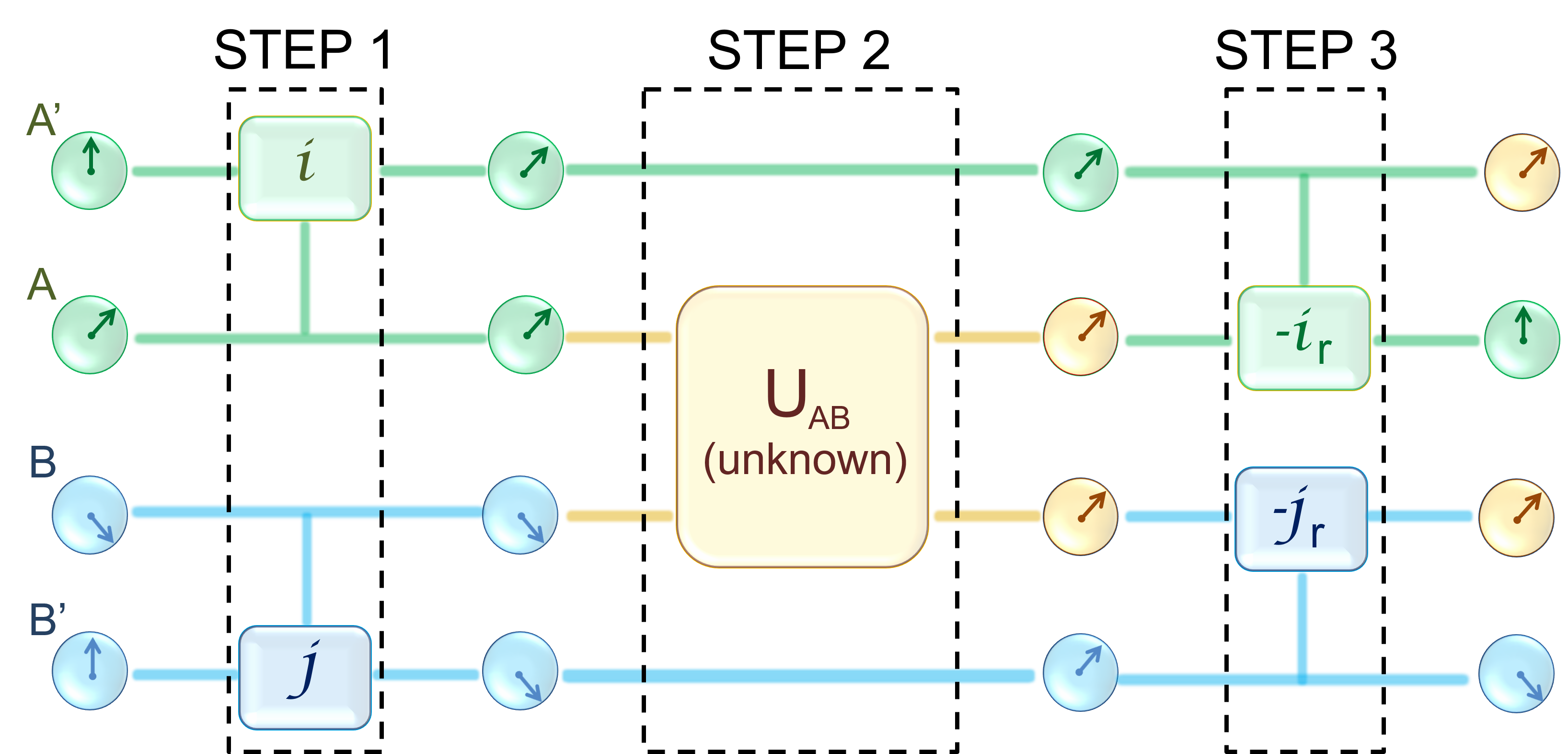
The example suggests a universally valid scheme for quantifying OWI between two -dimensional systems , due to an unknown channel , with respect to reference bases (Fig. 1):
STEP 1 – Given the initial state , with and , apply two controlled operations that create correlations between and two additional systems . Defining , one has
| (2) |
The bases are from now on fixed to be mutually unbiased with respect to the eigenbases of , while the method works for any choice but the eigenbases themselves. For instance, for pure input states, the basis is one in which the input is maximally coherent, , such that the controlled operation creates maximal entanglement with the related auxiliary, , as the initial marginal states of the example. For maximally mixed input states, , one obtains a maximally correlated classical state, .
STEP 2 – Let the system evolve according to the channel ,
| (3) |
STEP 3 (final) – Apply a second pair of local controlled operations with respect to the reference bases , but swapping the roles of control and target systems:
| (4) |
The case study in Eq. 1 implies that one can evaluate the information exchanged by and by calculating the correlations in . The statistical dependence between two systems is quantified by the mutual information in which is the von Neumann entropy of the state . For any third system , the conditional mutual information reads cover . I propose to measure the OWI that sends to via the channel by
| (5) |
which is computed on notanome .
Consequently, the influence of on during the interaction under study is given by .
As a minimal working example, consider two qubits in the input state , and the unitary map to be the CNOT gate . By applying the proposed scheme, one has
As expected, the output state in the example displays correlations between and , . Indeed, causally influences .
III PROOFS THAt the OWI measure satisfies desirable properties, including extension to the multipartite case
To further justify the proposal, I report other explicit calculations for instructive cases in Tables 1, 2. Also, I discuss how the measure meets several desirable properties.
| Process: | ||
|---|---|---|
| 0 | ||
| 0 | ||
| 0 | ||
| Process: | |||
|---|---|---|---|
Information-theoretic consistency. There is no OWI without interaction. For local unitaries ,
one has
. Two systems can influence each other by a two-way information flow, e.g. , with . In such a case, . Yet, the measure is not additive. Given , in general . Indeed, a controlled operation with control and target can be transformed in one with control and target by local unitaries, e.g. , where is the Hadamard gate.
The measure is maximized by a controlled operation with respect to the reference bases and pure input states, . The unitary creates bits of classical correlations between and , and bits of quantum correlations, which are generated by consuming local coherence with respect to the local basis jajun . For a maximally mixed input state, one has , because only bits of classical correlations are created.
Asymmetry. The measure, unlike correlation quantifiers, captures the direction of OWI, . Consider . Evaluating OWI with respect to , one has and . On the other hand, reminding that , the OWI with respect to is and . The measure correctly identifies control (the information source) and target (the affected system).
Quantifying OWI with and without correlations. One of the main challenges in evaluating OWI is discriminating causal links between correlated systems.
The measure defined in Eq. 5 takes zero value for systems that do not exchange information, regardless of the presence of correlations. That is, two correlated systems are left correlated by local unitary channels, but there is no information flow.
A technical caveat is that in the detection scheme the initial correlations between and must be ignored. The input state is , rather than the full state .
A more elusive manifestation of OWI is when there is influence without correlations, e.g. . The measure is able to detect such causal relations, discriminating when is a controlled operation and when the very same input/output transformation is due to a local unitary, . Note that OWI flow is detected even with no state change, e.g. , as the system still receives the instruction “do nothing” from . Indeed, the controlled gate, while generating no change, is a distinct physical process from the identity channel.
Quantifying classical OWI. A measure of OWI transfer between random variables , which overcomes some limitations of previous proposals, is obtained by considering classically correlated input states piani .
The celebrated Granger causality granger , a causation measure widely used in econometrics, is confined to detect linear causal relations. On the same hand, the transfer entropy and the causation entropy infotransfer ; causal , employed in network science, fail to detect causation generated by logic gates, such as the CNOT (XOR) applied to time series, , and the SWAP, james ; janzing . The quantity in Eq. 5 instead correctly describes causal relations implemented by classical gates (see Table 1). For instance, for maximally mixed inputs one has . The result is independent of the chosen decomposition for the SWAP gate in terms of controlled gates swap .
Moreover, a surprising result is obtained: Quantum devices can detect OWI between classical systems that is untraceable by classical machines, if the proposed evaluation scheme is adopted. Consider the process , in which two systems carry information about two random variables.
If is a classical four-bit register, no superpositions with respect to the basis are possible. Applying the method in Fig. 1, the final state is . Hence, no OWI can be detected by classical means. If instead we store the information about the classical variables into the states of two qubits , and the auxiliary are quantum systems as well, quantum correlations are created by STEP 1-3. One then obtain the same final state of the working example, . Since classical variables are under scrutiny, an additional STEP 4 is included to offset the (fictitious) quantum correlations: Projecting into the classical basis , one has
Computing the measure defined in Eq. 5 on the projected state gives . The result is expected as one bit of correlations is created between and .
Scalability: Localizing and ranking multiple, concurrent information sources. The proposed OWI measure extends to many-body systems. Defining a third system , the global evolution of the tripartition in the state is a unitary . A generalization of the OWI detection scheme, as depicted in Fig. 2, allows for quantifying the influence of, say, system over in the presence of , reconstructing the causal pattern between the three systems. Alike , the system is coupled with an auxiliary ,
One then obtains the sixpartite state (STEP 1), the evolved state (STEP 2), and the final state (STEP 3)
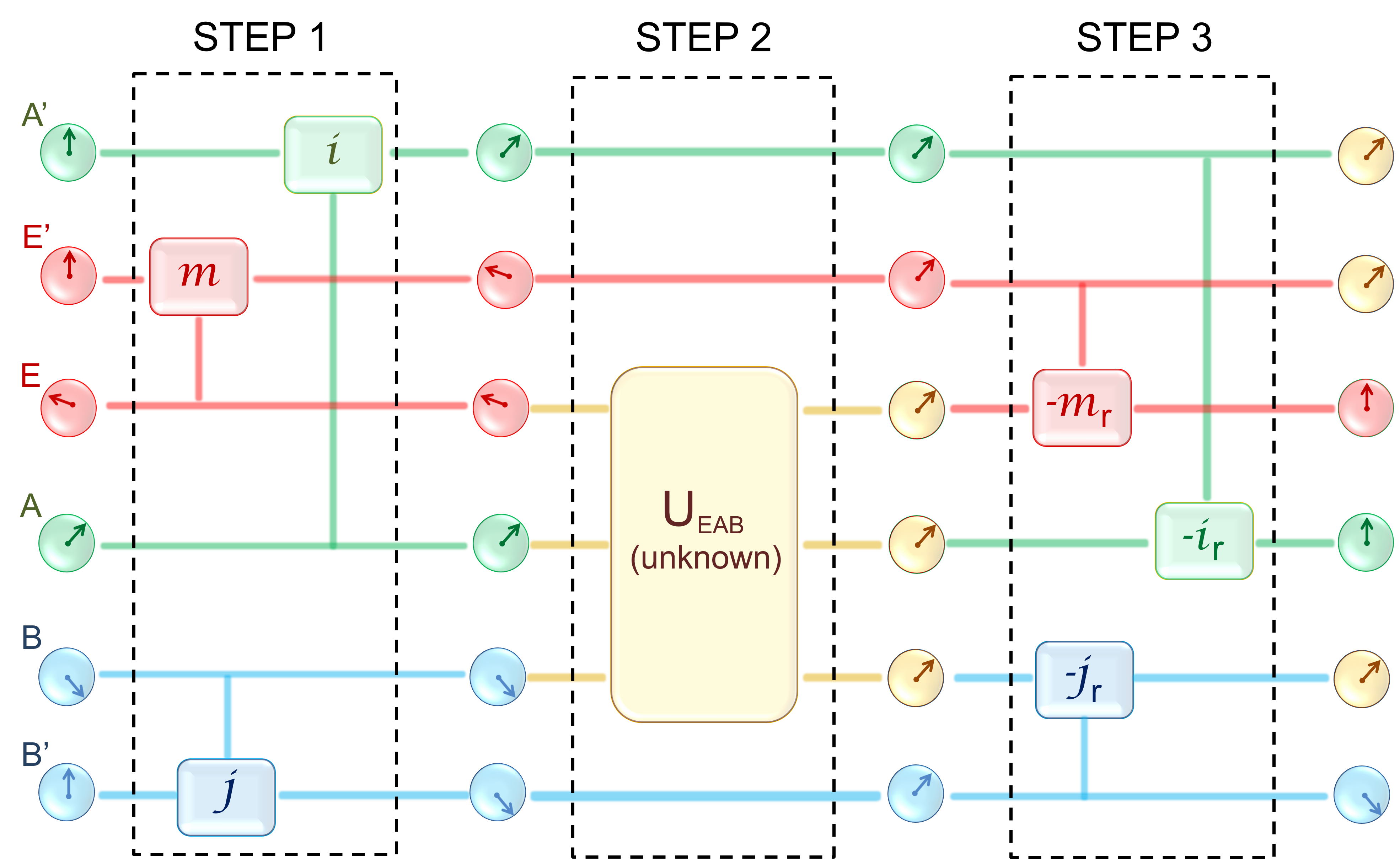
The degree of control of on given full information about , with respect to the reference bases , is then quantified by the difference between the OWI from to and the OWI from alone ( is ignored),
computed in the final state . The quantity, while giving different results from the OWI evaluated without information on , , inherits by construction the consistency and asymmetry properties. It is also explicitly computable for tripartite dynamics of classical and quantum systems, including Toffoli and bipartite controlled gates (Table 2). A quantifier of classical conditional causation as a special case is obtained by computing the conditional mutual information in the final state after it is projected into the reference bases. The extension to many-body processes of arbitrary size is straightforward. Given an -partite system evolving via the unitary , the OWI sent from a subsystem to a subsystem is
| (7) |
The chain rule of the conditional mutual information implies that the total OWI received from a subsystem is decomposable as the sum of conditional causations.
IV Conclusion
I have introduced a scheme to evaluate OWI (one-way information) generated via a quantum channel (Fig. 1). Then, I have built an information-theoretic measure of OWI, Eq. 5. The study paves the way for a resource theory of OWI gour , a mathematical framework studying the computational power of causal, one-way information flow costajin . OWI, rather than correlation, could be the key resource when different parts of a composite system play different roles, e.g. control control , metrology metrology , and learning learning . As OWI can be evaluated from correlation dynamics, one may build measures of genuine quantum and classical information flow, as it happens for correlation quantifiers modirev .
V Acknowledgements
I thank Chao Zhang for useful comments. The research presented in this article was supported by the R. Levi Montalcini Fellowship of the Italian Ministry of Research and Education, and the Laboratory Directed Research and Development program of Los Alamos National Laboratory under project number 20180702PRD1. Los Alamos National Laboratory is managed by Triad National Security, LLC, for the National Nuclear Security Administration of the U.S. Department of Energy under Contract No. 89233218CNA000001.
References
- (1) C. W. J. Granger, Investigating Causal Relations by Econometric Models and Cross-spectral Methods, Econometrica 37, 424 (1969).
- (2) J. Massey, Causality, Feedback And Directed Information, Proceedings of International Symposium on Information Theory and its Applications 30, (1990).
- (3) J. Pearl, Causality: Models, Reasoning, and Inference, Cambridge University Press (2000).
- (4) J. Peters, D. Janzing, and B. Schölkopf, Elements of Causal Inference, MIT Press (2017).
- (5) D. Rubin, Causal Inference Using Potential Outcomes, J. Amer. Statist. Assoc. 100, 322 (2005).
- (6) R. R. Tucci, An Information Theoretic Measure of Judea Pearl’s Identifiability and Causal Influence, arXiv:1307.5837.
- (7) R. G. James, N. Barnett, and J. P. Crutchfield, Information Flows? A Critique of Transfer Entropies, Phys. Rev. Lett. 116, 238701 (2016).
- (8) D. Janzing, D. Balduzzi, M. Grosse-Wentrup, and B. Schölkopf, Quantifying Causal Influences, The Annals of Statistics 41, 2324 (2013).
- (9) R. Horodecki, P. Horodecki, M. Horodecki, and K. Horodecki, Quantum Entanglement, Rev. Mod. Phys. 81, 865 (2009).
- (10) K. Modi, A. Brodutch, H. Cable, T. Paterek, and V. Vedral, The classical-quantum boundary for correlations: Discord and related measures, Rev. Mod. Phys. 84, 1655 (2012).
- (11) O. Oreshkov, F. Costa, and C. Brukner, Quantum correlations with no causal order, Nature Comm. 3, 1092 (2012).
- (12) G. Chiribella, G. M. D’Ariano, P. Perinotti, and B. Valiron, Quantum computations without definite causal structure, Phys. Rev. A 88, 022318 (2013).
- (13) M. S. Leifer and R. W. Spekkens, Towards a formulation of quantum theory as a causally neutral theory of Bayesian inference, Phys. Rev. A 88, 052130 (2013).
- (14) R. Chaves, C. Majenz, and D. Gross, Information-theoretic implications of quantum causal structures, Nature Comm. 6, 5766 (2015).
- (15) F. Costa and S. Shrapnel, Quantum causal modelling, New J. Phys. 18, 063032 (2016).
- (16) J.-M. A. Allen, J. Barrett, D. C. Horsman, C. M. Lee, and R. W. Spekkens, Quantum common causes and quantum causal models. Phys. Rev. X 7, 031021 (2017).
- (17) F. A. Pollock, C. Rodríguez-Rosario, T. Frauenheim, M. Paternostro, and K. Modi, Non-Markovian quantum processes: complete framework and efficient characterisation, Phys. Rev. A 97, 012127 (2018).
- (18) D. Horsman, C. Heunen, M. F. Pusey, J. Barrett, and R. W. Spekkens, Can a quantum state over time resemble a quantum state at a single time?, Proc. R. Soc. A 473, 20170395 (2017).
- (19) E. G. Cavalcanti, Classical Causal Models for Bell and Kochen-Specker Inequality Violations Require Fine-Tuning, Phys. Rev. X 8, 021018 (2018).
- (20) G. Chiribella and D. Ebler, Quantum speedup in the identification of cause-effect relations, Nature Comm. 10, 1472 (2019).
- (21) M. A. Nielsen and I. L. Chuang, Quantum Computation and Quantum Information, Cambridge University Press (2000).
- (22) J. von Neumann, Mathematical Foundations of Quantum Mechanics, Princeton University Press (1955).
- (23) A. Barenco, C. H. Bennett, R. Cleve, D. P. DiVincenzo, N. Margolus, P. Shor, T. Sleator, J. Smolin, and H. Weinfurter, Elementary gates for quantum computation, Phys. Rev. A 52, 3457 (1995).
- (24) E. G. Rieffel and W. H. Polak, Quantum Computing: A Gentle Introduction, MIT Press (2011).
- (25) P. Zanardi, C. Zalka, and L. Faoro, Entangling power of quantum evolutions, Phys. Rev. A 62, 030301(R) (2000).
- (26) M. Jiang, S. Luo, and S. Fu, Channel-state duality, Phys. Rev. A 87, 022310 (2013).
- (27) No correlations in both input and output states does not preclude interaction. A physical, continuous time implementation of a controlled gate from an uncorrelated input to an uncorrelated output may generate correlations at some time .
- (28) T. Cover and J. Thomas, Elements of Information Theory, Wiley (1991).
- (29) The letter is picked as the measure quantifies the strength of the causal link or, in other words, the degree of Control of a system on another.
- (30) J. Ma, B. Yadin, D. Girolami, V. Vedral, and M. Gu, Converting Coherence to Quantum Correlations, Phys. Rev. Lett. 116, 160407 (2016).
- (31) M. Piani, P. Horodecki, and R. Horodecki, No-Local-Broadcasting Theorem for Multipartite Quantum Correlations, Phys. Rev. Lett. 100, 090502 (2008).
- (32) T. Schreiber, Measuring Information Transfer, Phys. Rev. Lett. 85, 461 (2000).
- (33) J. Sun and E. M. Bollt, Causation Entropy Identifies Indirect Influences, Dominance of Neighbors and Anticipatory Couplings, Physica D 267, 49 (2014).
- (34) K. Fujii, Exchange gate on the qudit space and Fock space, J. Opt. B 5, S613 (2003).
- (35) E. Chitambar and G. Gour, Quantum resource theories, Rev. Mod. Phys. 91, 025001 (2019).
- (36) D. Jia, and F. Costa, Causal order as a resource for quantum communication, arXiv:1901.09159.
- (37) D. Dong and I. R. Petersen, Quantum control theory and applications: a survey, IET Cont. Th. App. 4, 2651 (2010).
- (38) V. Giovannetti, S. Lloyd, and L. Maccone, Advances in Quantum Metrology, Nature Phot. 5, 222 (2011).
- (39) P. Wittek. Quantum Machine Learning: What Quantum Computing Means to Data Mining, Academic Press (2014).