PixelHop: A Successive Subspace Learning (SSL) Method for Object Classification

Abstract

A new machine learning methodology, called successive subspace learning (SSL), is introduced in this work. SSL contains four key ingredients: 1) successive near-to-far neighborhood expansion; 2) unsupervised dimension reduction via subspace approximation; 3) supervised dimension reduction via label-assisted regression (LAG); and 4) feature concatenation and decision making. An image-based object classification method, called PixelHop, is proposed to illustrate the SSL design. It is shown by experimental results that the PixelHop method outperforms the classic CNN model of similar model complexity in three benchmarking datasets (MNIST, Fashion MNIST and CIFAR-10). Although SSL and deep learning (DL) have some high-level concept in common, they are fundamentally different in model formulation, the training process and training complexity. Extensive discussion on the comparison of SSL and DL is made to provide further insights into the potential of SSL.

Keywords Machine Learning  $\cdot$ Subspace Learning  $\cdot$ Computer Vision  $\cdot$ Pattern Recognition

1 Introduction

Subspace methods have been widely used in signal/image processing, pattern recognition, computer vision, etc. [1, 2, 3, 4, 5, 6]. They can have different names and emphasis in various contexts such as manifold learning [7, 8]. Generally speaking, one uses a subspace to denote the feature space of a certain object class, (e.g., the subspace of the dog object class) or the dominant feature space by dropping less important features (e.g., the subspace obtained via principal component analysis or PCA). The subspace representation offers a powerful tool for signal analysis, modeling and processing. Subspace learning is to find subspace models for concise data representation and accurate decision making based on training samples.

Most existing subspace methods are conducted in a single stage. We may ask whether there is an advantage to perform subspace learning in multiple stages. Research on generalizing from one-stage subspace learning to multi-stage subspace learning is rare. Two PCA stages are cascaded in the PCAnet [9], which provides an empirical solution to multi-stage subspace learning. Little research on this topic may be attributed to the fact that a straightforward cascade of linear multi-stage subspace methods, which can be expressed as the product of a sequence of matrices, is equivalent to a linear one-stage subspace method. The advantage of linear multi-stage subspace methods may not be obvious from this viewpoint.

Yet, multi-stage subspace learning may be worthwhile under the following two conditions. First, the input subspace is not fixed but growing from one stage to the other. For example, we can take the union of a pixel and its eight nearest neighbors to form an input space in the first stage. Afterward, we enlarge the neighborhood of the center pixel from $3\times 3$ to $5\times 5$ in the second stage. Clearly, the first input space is a proper subset of the second input space. By generalizing it to multiple stages, it gives rise to a “successive subspace growing" process. This process exists naturally in the convolutional neural network (CNN) architecture, where the response in a deeper layer has a larger receptive field. In our words, it corresponds to an input of a larger neighborhood. Instead of analyzing these embedded spaces independently, it is advantageous to find a representation of a larger neighborhood using those of its constituent neighborhoods of smaller sizes in computation and storage efficiency. Second, special attention should be paid to the cascade interface of two consecutive stages as elaborated below.

When two consecutive CNN layers are in cascade, a nonlinear activation unit is used to rectify the outputs of convolutional operations of the first layer before they are fed to the second layer. The importance of nonlinear activation to the CNN performance is empirically verified, yet little research is conducted on understanding its actual role. Along this line, it was pointed out in [10] that there exists a sign confusion problem when two CNN layers are in cascade. To address this problem, Kuo et al. proposed the Saak (subspace approximation via augmented kernels) transform [11] and the Saab (subspace approximation via adjusted bias) transform [12] as an alternative to nonlinear activation. Both Saak and Saab transforms are variants of PCA. They are carefully designed to avoid sign confusion.

One advantage of adopting Saak/Saab transforms rather than nonlinear activation is that the CNN system is easier to explain [12]. Specifically, Kuo et al. [12] proposed the use of multi-stage Saab transforms to determine parameters of convolutional layers and the use of multi-stage linear least-squares (LLS) regression to determine parameters of fully-connected (FC) layers. Since all parameters of CNNs are determined in a feedforward manner without any backpropagation (BP) in this design, it is named the “feedforward design". Yet, the feedforward design is drastically different from the BP-based design. Retrospectively, the work in [12] offered the first “successive subspace learning (SSL)" design example although the SSL term was not explicitly introduced therein. Although being inspired by the deep learning (DL) framework, SSL is fundamentally different in its model formulation, training process and training complexity. We will conduct an in-depth comparison between DL and SSL in Sec. 4.

SSL can be applied but not limited to parameters design of a CNN. In this work, we will examine the feedforward design as well as SSL from a higher ground. Our current study is a sequel of cumulative research efforts as presented in [10, 11, 12, 13]. Here, we introduce SSL formally and discuss its similarities and differences with DL. To illustrate the flexibility and generalizability of SSL, we present an SSL-based machine learning system for object classification. It is called the PixelHop method. The block diagram of the PixelHop system deviates from the standard CNN architecture completely since it is not a network any longer. The word “hop” is borrowed from graph theory. For a target node in a graph, its immediate neighboring nodes connected by an edge are called its one-hop neighbors. Its neighboring nodes connected to itself through $n$ consecutive edges via the shortest path are the $n$-hop neighbors. The PixelHop method begins with a very localized region; namely, a single pixel denoted by ${\bf p}$. It is called the $0$-hop input. We concatenate the attributes of a pixel, and attributes of its one-hop neighbors to form a one-hop neighborhood denoted by $\mathfrak{N}_{1}({\bf p})$. We can keep enlarging the input by including larger neighborhood regions. This idea applies to structured data (e.g., images) as well as unstructured data (e.g., 3D point cloud sets). An SSL-based 3D point cloud classification scheme, called the PointHop method, was proposed in [14].

If we implement the above idea in a straightforward manner, the dimension of neighborhood $\mathfrak{N}_{i}({\bf p})$, where $i=1,2,\cdots,I$ is the stage index, will grow very fast as $i$ becomes larger. To control the rapid dimension growth of $\mathfrak{N}_{i}({\bf p})$, we use the Saab transform to reduce its dimension. Since no label is used in the Saab transform, it is an unsupervised dimension reduction technique. To reduce the dimension of the Saab responses at each stage furthermore, we exploit the label of training samples to perform supervised dimension reduction, which is implemented by a label-assisted regression (LAG) unit. As a whole, the PixelHop method provides an extremely rich feature set by integrating attributes from near-to-far neighborhoods of selected spatial locations. Finally, we adopt an ensemble method to combine features and train a classifier, such as the support vector machine (SVM) [15] and the random forest (RF) [16], to provide the ultimate classification result. Extensive experiments are conducted on three datasets (namely, MNIST, Fashion MNIST and CIFAR-10 datasets) to evaluate the performance of the PixelHop method. It is shown by experimental results that the PixelHop method outperforms classical CNNs of similar model complexity in classification accuracy while demanding much lower training complexity.

Our current work has three major contributions. First, we introduce the SSL notion explicitly and make a thorough comparison between SSL and DL. Second, the LAG unit using soft pseudo labels as presented in Sec. 2.3 is novel. Third, we use the PixelHop method as an illustrative example for SSL, and conduct extensive experiments to demonstrate its performance.

The rest of this paper is organized as follows. The PixelHop method is presented in Sec. 2. Experimental results of the PixelHop method are given in Sec. 3. Comparison between DL and SSL is discussed in Sec. 4. Finally, concluding remarks are drawn and future research topics are pointed out in Sec. 5.

2 PixelHop Method

We present the PixelHop method to illustrate the SSL methodology for image-based object classification in this section. First, we give an overview of the whole system in Sec. 2.1. Then, we study the properties of Saab filters that reside in each PixelHop unit in Sec. 2.2. Finally, we examine the label-assisted regression (LAG) unit of the PixelHop system in Sec. 2.3.

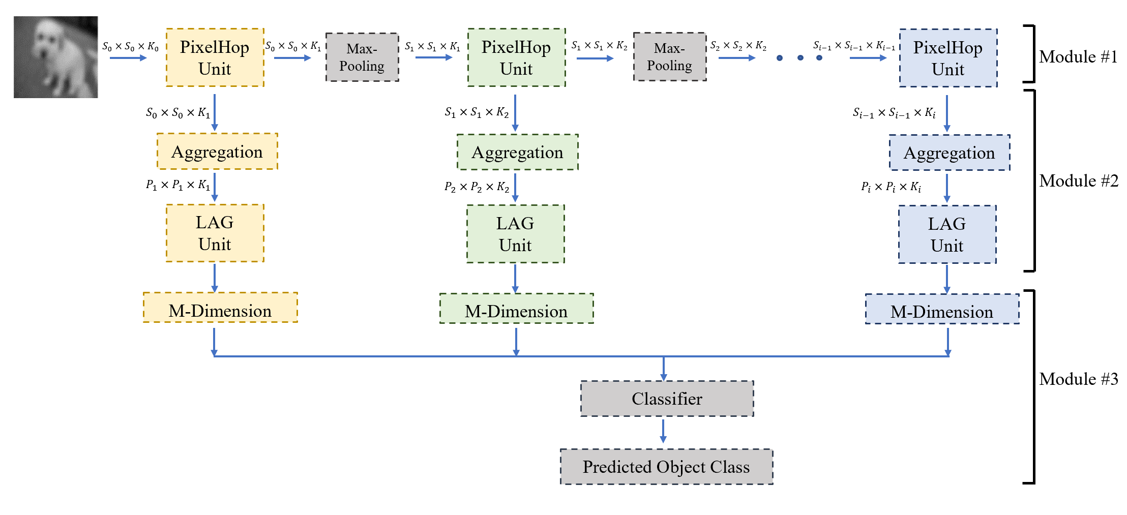
Figure 1: The block diagram of the PixelHop method.

2.1 System Overview

The block diagram of the PixelHop method is given in Fig. 1. Its input can be graylevel or color images. They are fed into a sequence of $I$ PixelHop units in cascade to obtain the attributes of the $i$th PixelHop unit, $i=1,2,\cdots,I$, as shown in module #1. The attributes in spatial locations of each PixelHop unit are aggregated in multiple forms and, then, fed into the LAG unit for further dimension reduction to generate $M$ attributes per unit as shown in module #2. Finally, these attributes are concatenated to form the ultimate feature vector of dimension $M\times I$ for image classification as shown in module #3. The function of each module is stated below.

• Module #1: A sequence of PixelHop units in cascade
  

  The purpose of this module is to compute attributes of near-to-far neighborhoods of selected pixels through $I$ PixelHop units. The block diagram of a PixelHop unit is shown in Fig. 2. The $i$th PointHop unit, $i=1,\cdots,I$, concatenates attributes of the $(i-1)$th neighborhood, whose dimension is denoted by $K_{(i-1)}$, of a target pixel and its $N_{i}$ neighboring pixels to form a neighborhood union. Through this process, the dimension of the enlarged neighborhood is equal to $K_{(i-1)}\times(N_{i}+1)$. Without loss of generality, we set $N_{i}=8$ for all $i$ in our implementation. If we do not take any further action, the attribute dimension will be $K_{0}9^{i}$ at the $i$th unit. It is critical to apply a dimension reduction technique so as to control the rapidly growing dimension. This is achieved by a subspace approximation technique; namely, the Saab transform, as illustrated in Fig. 3.

  Each PixelHop unit yields a neighborhood representation corresponding to its stage index and input neighborhood size. At the $i$th PixelHop unit, we see that the spectral dimension is reduced from $9K_{i-1}$ to $K_{i}$ after the Saab transform while the spatial dimension remains the same. Since the neighborhoods of two adjacent pixels are overlapping with each other at each PixelHop unit, there exists spatial redundancy in the attribute representation. For this reason, we insert the standard $(2\times 2)$-to-$(1\times 1)$ maximum pooling unit between two consecutive PixelHop units as shown in Fig. 1. After the pooling, the spatial resolution is reduced from $S_{(i-1)}\times S_{(i-1)}$ to $S_{i}\times S_{i}$.

  

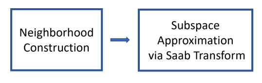
  Figure 2: The block diagram of a PixelHop unit in the PixelHop system.

  

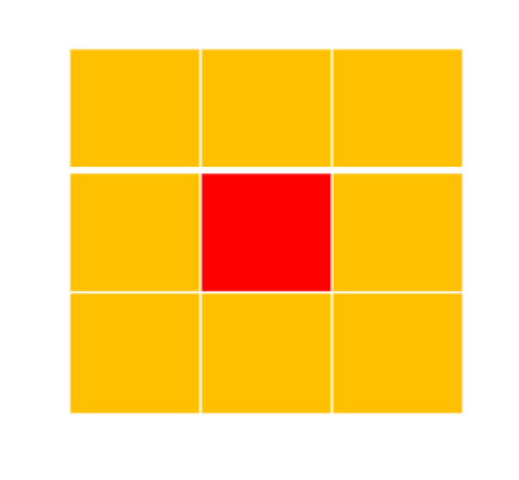
  (a)

  

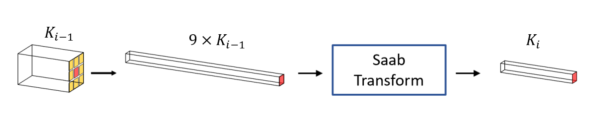
  (b)

  Figure 3: The block diagram of a PixelHop unit: (a) neighborhood construction by taking the union of a center pixel and its eight nearest neighborhood pixels and (b) the use of the Saab transform to reduce the dimension from $9K_{(i-1)}$ to $K_{i}$.

• Module #2: Aggregation and supervised dimension reduction via the label-assisted regression (LAG) unit
  

  The output from the $i$th PixelHop unit has a dimension of $S_{(i-1)}\times S_{(i-1)}\times K_{i}$ as illustrated in Fig. 4. The maximum pooling scheme is used to reduce the spatial dimension before the output is fed into the next PixelHop unit as described in module #1. To extract a diversified set of features at the $i$th stage, we consider multiple aggregation schemes such as taking the maximum, the minimum, and the mean values of responses in small nonoverlapping regions. The spatial size of features after aggregation is denoted as $P_{i}\times P_{i}$, where $P_{i}$ is a hyper-parameter to choose. We will explain the relationship between $P_{i}$ and $S_{i}$ in Sec. 3. Afterward, we reduce the feature dimension based on supervised learning. For a given neighborhood size, we expect attributes of different object classes to follow different distributions. For example, a cat image has fur texture while a car image does not. This property can be exploited to allow us to find a more concise representation, which will be elaborated in Sec. 2.3. In Fig. 1, we use $M$ to denote the dimension of the feature vector at each PixelHop unit.

  

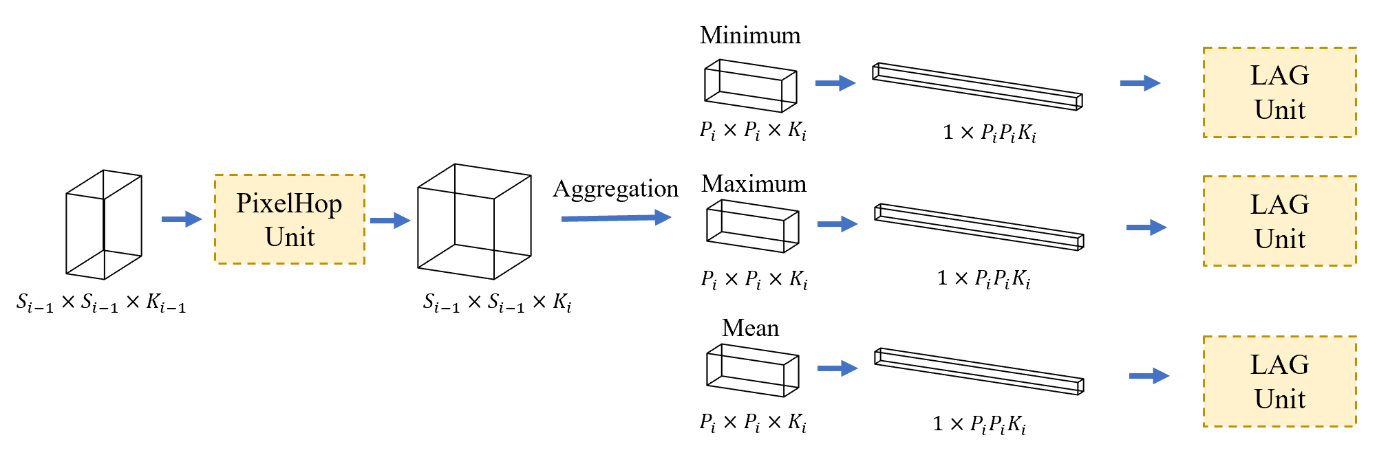
  Figure 4: Illustration of the aggregation unit in module #2.

• Module #3: Feature concatenation across all PixelHop units and Classification
  We concatenate $M$ features from $I$ PixelHop units to get a total of $M\times I$ features in module #3. Afterward, we train a multi-class classifier using these features by following the standard pattern recognition procedure. In the experiment, we use the SVM classifier with its kernel being the radial basis function (RBF).

2.2 Properties of Saab Filters

The Saab transform decomposes a signal space into two subspaces - the DC (direct current) subspace and the AC (alternating current) subspace. It uses the DC filter, which is a normalized constant-element vector, to represent the DC subspace. It applies PCA to the AC subspace to derive the AC filters. We will examine two issues below: 1) the relationship between the number of AC filters and the subspace approximation capability, and 2) the fast convergence behavior of AC filters.

Number of AC filters We show the relationship between the energy preservation ratio and the number of Saab AC filters in Fig. 5. We see that leading AC filters can capture a large amount of energy while the capability drops rapidly as the index becomes larger. We plot four energy thresholds: 95% (yellow), 96% (red), 97% (blue), 98% (green) and 99% (purple) in Fig. 5. This suggests that we may use a higher energy ratio in the beginning PixelHop units and a lower energy ratio in the latter PixelHop units if we would like to balance the classification performance and the complexity.

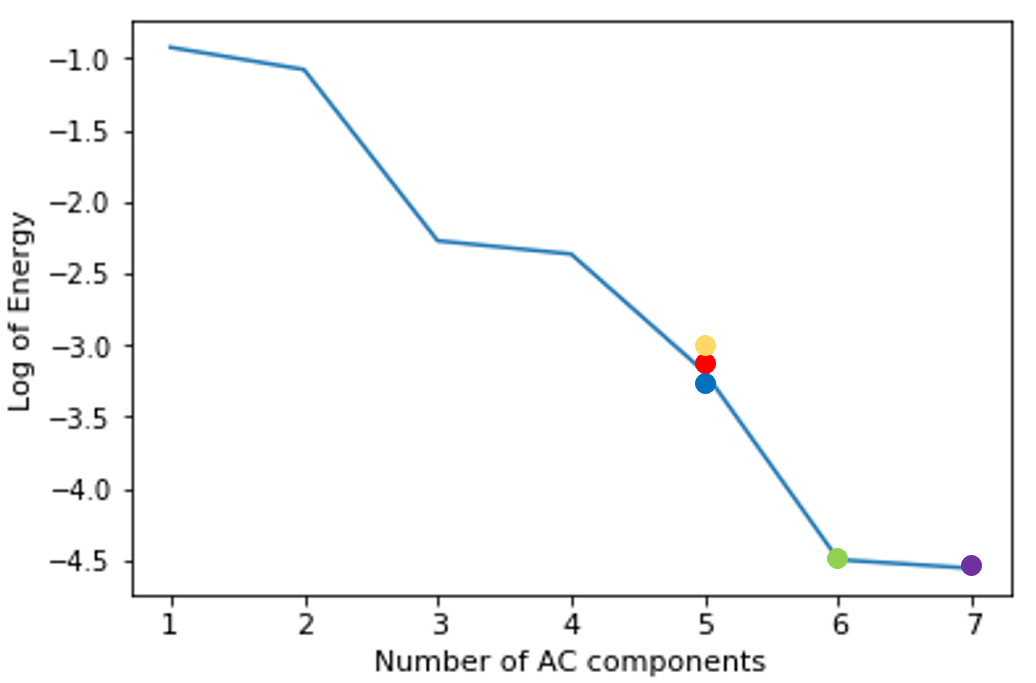
(a) PixelHop Unit1

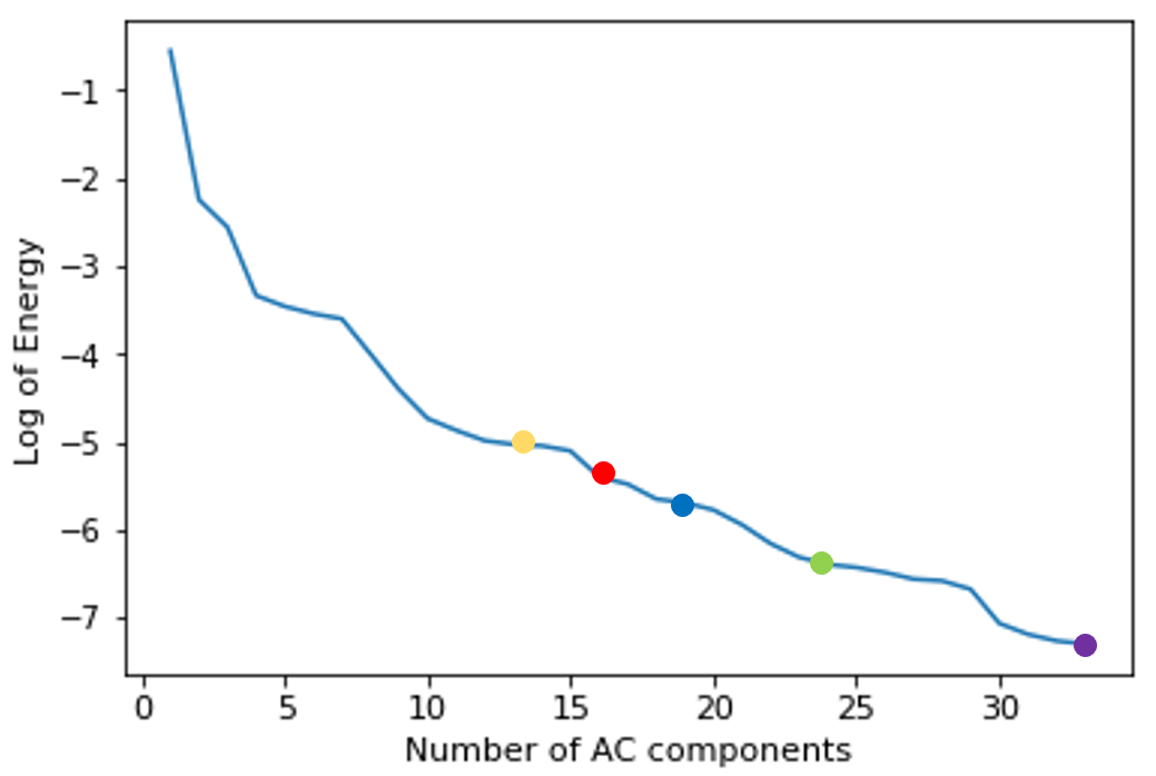
(b) PixelHop Unit2

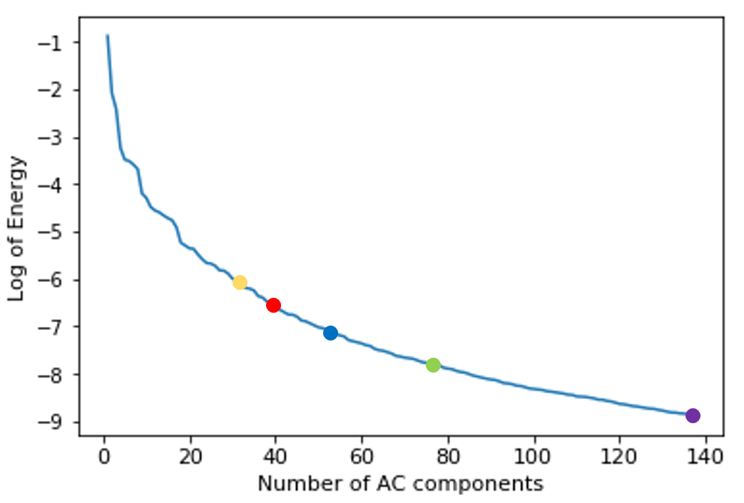
(c) PixelHop Unit3

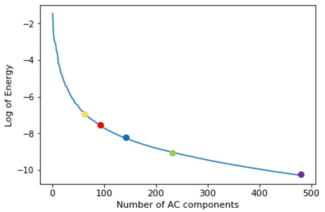
(d) PixelHop Unit4

Figure 5: The log energy plot as a function of the number of AC filters tested on the luminance (Y) channel of color images from CIFAR-10 dataset, where the yellow, red, blue, green and purple dots indicate the cumulative energy ratio of 95%, 96%, 97%, 98% and 99%, respectively.

Fast Convergence. Subspace approximation using the Saab transform is an unsupervised learning process. The unsupervised learning pipeline in module # of the PixelHop system actually does not demand a large number of data samples. We conduct experiments on the CIFAR-10 dataset as an example to support this claim. This system contains four PixelHop units, where the number of AC filters is chosen by setting the energy preservation ratio to $95\%$. The Saab filters are derived from the covariance matrix of DC-removed spatial-spectral cuboids. If the covariance matrix converges quickly, the Saab filters should converge fast as well. To check the convergence of the covariance matrix, we compute the Frobenius norm of the difference of two covariance matrices using $K_{t}$ and $K_{(t+1)}$ cuboid samples. We plot the dimension-normalized Frobenius norm difference, denoted by $\Delta_{(t+1)}$, as a function of $K_{(t+1)}$ in Fig. 6. The curve is obtained as the average of five runs. We see that the Frobenius norm difference converges to zero very rapidly, indicating a fast-converging covariance matrix. Furthermore, we compute the cosine similarity between the converged Saab filters (using all 50K training images of the dataset) as well as Saab filters obtained using a certain number of images. The results are shown in Fig. 7. We see that AC filters converge to the final one with about 1K training images in the first two PixelHop units and about 2.5K training images in the last two PixelHop units.

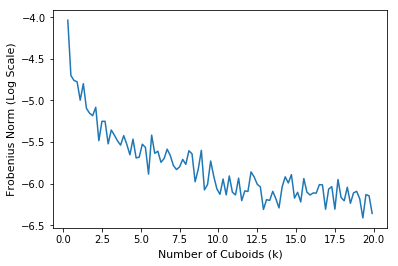
(a) PixelHop Unit1

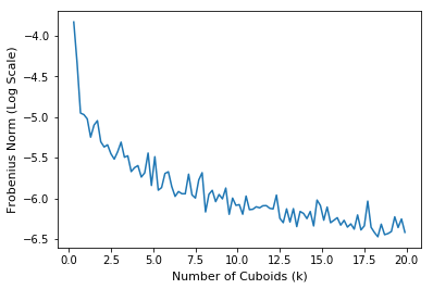
(b) PixelHop Unit2

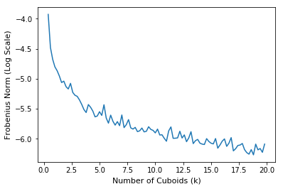
(c) PixelHop Unit3

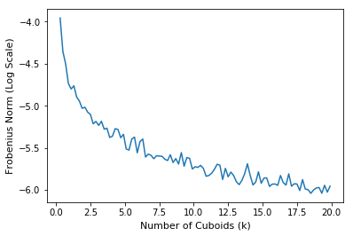
(d) PixelHop Unit4

Figure 6: The Frobenius norm of the difference of two covariance matrices, $\Delta_{(t+1)}$, using $K_{t}$ and $K_{(t+1)}$ sample patches is plotted as a function of $K_{(t+1)}$.

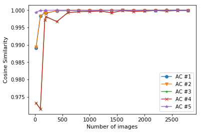
(a) PixelHop Unit1

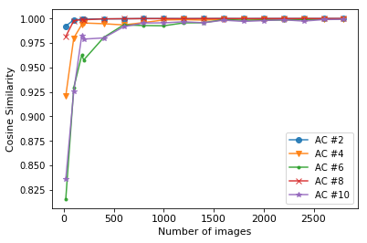
(b) PixelHop Unit2

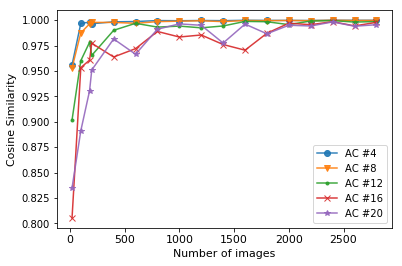
(c) PixelHop Unit3

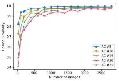
(d) PixelHop Unit4

Figure 7: The cosine similarity between the AC filters obtained using all training images and those obtained using a certain number of images is plotted as a function of the number of images of the latter. Five representative AC filters at each PixelHop unit are selected for the illustration purpose.

2.3 Label-Assisted Regression (LAG)

Our design of the Label-Assisted reGression (LAG) unit is motivated by two observations. First, each PixelHop unit offers a representation of a neighborhood of a certain size centered at a target pixel. The size varies from small to large ones through successive neighborhood expansion and subspace approximation. The representations are called attributes. We need to integrate the local-to-global attributes across multiple PixelHop units at multiple selected pixels to solve the image classification problem. One straightforward integration is to concatenate all attributes to form a long feature vector. Yet, the dimension of concatenated attributes is too high to be effective. We need another way to lower the dimension of the concatenated attributes. Second, CNNs use data labels effectively through BP. It is desired to find a way to use data labels in SSL. The attributes of the same object class are expected to reside in a smaller subspace in high-dimensional attribute space. We attempt to search for the subspace formed by samples of the same class for dimension reduction. This procedure demands a supervised dimension reduction technique.

Although being presented in different form, a similar idea was investigated in [12]. To give an interpretation to the first FC layer of the LeNet-5, Kuo et al. [12] proposed to partition samples of each digit class into 12 clusters to generate 12 pseudo-classes to account for intra-class variabilities. By mimicking the dimension of the first FC layer of the LeNet-5, we have 120 clusters (i.e., 12 clusters per digit for 10 digits) in total. Since each training sample belongs to one of 120 clusters, we assign it to a one-hot vector in a space of dimension 120. Then, we can set up a least-squared regression (LSR) system containing 120 affine equations that map samples in the input feature space to the output space that is formed by 120 one-hot vectors. The one-hot vector is used to indicate a cluster with a hard label. In this work, we adopt soft-labeled output vectors in setting up the LSR problem. The learning task is to use the training samples to determine the elements in the regression matrix. Then, we apply the learned regression matrix to testing samples for dimension reduction.

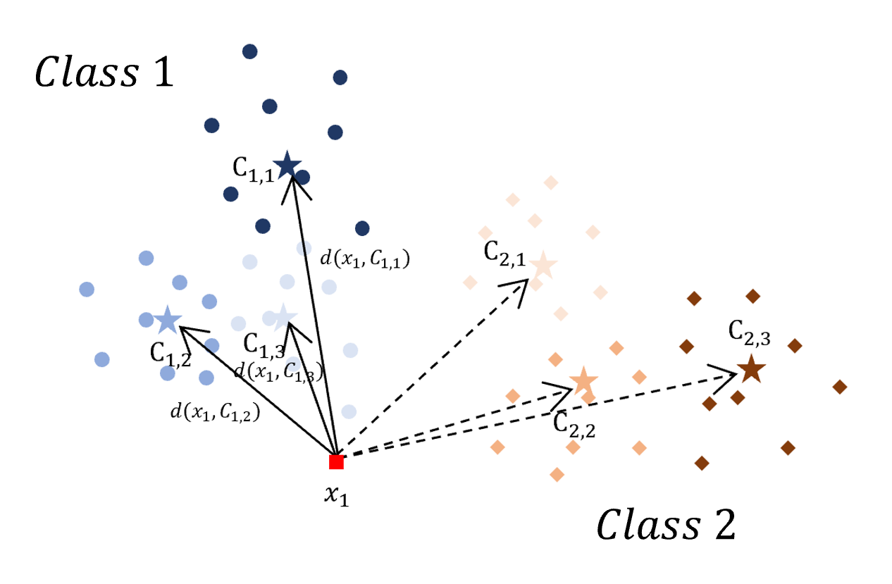
Figure 8: Illustration of the relationship between a feature point and centroids of different classes in the LAG unit.

By following the notation in Fig. 4, after spatial aggregation, the $i$th PixelHop unit yields a vector of dimension $1\times P_{i}P_{i}K_{i}$, where $P_{i}\times P_{i}$ denotes the number of selected pixels and $K_{i}$ denotes the attribute number. As illustrated in Fig. 8, we study the distribution of these concatenated attribute vectors based on their labels through the following steps:

1. We cluster samples of the same class to create object-oriented subspaces and find the centroid of each subspace.

2. Instead of adopting a hard association between samples and centroids, we adopt a soft association. As a result, the target output vector is changed from the one-hot vector to a probability vector.

3. We set up and solve a linear LSR problem using the probability vectors.

The regression matrix obtained in the last step is the label-assisted regressor.

For Step #1, we adopt the k-means clustering algorithm. It applies to samples of the same class only. We partition samples of each class into $L$ clusters Suppose that there are $J$ object classes, denoted by $O_{j}$, $j=1,\cdots,J$ and the dimension of the concatenated attribute vectors is $n$. For Step #2, we denote the vector of concatenated attributes of class $O_{j}$ by ${\bf x}_{j}=(x_{j,1},x_{j,2},\cdots,x_{j,n})^{T}\in R^{n}$. Also, we denote centroids of $L$ clusters by ${\bf c}_{j,1}$, ${\bf c}_{j,2}$, $\cdots$, ${\bf c}_{j,L}$. Then, we define the probability vector of sample ${\bf x}_{j}$ belonging to centroid ${\bf c}_{j^{\prime},l}$ as

$$\mbox{Prob}({\bf x}_{j},{\bf c}_{j^{\prime},l})=0\quad\mbox{if}j\neq j^{\prime},$$ (1)

and

$$\mbox{Prob}({\bf x}_{j},{\bf c}_{j,l})=\frac{\exp(-\alpha d({\bf x}_{j},{\bf c}_{j,l}))}{\sum_{l=1}^{L}\exp(-\alpha d({\bf x}_{j},{\bf c}_{j,l}))},$$ (2)

where $d({\bf x},{\bf y})$ is the Euclidean distrance between vectors ${\bf x}$ and ${\bf y}$ and $\alpha$ is a parameter to determine the relationship between the Euclidean distance and the likelihood for a sample belonging to a cluster. The larger $\alpha$, the probability decays faster with the distance. The short the Euclidean distance, the larger the likelihood. Finally, we can define the probability of sample ${\bf x}$ belonging to a subspace spanned by centroids of class $j$ as

$${\bf p}_{j}({\bf x}_{j^{\prime}})={\bf 0},\quad\mbox{if}j\neq j^{\prime},$$ (3)

where ${\bf 0}$ is the zero vector of dimension $L$, and

$${\bf p}_{j}({\bf x}_{j})=(\mbox{Prob}({\bf x}_{j},{\bf c}_{j,1}),\cdots\mbox{Prob}({\bf x}_{j},{\bf c}_{j,l}),\cdots\mbox{Prob}({\bf x}_{j},{\bf c}_{j,L}))^{T}.$$ (4)

Finally, we can set up a set of linear LSR equations to relate the input attribute vector and the output probability vector as

$$\left[\begin{array}[]{ccccc}a_{11}&a_{12}&\cdots&a_{1n}&w_{1}\\ a_{21}&a_{22}&\cdots&a_{2n}&w_{2}\\ \vdots&\vdots&\ddots&\vdots&\vdots\\ a_{M1}&a_{M2}&\cdots&a_{Mn}&w_{M}\end{array}\right]\left[\begin{array}[]{c}x_{1}\\ x_{2}\\ \vdots\\ x_{n}\\ 1\end{array}\right]=\left[\begin{array}[]{c}{\bf p}_{1}({\bf x})\\ \vdots\\ {\bf p}_{j}({\bf x})\\ \vdots\\ {\bf p}_{J}({\bf x})\\ \end{array}\right],$$ (5)

where $M=J\times L$ is the total number of centroids, parameters $w_{1}$, $w_{2}$, $\cdots$, $w_{M}$ are the bias terms and ${\bf p}_{j}({\bf x})$ is defined in Eq. (4). It is the probability vector of dimension $L$, which indicates the likelihood for input ${\bf x}$ to belong to the subspace spanned by the centroids of class $j$. Since ${\bf x}$ can belong to one class only, we have zero probability vectors with respect to $J-1$ classes.

3 Experimental Results

We organize experimental results in this section as follows. First, we discuss the experimental setup in Sec. 3.1. Second, we conduct the ablation study and study the effects of different parameters on the Fashion MNIST dataset in Sec. 3.2. Third, we perform error analysis, compare the performance of color image classification using different color spaces and show the scalability of the PixelHop method in Sec. 3.3. Finally, we conduct performance benchmarking between the PixelHop method and the LeNet-5 network [17], which is a classical CNN architecture of model complexity similar to the PixelHop method in terms of classification accuracy and training complexity in Sec. 3.4.

3.1 Experiment Setup

We test the classification performance of the PixelHop method on three popular datasets: MNIST [17], Fashion MNIST [18] and CIFAR-10 [19]. The MNIST dataset contains gray-scale images of handwritten digits (from $0$ to $9$). It has 60,000 training images and 10,000 testing images. The original image size is $28\times 28$ and zero-padding is used to enlarge the image size to $32\times 32$. The Fashion MNIST dataset contains gray-scale fashion images. Its image size and numbers of training and testing images are the same as those of the MNIST dataset. The CIFAR-10 dataset has 10 object classes of color images and the image size is $32\times 32$. It has 50,000 training images and 10,000 testing images.

The following parameters are used in the default setting, called PixelHop, in our experiments.

1. Four PixelHop units are cascaded in module #1. To decide the number of Saab AC filters in the unsupervised dimension reduction procedure, we set the total energy ratio preserved by AC filters to 97% for MNIST and Fashion MNIST and 98% for CIFAR-10.

2. To aggregate attributes spatially in module #2, we average responses of nonoverlapping patches of sizes $4\times 4$, $4\times 4$, $2\times 2$ and $2\times 2$ in the first, second, third and fourth PixelHop units, respectively, to reduce the spatial dimension of attribute vectors. Mathematically, we have

   $$P_{1}=0.25S_{0},\quad P_{2}=0.25S_{1},\quad P_{3}=0.5S_{2},\quad P_{4}=0.5S_{3}.$$ (6)

   As a result, the first to the fourth PixelHop units have outputs of dimension $8\times 8\times K_{1}$, $4\times 4\times K_{2}$, $4\times 4\times K_{3}$, and $2\times 2\times K_{4}$, respectively. Then, we feed all of them to the supervised dimension reduction unit.

3. We set $\alpha=10$ and the number of clusters for each object class to $L=5$ in the LAG unit of module #2. Since there are $J=10$ object classes in all three datasets of concern, the dimension is reduced to $J\times L=50$.

4. We use the multi-class SVM classifier with the Radial Basis Function (RBF) as the kernel in module #3. Before training the SVM classifier, we normalize each feature dimension to be a zero mean random variable with the unit variance.

Although the hyper parameters given above are chosen empirically, the final performance of the PixelHop system is relatively stable if their values are in the ballpark.

3.2 Ablation Study

Table 1: Ablation study for Fashion MNIST, where the fourth and the eighth rows are the settings adopted by PixelHop and PixelHop⁺, respectively.

Feature Used		DR		Aggregation				Classifier		Test ACC (%)
ALL	Last Unit	LAG	PCA	Mean	Min	Max	Skip	SVM	RF
	✓	✓		✓				✓		89.88
	✓		✓	✓				✓		89.11
✓		✓		✓					✓	89.31
✓		✓		✓				✓		91.30
✓		✓			✓			✓		91.16
✓		✓				✓		✓		90.83
✓		✓					✓	✓		91.14
✓		✓		✓	✓	✓		✓		91.68

We use the Fashion MNIST dataset as an example of the ablation study. We show the test averaged classification accuracy (ACC) results for the Fashion MNIST dataset under different settings in Table 1. We can reach a classification accuracy of 91.30% with the default setting (see the fourth row). It is obtained by concatenating image representations from all four PixelHop units, using mean-pooling to reduce the spatial dimension of attribute vectors, label-assisted regression (LAG) and the SVM classifier. Furthermore, we can boost the classification accuracy by adopting three pooling schemes (i.e. max-, mean- and min-pooling) together (see the eighth row). This is called PixelHop⁺.

We compare the classification performance using the output of an individual PixelHop unit, PixelHop and PixelHop⁺ in Table 2. We see from the table clear advantages of aggregating features across all PixelHop units.

Table 2: Comparison of the classification accuracy (%) using features from an individual PixelHop unit, PixelHop and PixelHop⁺ for Fashion MNIST.

Dataset	HOP-1	HOP-2	HOP-3	HOP-4	PixelHop	PixelHop+
MINST	97.00	98.35	98.45	98.71	98.90	99.09
Fashion MINST	87.38	89.35	89.96	89.88	91.30	91.68
CIFAR-10	52.27	67.86	69.08	67.91	71.37	72.66

Number of Saab AC filters. We study the relationship between the classification performance and the energy preservation ratio of the Saab AC filters in Fig. 9, where the $x$-axis indicates the cumulative energy ratio preserved by AC filters. Although preserving more AC energy can improve the classification performance, the rate of improvement is slow. On the other hand, we need to pay a price of adding more AC filters. The corresponding AC filter numbers at each PixelHop unit at each energy threshold value are listed in Fig. 9 to illustrate the performance-complexity tradeoff.

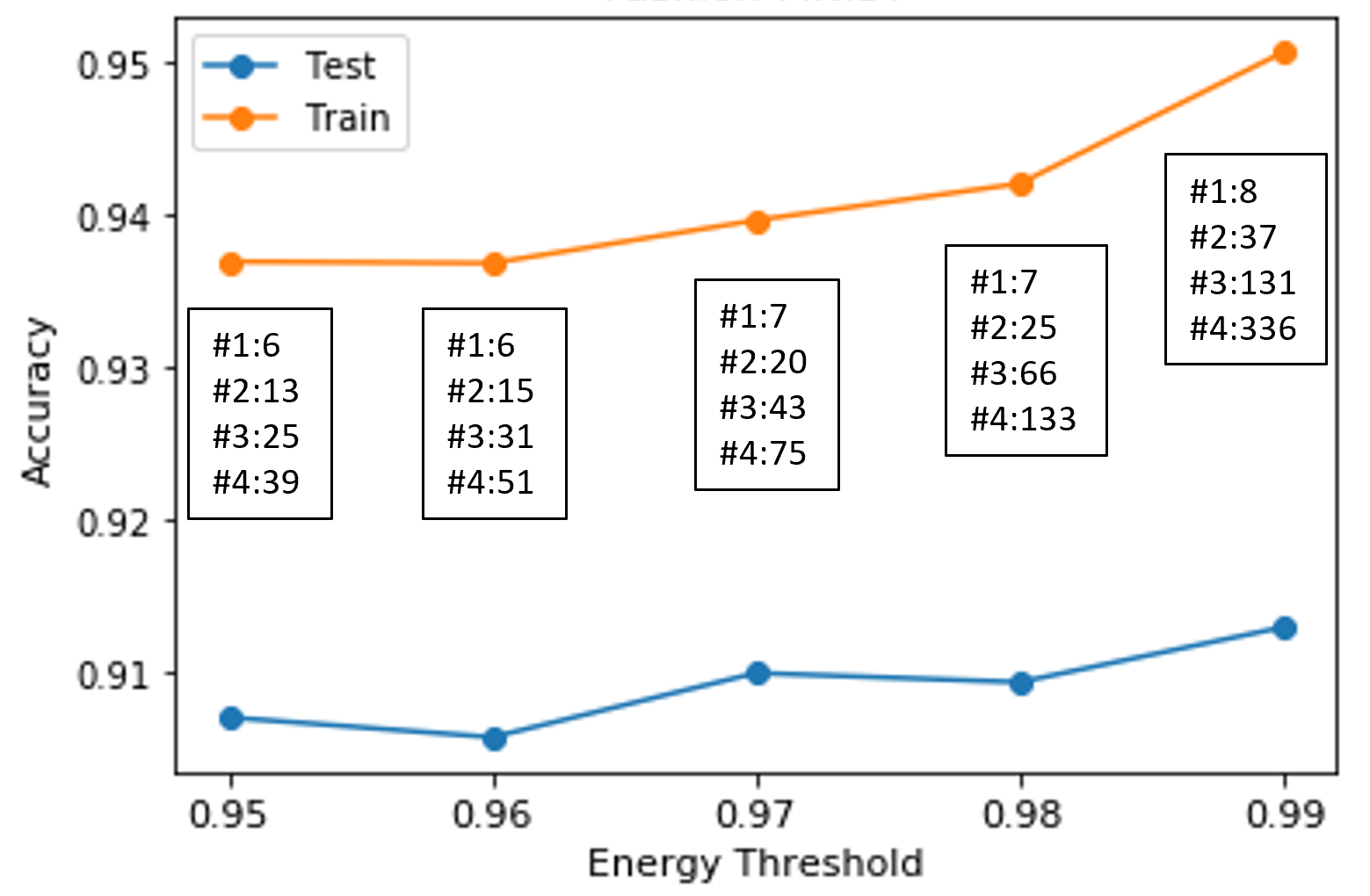
Figure 9: The classification accuracy as a function of the total energy preserved by AC filters tested on Fashion MNIST, where the corresponding AC filter numbers at each PixelHop unit are also listed to illustrate the performance-complexity tradeoff.

Table 3: The confusion matrix for the MNIST dataset, where the first row shows the predicted object labels and the first column shows the true object labels.

	0	1	2	3	4	5	6	7	8	9
0	0.996	0.000	0.000	0.000	0.001	0.000	0.001	0.001	0.001	0.000
1	0.000	0.997	0.001	0.000	0.000	0.001	0.001	0.000	0.000	0.000
2	0.000	0.002	0.992	0.000	0.000	0.000	0.000	0.003	0.002	0.001
3	0.000	0.000	0.002	0.995	0.000	0.000	0.000	0.001	0.002	0.000
4	0.000	0.000	0.003	0.000	0.991	0.000	0.001	0.000	0.001	0.004
5	0.001	0.000	0.000	0.000	0.000	0.998	0.001	0.000	0.000	0.000
6	0.003	0.002	0.000	0.000	0.001	0.004	0.987	0.000	0.002	0.000
7	0.000	0.002	0.008	0.001	0.000	0.000	0.000	0.986	0.001	0.002
8	0.003	0.000	0.004	0.001	0.001	0.000	0.000	0.002	0.986	0.003
9	0.001	0.002	0.003	0.002	0.006	0.001	0.000	0.003	0.002	0.980

Table 4: The confusion matrix for the Fashion MNIST dataset, where the first row shows the predicted object labels and the first column shows the true object labels.

	T-shirt/top	Trouser	Pullover	Dress	Coat	Sandal	Shirt	Sneaker	Bag	Ankle boot
T-shirt/top	0.883	0.000	0.015	0.016	0.005	0.000	0.072	0.000	0.009	0.000
Trouser	0.001	0.980	0.000	0.013	0.002	0.000	0.002	0.000	0.002	0.000
Pullover	0.015	0.001	0.877	0.009	0.053	0.000	0.044	0.000	0.001	0.000
Dress	0.017	0.006	0.010	0.919	0.023	0.000	0.022	0.000	0.003	0.000
Coat	0.000	0.001	0.056	0.027	0.866	0.000	0.050	0.000	0.000	0.000
Sandal	0.000	0.000	0.000	0.000	0.000	0.979	0.000	0.016	0.000	0.005
Shirt	0.110	0.000	0.048	0.021	0.072	0.000	0.742	0.000	0.007	0.000
Sneaker	0.000	0.000	0.000	0.000	0.000	0.010	0.000	0.971	0.000	0.019
Bag	0.003	0.001	0.003	0.002	0.002	0.001	0.001	0.004	0.983	0.000
Ankle boot	0.000	0.000	0.000	0.000	0.000	0.005	0.001	0.026	0.000	0.968

Table 5: The confusion matrix for the CIFAR-10 dataset, where the first row shows the predicted object labels and the first column shows the true object labels.

	airplane	automobile	bird	cat	deer	dog	frog	horse	ship	truck
airplane	0.783	0.023	0.034	0.017	0.014	0.008	0.012	0.009	0.067	0.033
automobile	0.029	0.827	0.010	0.011	0.001	0.005	0.007	0.002	0.023	0.085
bird	0.062	0.006	0.618	0.064	0.082	0.071	0.061	0.016	0.009	0.011
cat	0.023	0.016	0.071	0.549	0.061	0.174	0.056	0.030	0.008	0.012
deer	0.032	0.003	0.070	0.062	0.695	0.031	0.043	0.051	0.011	0.002
dog	0.011	0.006	0.059	0.196	0.049	0.601	0.026	0.037	0.009	0.006
frog	0.007	0.005	0.049	0.059	0.025	0.027	0.822	0.002	0.003	0.001
horse	0.023	0.008	0.033	0.048	0.052	0.070	0.007	0.755	0.001	0.003
ship	0.063	0.042	0.011	0.017	0.002	0.006	0.003	0.006	0.821	0.029
truck	0.036	0.080	0.010	0.016	0.008	0.009	0.005	0.013	0.028	0.795

3.3 Error Analysis, Color Spaces and Scalability

Error Analysis. We provide confusion matrices for MNIST, fashion MNIST and CIFAR-10 in Table 3, Table 4 and Table 5, respectively. Furthermore, we show some error cases in Fig. 10 and have the following observations.

• For the MNIST dataset, the misclassified samples are truly challenging. To handle these hard samples, we may need to turn to a rule-based method. For example, humans often write “4" in two strokes and “9" in one stroke. If we can identify the troke number from a static image, we can use the information to make a better prediction.

• For the Fashion MNIST dataset, we see that the “shirt" class is the most challenging one. As shown in Fig. 10, the shirt class is a general class that overlaps with the “top", the “pullover" and the “coat" classes. This is the main source of erroneous classifications.

• For the CIFAR-10 dataset, the “dog" class can be confused with the “cat" class. As compared with other object classes, the “dog" and the “cat" classes share more visual similarities. On one hand, it may demand more distinctive features to differentiate them. On the other hand, the error is caused by the poor image resolution. The “Ship" and the “airplane" classes form another confusing pair. The background is quite similar in these two object classes, i.e. containing the blue sky and the blue ocean. It is a challenging task to recognize small objects in poor resolution images.

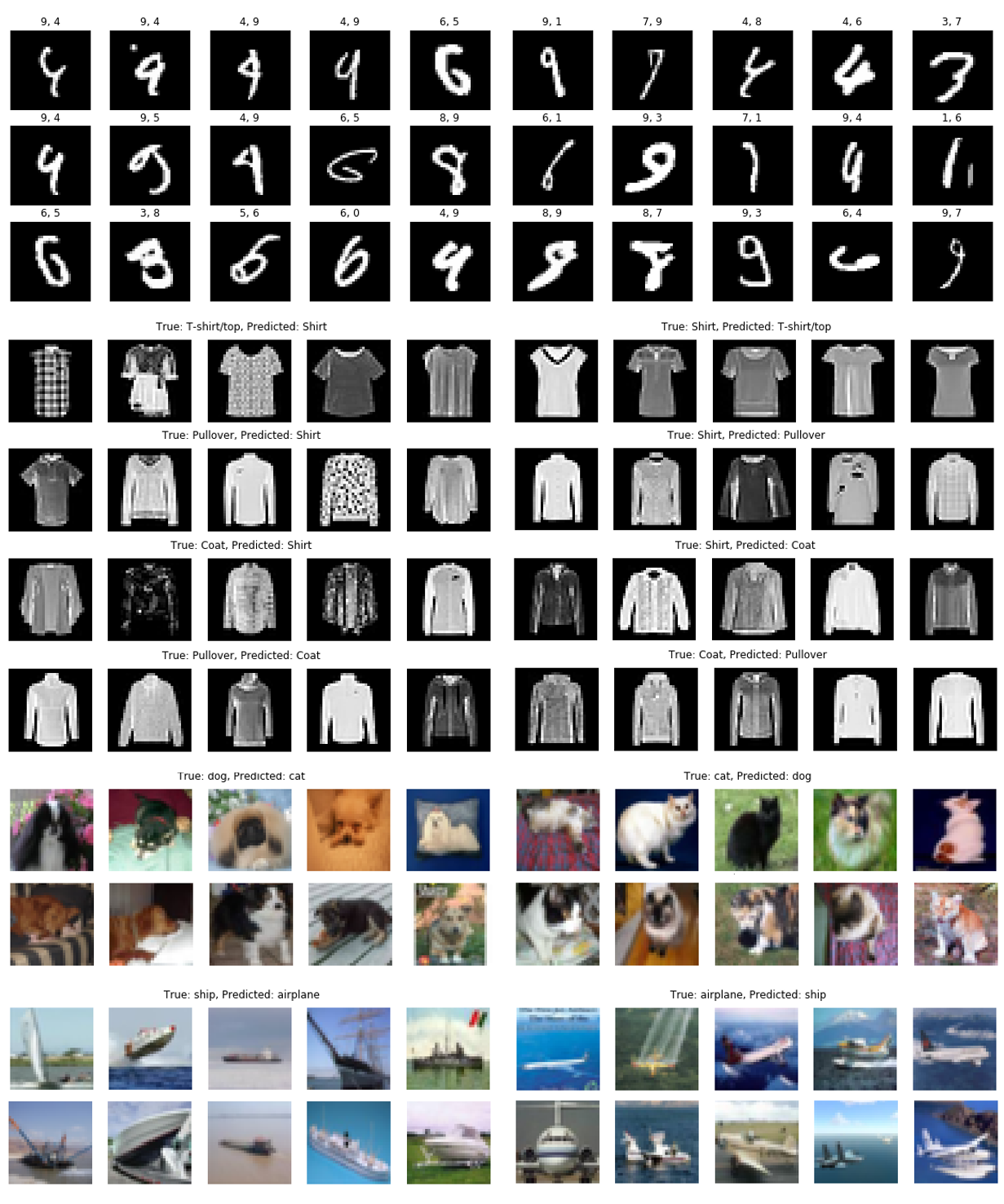
Figure 10: Representative misclassified images in three benchmarking datasets, where the first three rows show erroneous predictions in MNIST and the title above each sample indicates the ground-truth and prediction. The fourth and the seventh rows erroneous predictions of the “shirt" class and a confusing pair “pullover vs. coat" in Fashion MNIST, and the last four rows show two confusing pairs, “dog vs. cat" and “ship vs. airplane", in CIFAR-10.

Different Color Spaces. We report experimental results on CIFAR-10 with different color representations in Table 6. We consider three color spaces - RGB, YCbCr, and Lab. The three color channels are combined with different strategies: 1) three channels are taken as the input jointly; 2) each channel is taken as the input individually and all three channels are concatenated in module #3; 3) luminance and chrominance components are processed individually and concatenated in module #3. We see an advantage of processing one luminance channel (L or Y) and two chrominance channels (CbCr or ab) separately and then concatenate extracted features at the classification stage. This observation is consistent with our prior experience in color image processing.

Table 6: Comparison of classification accuracy (%) using different color representations on CIFAR-10.

	RGB	R,G,B	YCbCr	Y,CbCr	Lab	L,ab
Testing	68.90	69.96	68.74	71.05	67.05	71.37
Training	84.11	85.06	84.05	86.03	87.46	87.65

Weak supervision. Since PixelHop is a nonparametric learning method, it is scalable to the number of training samples. In contrast, LeNet-5 is a parametric learning method, and its model complexity is fixed regardless of the training data number. We compare the classification accuracies of LeNet-5 and PixelHop in Fig. 11, where only 1/4, 1/8, 1/16,1/32, 1/64, 1/128, of the original training dataset are randomly selected as the training data for MNIST, Fashion MNIST and CIFAR-10. After training, we apply the learned systems to 10,000 testing data as usual. As shown in Fig. 11, when the number of labeled training data is reduced, the classification performance of LeNet-5 drops faster than PixelHop. For the extreme case with 1/128 of the original training data size (i.e., 460 training samples), PixelHop outperforms LeNet-5 by 1.3% and 13.4% in testing accuracy for MNIST and Fashion MNIST, respectively. Clearly, PixelHop is more scalable than LeNet-5 against the smaller training data size. This could be explained by the fast convergence property of the Saab AC filters as discussed in Sec. 2.2.

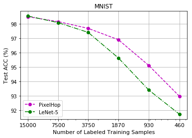
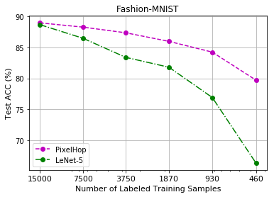
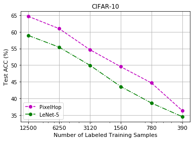
Figure 11: Comparison of testing accuracy (%) of LeNet-5 and PixelHop with different training sample numbers for MNIST, Fashion MNIST and CIFAR-10.

3.4 Performance Benchmarking between PixelHop and LeNet-5

We compare the training complexity and the classification performance of the LeNet-5 and the PixelHop method in this subsection. These two machine learning models share similar model complexity. We use the Lab color space to represent images in CIFAR-10 and build two PixelHop pipelines for the luminance and the chrominance spaces in modules #1 and #2 separately. Then, they are integrated in module #3 for final decision. For the LeNet-5, we train all networks using TensorFlow [20] with 50 epochs and a batch size of 32. The classic LeNet-5 architecture [17] was designed for the MNIST dataset. We use it for the Fashion MNIST dataset as well. We modify the network architecture slightly to handle color images in the CIFAR-10 dataset. The parameters of the original and the modified LeNet-5 are shown in Table 7. The modified LeNet-5 was originally proposed in [12].

Table 7: Comparison of the original and the modified LeNet-5 architectures.

Architecture	Original LeNet-5	Modified LeNet-5
1st Conv Layer Kernel Size	$5\times 5\times 1$	$5\times 5\times 3$
1st Conv Layer Kernel No.	$6$	$32$
2nd Conv Layer Kernel Size	$5\times 5\times 6$	$5\times 5\times 32$
2nd Conv Layer Kernel No.	$16$	$64$
1st FC Layer Filter No.	$120$	$200$
2nd FC Layer Filter No.	$84$	$100$
Output Node No.	$10$	$10$

We compare the classification performance of the PixelHop method with LeNet-5 and the feedforward-designed CNN (FF-CNN) [12] for all three datasets in Table 8. The FF-CNN method shares the same network architecture with LeNet-5. Yet, it determines the model parameters in the one-pass feedforward manner. As shown in Table 8, FF-CNN performs the worst while PixelHop⁺ performs the best in all datasets. The latter outperforms LeNet-5 by 0.05%, 0.6% and 3.94% for MNIST, Fashion MNIST and CIFAR-10, respectively. PixelHop also outperforms LeNet-5 for Fashion MNIST and CIFAR-10.

Furthermore, we compare the training time of LeNet-5 and PixelHop for all three datasets in Table 9. PixelHop takes less training time than LeNet-5 for all three datasets in a CPU, where the CPU is Intel(R) Xeon(R) CPU E5-2620 v3 at 2.40GHz. Although these comparisons are still preliminary, we do see that PixelHop can be competitive in terms of classification accuracy and training complexity.

Table 8: Comparison of testing accuracy (%) of LeNet-5, feedforward-designed CNN (FF-CNN), PixelHop and PixelHop⁺ for MNIST, Fashion MNIST and CIFAR-10.

Method	MNIST	Fashion MNIST	CIFAR-10
LeNet-5	99.04	91.08	68.72
FF-CNN	97.52	86.90	62.13
PixelHop	98.90	91.30	71.37
PixelHop+	99.09	91.68	72.66

Table 9: Comparison of training time of the LeNet-5 and the PixelHop method on the MNIST, the Fashion MNIST and the CIFAR-10 datasets.

Method	MNIST	Fashion MNIST	CIFAR-10
LeNet-5	$\sim$25 min	$\sim$25 min	$\sim$45 min
PixelHop	$\sim$15 min	$\sim$15 min	$\sim$30 min

4 Discussion

In this section, we first summarize the key ingredients of SSL in Sec. 4.1. Then, extensive discussion on the comparison of SSL and DL is made in Sec. 4.2 to provide further insights into the potential of SSL.

4.1 Successive Subspace Learning (SSL)

The PixelHop method presented in Sec. 2 offers a concrete example of SSL. Another design based on the SSL principle, called the PointHop method, was proposed in [14]. It is worthwhile to obtain a high-level abstraction for these methods. Generally speaking, an SSL system contains four ingredients:

1. successive near-to-far neighborhood expansion in multiple stages;

2. unsupervised dimension reduction via subspace approximation at each stage;

3. supervised dimension reduction via label-assisted regression (LAG); and

4. feature concatenation and decision making.

For the first ingredient, we compute the attributes of local-to-global neighborhoods of selected pixels in multiple stages successively. The main advantage of this design is that the attributes of near and far neighboring pixels can be propagated to the target pixel through local communication. The attributes can be gray-scale pixel values (for gray-scale images), the RGB pixel values (for color images), position coordinates (for point cloud data sets), etc. The attributes of near neighbors can be propagated in one hop while that of far neighbors can be propagated through multiple hops as well as through spatial pooling. For this reason, it is called the PixelHop (or PointHop) method. As the hop number becomes larger, we examine a larger neighborhood. Yet, the attribute dimension of a neighborhood will grow rapidly since it is proportional to the number of pixels in the neighborhood.

To control the speed of growing dimensions without sacrificing representation accuracy much, we need to find an approximate subspace in the second ingredient. Specifically, we exploit statistical correlations between attribute vectors associated with neighborhoods. PCA is a one-stage subspace approximation technique. When we consider successive subspace approximation in the SSL context, we adopt the Saab or the Saak transform to eliminate the sign confusion problem. This topic was discussed in [10], [11], [12]. PCA and Saab/Saak transforms are unsupervised dimension reduction techniques.

In earlier (or later) stages, the neighborhood size is smaller (or larger), the attribute vector dimension is smaller (or larger), and the number of independent neighborhoods is larger (or smaller). All of them can contribute to classification accuracy. For an object class, the attributes of its near and far neighbors follow a certain distribution. We use the label information at all stages to achieve further dimension reduction. The label-assisted regression (LAG) unit was developed in Sec. 2.3 for this purpose. This corresponds to the third ingredient.

For the last ingredient, dimension-reduced attributes from all stages are concatenated to form the ultimate feature vector and a multi-class classifier is trained for the classification task.

Table 10: Similarities of SSL and DL.

	SSL	DL
Attributes collection	Successively growing neighborhoods	Gradually enlarged receptive fileds
Attributes processing	Trade spatial for spectral dimensions	Trade spatial for spectral dimensions
Spatial dim. reduction	Spatial pooling	Spatial pooling

4.2 Comparison of DL and SSL

SSL and DL have some high-level concept in common, yet they are fundamentally different in their models, training processes and training complexities. We list similarities of SSL and DL in Table 10.

Similarities reside in the high-level principle. Both collect attributes in the pixel domain by employing successively growing neighborhoods. Both trade spatial-domain patterns for spectral components using convolutional filters. As the neighborhood becomes larger, the dimension of spectral components become larger. Due to significant neighborhood overlapping, there exists strong redundancy between neighborhoods of adjacent pixels. The spatial pooling is adopted by reducing such redundancy.

Table 11: Differences of SSL and DL.

	SSL	DL
Model expandability	Non-parametric model	Parametric model
Incremental learning	Easy	Difficult
Model architecture	Flexible	Networks
Model interpretability	Easy	Difficult
Model parameter search	Feedforward design	Backpropagation
Training/testing complexity	Low	High
Spectral dim. reduction	Subspace approximation	Number of filters
Task-independent features	Yes	No
Multi-tasking	Easy	Difficult
Incorporation of priors and constraints	Easy	Difficult
Weak supervision	Easy	Difficult
Adversarial Attacks	Difficult	Easy

Next, we show differences between SSL and DL in Table 11 and elaborate them below.

• Model expandability
  DL is a parametric learning method. One selects a fixed network architecture to begin with. The superior performance of DL is attributed to a very large model size, where the number of model parameters is typically larger than the number of training samples, leading to an over-parameterized network. This could be a waste of resource. Traditional parametric learning methods do not have enough model parameters to deal with datasets of a larger number of samples with rich diversity. SSL adopts a non-parametric model. It is flexible to add and/or delete filters at various units depending on the size of the input dataset. SSL can handle small and large datasets using an expandable model. This is especially attractive for edge computing. Its model complexity can be adjusted flexibly based on hardware constraints with graceful performance tradeoff.

• Incremental learning
  It is challenging to adapt a trained DL model to new data classes and samples. Since SSL employs a non-parametric model, we can check whether existing Saab filters can express the new data well. If not, we can add more Saab filters in the unsupervised dimension reduction part. Furthermore, we can expand the regression matrix to accommodate new classes.

• Model architecture
  DL demands a network architecture that has an end node at which a cost function has to be defined. This is essential to allow BP to train the network parameters. In contrast, the architecture of an SSL design is more flexible. We can extract rich features from processing units in multiple stages. Furthermore, we can conduct ensemble learning on these features.

• Model interpretability
  The DL model is a black-box tool. Many of its properties are not well understood. The SSL model is a white-box, which is mathematically transparent.

• Model parameter search
  DL determines model parameters using an end-to-end optimization approach, which is implemented by BP. SSL adopts unsupervised and supervised dimension reduction techniques to zoom into an effective subspace for feature extraction. The whole pipeline is conducted in a one-pass feedforward fashion.

• Training and testing complexity
  DL demands a lot of computing resources in model training due to BP. As the number of layers goes extremely deep (say, 100 and 150 layers), the inference can be very expensive as well. The training complexity of SSL is significantly lower since it is a one-pass feedforward design. Its testing complexity is determined by the stage number. If the number of stages is small, inference can be done effectively.

• Spectral dimension reduction
  Although DL and SSL both use convolutional operations, they have different meanings. Convolutions in DL are used to transform one representation to another aiming at end-to-end optimization of the selected cost function for the network. Convolutions in SSL are used to find projections onto principal components of the subspace.

• Task-independent features
  DL uses both input images and output labels to determine system parameters. The derived features are task dependent. SSL contains two feature types: task-independent features and task-dependent features. The features obtained by unsupervised dimension reduction are task-independent while those obtained by supervised dimension reduction are task-dependent.

• Multi-tasking
  DL can integrate the cost functions of multiple tasks and define a new joint cost function. This joint cost function may not be optimal with respect to each individual task. SSL can obtain a set of task-independent features and feed them into different LAG units and different classifiers to realize multi-tasking.

• Incorporation of priors and constraints
  DL may add new terms to the original cost function, which corresponds to priors and constraints. The impact of the modified cost function on the learning system is implicit and indirect. SSL can use priors and constraints to prune attributes of small and large neighborhoods directly before they are fed into the classifier.

• Weak supervision
  A large number of labeled data are needed to train DL models. Data augmentation is often used to create more training samples. It was shown in Sec. 3 that SSL outperforms DL in the weak supervision case. This could be attributed to that the unsupervised dimension reduction process in successive PixelHop units do not demand labels. Labels are only needed in the LAG units and the training of a classifier. Besides, we may adopt a smaller SSL model in the beginning. Then, we can grow the model size by adding more confident test samples to the training dataset.

• Adversarial attacks
  It is well known that one can exploit the DL network model to find a path from the output decision space to the input data space. Then, a decision outcome can be changed by adding small perturbations to the input. The perturbation can be so small that humans may not be able to see. As a result, two almost identical images will result in different predictions. This is one major weakness of DL networks. In SSL, we expect that weak perturbation can be easily filtered out by PCA, and it is challenging for attackers to conduct similar attacks.

5 Conclusion and Future Work

A successive subspace Learning (SSL) methodology was introduced and the PixelHop method was proposed in this work. In contrast with traditional subspace methods, SSL examines the near- and far-neighborhoods of a set of selected pixels. It uses the training data to learn three sets of parameters: 1) Saab filters for unsupervised dimension reduction in the PixelHop unit, 2) regression matrices for supervised dimension reduction in the LAG unit, and 3) parameters required by the classifier. Extensive experiments were conducted on MNIST, Fashion MNIST and CIFAR-10 to demonstrate the superior performance of the PixelHop method in terms of classification accuracy and training complexity.

SSL is still at its infancy. There exist rich opportunities for further development and extension. A couple of them are mentioned below. First, generative adversarial networks (GAN) have been developed as generative models, and they find applications in style transfer, domain adaptation, data augmentation, etc. It seems feasible to develop an SSL-based generative model. That is, we need to ensure that attribute vectors associated with neighborhoods of various sizes of the source-domain and target-domain images share the same distribution. Second, we would like to investigate SSL-based contour/edge detection and image segmentation techniques. Historically, contour/edge detection and image segmentation played an important role in low-level computer vision. Their importance drops recently due to the flourish of DL. Yet, any feedforward computer vision pipeline should benefit from these basic operations. Based on this foundation, we can tackle with object detection and object recognition problems using the SSL framework.

References

- [1] Matthew Turk and Alex Pentland. Eigenfaces for recognition. Journal of cognitive neuroscience, 3(1):71–86, 1991.
- [2] Thierry Bouwmans. Subspace learning for background modeling: A survey. Recent Patents on Computer Science, 2(3):223–234, 2009.
- [3] Hans-Peter Kriegel, Peer Kröger, and Arthur Zimek. Clustering high-dimensional data: A survey on subspace clustering, pattern-based clustering, and correlation clustering. ACM Transactions on Knowledge Discovery from Data (TKDD), 3(1):1, 2009.
- [4] Haiping Lu, Konstantinos N Plataniotis, and Anastasios N Venetsanopoulos. A survey of multilinear subspace learning for tensor data. Pattern Recognition, 44(7):1540–1551, 2011.
- [5] Quanquan Gu, Zhenhui Li, and Jiawei Han. Joint feature selection and subspace learning. In Twenty-Second International Joint Conference on Artificial Intelligence, 2011.
- [6] Kaiye Wang, Ran He, Liang Wang, Wei Wang, and Tieniu Tan. Joint feature selection and subspace learning for cross-modal retrieval. IEEE transactions on pattern analysis and machine intelligence, 38(10):2010–2023, 2015.
- [7] Jing Wang, Zhenyue Zhang, and Hongyuan Zha. Adaptive manifold learning. In Advances in neural information processing systems, pages 1473–1480, 2005.
- [8] Tong Lin and Hongbin Zha. Riemannian manifold learning. IEEE Transactions on Pattern Analysis and Machine Intelligence, 30(5):796–809, 2008.
- [9] Tsung-Han Chan, Kui Jia, Shenghua Gao, Jiwen Lu, Zinan Zeng, and Yi Ma. Pcanet: A simple deep learning baseline for image classification? IEEE Transactions on Image Processing, 24(12):5017–5032, 2015.
- [10] C.-C. Jay Kuo. Understanding convolutional neural networks with a mathematical model. Journal of Visual Communication and Image Representation, 41:406–413, 2016.
- [11] C.-C. Jay Kuo and Yueru Chen. On data-driven Saak transform. Journal of Visual Communication and Image Representation, 50:237–246, 2018.
- [12] C-C Jay Kuo, Min Zhang, Siyang Li, Jiali Duan, and Yueru Chen. Interpretable convolutional neural networks via feedforward design. Journal of Visual Communication and Image Representation, 60:346–359, 2019.
- [13] C.-C. Jay Kuo. The CNN as a guided multilayer RECOS transform [lecture notes]. IEEE Signal Processing Magazine, 34(3):81–89, 2017.
- [14] Min Zhang, Haoxuan You, Pranav Kadam, Shan Liu, and C-C Jay Kuo. Pointhop: An explainable machine learning method for point cloud classification. arXiv preprint arXiv:1907.12766, 2019.
- [15] Corinna Cortes and Vladimir Vapnik. Support-vector networks. Machine learning, 20(3):273–297, 1995.
- [16] Leo Breiman. Random forests. Machine learning, 45(1):5–32, 2001.
- [17] Yann Lecun, Léon Bottou, Yoshua Bengio, and Patrick Haffner. Gradient-based learning applied to document recognition. In Proceedings of the IEEE, pages 2278–2324, 1998.
- [18] Han Xiao, Kashif Rasul, and Roland Vollgraf. Fashion-mnist: a novel image dataset for benchmarking machine learning algorithms. arXiv preprint arXiv:1708.07747, 2017.
- [19] Alex Krizhevsky and Geoffrey Hinton. Learning multiple layers of features from tiny images. Technical report, Citeseer, 2009.
- [20] Martín Abadi, Ashish Agarwal, Paul Barham, Eugene Brevdo, Zhifeng Chen, Craig Citro, Greg S. Corrado, Andy Davis, Jeffrey Dean, Matthieu Devin, Sanjay Ghemawat, Ian Goodfellow, Andrew Harp, Geoffrey Irving, Michael Isard, Yangqing Jia, Rafal Jozefowicz, Lukasz Kaiser, Manjunath Kudlur, Josh Levenberg, Dan Mané, Rajat Monga, Sherry Moore, Derek Murray, Chris Olah, Mike Schuster, Jonathon Shlens, Benoit Steiner, Ilya Sutskever, Kunal Talwar, Paul Tucker, Vincent Vanhoucke, Vijay Vasudevan, Fernanda Viégas, Oriol Vinyals, Pete Warden, Martin Wattenberg, Martin Wicke, Yuan Yu, and Xiaoqiang Zheng. TensorFlow: Large-scale machine learning on heterogeneous systems, 2015. Software available from tensorflow.org.