Entanglement measures of bipartite quantum gates and their thermalization
under arbitrary interaction strength

Abstract

Entanglement properties of bipartite unitary operators are studied via their local invariants, namely the entangling power $e_{p}$ and a complementary quantity, the gate typicality $g_{t}$. We characterize the boundaries of the set $K_{2}$ representing all two-qubit gates projected onto the plane $(e_{p},g_{t})$ showing that the fractional powers of the swap operator form a parabolic boundary of $K_{2}$, while the other bounds are formed by two straight lines. In this way a family of gates with extreme properties is identified and analyzed. We also show that the parabolic curve representing powers of swap persists in the set $K_{N}$, for gates of higher dimensions ($N>2$). Furthermore, we study entanglement of bipartite quantum gates applied sequentially $n$ times and analyze the influence of interlacing local unitary operations, which model generic Hamiltonian dynamics. An explicit formula for the entangling power a gate applied $n$ times averaged over random local unitary dynamics is derived for an arbitrary dimension of each subsystem. This quantity shows an exponential saturation to the value predicted by the random matrix theory (RMT), indicating “thermalization” in the entanglement properties of sequentially applied quantum gates that can have arbitrarily small, but nonzero, entanglement to begin with. The thermalization is further characterized by the spectral properties of the reshuffled and partially transposed unitary matrices.

I Introduction

A clutch of quantities such as state entanglement, operator entanglement, operator scrambling, out-of-time-ordered correlators, and various measures of mutual information are being currently actively pursued as a means to understand information transport in complex quantum systems and to characterize quantum chaos Swingle et al. (2016); Nahum et al. (2017); He and Lu (2017); Zhou and Luitz (2017); Seshadri et al. (2018); Hosur et al. (2016); Chan et al. (2018); von Keyserlingk et al. (2018). Entangling power of the time evolution operator has been studied since its introduction as a state independent measure Zanardi et al. (2000); Zanardi (2001); Wang and Zanardi (2002), and is the average entanglement an operator produces when acting on product, unentangled, states. On the other hand, operator entanglement quantifies to what extent a given operator, treated as a vector in the Hilbert-Schmidt space of operators, is close to the tensor product Życzkowski and Bengtsson (2004). Operator entanglement and entangling power have both recently been applied to many-body systems, in particular in the context of spin-chains and conformal field theories Zhou and Luitz (2017); Dubail (2017); Pal and Lakshminarayan (2018), where it has been found useful to distinguish between integrable and non-integrable systems as well as in the analysis of the many-body-localization transition.

The study of the operator entanglement and entangling power of the time evolution operator $\exp(-iHt/\hbar)$, or its time-ordered version if the Hamiltonian $H$ is a function of time, is of fundamental import in the growth of subsystem entropy and complexity of closed systems ranging from two large bipartite systems to quantum spins on lattices Lubkin and Lubkin (1993); Miller and Sarkar (1999); Bandyopadhyay and Lakshminarayan (2002); Fujisaki et al. (2003); Bandyopadhyay and Lakshminarayan (2004); Demkowicz-Dobrzański and Kuś (2004); Linden et al. (2009); Chaudhury et al. (2009); Neill and et al. (2016); Lakshminarayan et al. (2016); Schuch et al. (2008); Abreu and Vallejos (2007); Calabrese (2018); Bertini et al. (2019a); Bravyi (2007); Petitjean and Jacquod (2006); Trail et al. (2008); Pulikkottil et al. (2020). The action of this time-evolution operator on unentangled states generally creates multipartite entanglement. From another perspective, the Heisenberg evolution results in operator entanglement and scrambling in the space of operators Nahum et al. (2017); Chan et al. (2018); von Keyserlingk et al. (2018); Moudgalya et al. (2019). A central aspect of this paper is the study of dynamics of quantum entanglement in products of unitary matrices, which are interpreted as time-evolution operators, with the number of terms in the product playing the role of discrete time.

From the point of view of quantum computing Nielsen and Chuang (2000), gate operations ordered in time are the source of information transfer. Products of unitary operators are therefore natural objects to study as they form building blocks for quantum algorithms. Random quantum circuits with random unitary operators providing interaction among qubits have been studied in this context Emerson et al. (2003); Harrow and Low (2009); Kondratiuk and Życzkowski (2013). They are known to be approximate unitary $t-$designs that simulate Haar distributed unitaries Dankert et al. (2009); Brandao et al. (2016). Models of random quantum circuits have been studied in many other contexts including randomised benchmarking Emerson et al. (2005), entanglement spreading, scrambling and many-body localization Chan et al. (2018); von Keyserlingk et al. (2018); Sünderhauf et al. (2018).

Random quantum circuits are constructed by arbitrarily choosing pairs of quNits between which the interactions are described by random unitary matrices Collins et al. (2010), typically Haar distributed. In a departure from this standard formalism, we are primarily interested in the role of local random unitaries with a tensor product structure, which interlace sequential dynamics described by a fixed non-local gate $V$ acting on a bipartite system. Such a bipartite structure could form a building block for more general random quantum circuits with fixed, possibly atypical, nonlocal gates and random or generic local interaction.

Another setting in which products of nonlocal unitaries interspersed with local ones arise naturally are in kicked systems which are being extensively used. In this context, the object of interest could be powers of the Floquet operator $U$ Bandyopadhyay and Lakshminarayan (2002, 2004); Demkowicz-Dobrzański and Kuś (2004); Pal and Lakshminarayan (2018); Zhou and Luitz (2017), or if the local Hamiltonians are non-autonomous, products of propagators across consecutive periods of the kicking. In particular, let

$$H=H_{A}(t)\otimes\mathbb{1}_{B}+\mathbb{1}_{A}\otimes H_{B}(t)+H_{AB}\sum_{n=-\infty}^{\infty}\delta(t/\tau-n),$$ (1)

be the Hamiltonian and

$$u_{Aj}=\mathcal{T}e^{-i\int_{(j-1)\tau}^{j\tau}H_{A}(t)dt},$$ (2)

where $\mathcal{T}$ denotes time ordering. The time evolution operator between (just before) kicks $j-1$ and $j$ is

$$\mathcal{U}_{j}=\left(u_{A\,j}\otimes u_{B\,j}\right)\,U$$ (3)

where $U=e^{-i\tau H_{AB}}$ arises from the non-local interaction at time $j\tau$ and $u_{Bj}$ is defined similar to $u_{Aj}$. This is the Floquet operator across the time period $\tau$ between the $j-1$ and $j^{th}$ kicks. The propagator across $n$ kicks is

$$\mathcal{U}^{(n)}=\mathcal{T}\prod_{j=1}^{n}\mathcal{U}_{j}=\mathcal{T}\prod_{j=1}^{n}(u_{A_{j}}\otimes u_{B_{j}})\,U.$$ (4)

The brackets around the “power” $n$ is to indicate that there are $n$ different terms in the product generally and the time ordering will be assumed below and hence not explicitly indicated. Most systems that have been studied are such the $u_{Aj}$ and $u_{Bj}$ are independent of $j$, that is the local Hamiltonians are autonomous. This leads to a time-periodic system with $\mathcal{U}$ as the Floquet operator and we are then interested in the powers $\mathcal{U}^{n}$. However, a product of unitary operators with different local operators occur in contexts such as time-dependent quenches, for example see the study Mishra and Lakshminarayan (2014) for quenched kicked Ising spin chains.

Past work has shown that while bipartite local unitaries $u_{A}\otimes u_{B}$ have no entangling power, layering or interspersing them in time with entangling gates provides a crucial role for random local unitaries Jonnadula et al. (2017); Mandarino et al. (2018). Local unitary gates are easier to apply in an experiment and are thus naturally “cheaper” than nonlocal entangling gates. However, the role of such local unitary gates in creating Haar random unitaries or in achieving thermalization is to our knowledge not sufficiently explored. Specifically, we focus here on the thermalization of the entangling power of the unitary operator $\mathcal{U}^{(n)}$, as defined in Eq. (4), where thermalization in understood to mean that after a certain number $n$ of interaction times the quantities studied reach the typical values corresponding to the Haar average over the unitary group. We find that the natural quantities to study are indeed the entangling power, $e_{p}$, and a complementary quantity defined in Jonnadula et al. (2017), as the “gate typicality”, $g_{t}$. In particular, we are interested in the entangling power and gate typicality of $\mathcal{U}^{(n)}$. The importance of the operator entanglement and entangling power stems from their invariance under local unitary operations and hence measure the essential nonlocal content of the process.

This paper contains two complementary but in some ways distinct motivations and results, which for the sake of the convenience of the reader we enumerate below.

1. The first part of this paper is dedicated to visualizing the entanglement landscape of bipartite gates in dimensions $N^{2}$, in terms of entangling power and gate typicality. For the case of qubits, $N=2$, the picture is complete and we show in detail the various gates that make up the “phase-space” spanned by these two local invariants. We prove the existence of a boundary consisting exclusively of the fractional powers of the swap operator. Of special interest are gates that maximize entangling power, in the sense that they attain bounds set by the dimensionality $N$. It is known that for two-qubit systems such a gate does not exist Higuchi and Sudbery (2000a), while the maximal entangling power is attained for cnot and related gates Zanardi et al. (2000); Jonnadula et al. (2017).

2. If the first part is about the “kinematics” of the entangling power and gate typicality, the second is a study of its “dynamics”, via the entangling power of the products of unitaries. We generalize earlier results Jonnadula et al. (2017) for equal subsystem dimensionality to the important case when the two subsystems could be of different dimensions. In a central result in this context, we demonstrate the exponentially fast thermalization of the average entangling power of $\mathcal{U}^{(n)}=\Pi_{j=1}^{n}\mathcal{U}_{j}$ with time, to that of a typical unitary operator. Furthermore, we show that there are signatures of such a thermalization in the spectra of the opeators obtained by reshuffing and partial transposition (both permutations) of the time-evolution operator.

Thus the second part of this work shows the thermalization of the entangling power of $U$ under time evolution with non-autonomous local evolutions. Such exponential saturation also seems to provide excellent approximations in the case of autonomous Floquet systems Jonnadula et al. (2017) whose dimensions are not very small, although the circumstances under which this holds needs further investigation. Thus we expect applications not only for coupled chaotic systems such as the kicked top and the kicked rotor, but also to many-body systems such as the kicked and tilted field Ising models Zhou and Luitz (2017); Pal and Lakshminarayan (2018). The exponential approach of the average entangling power of $\mathcal{U}^{(n)}$ to the Haar average is determined solely by $e_{p}(U)$, the entangling power of the interaction. This demonstrates that any nonzero value of the entangling power, however small, is sufficient to thermalize its powers interspersed with random local operators.

Apart from the entangling power, the gate typicality Jonnadula et al. (2017) also has a simple exponential approach to the global RMT average, depending solely upon the $g_{t}(U)$, the gate typicality of the interaction. In fact, this formed an important basis for the introduction of this quantity that is naturally singled out. In contrast, the thermalization of other local invariants, such as the operator entanglement, are sums of exponentials with different rates. The extremal values of the gate-typicality, $g_{t}=0$ and $g_{t}=1$, correspond to local gates and the swap operator, respectively, while the average value, $g_{t}=1/2$ (for equal subsystem dimensions), characterizes the Haar average over the entire set of bipartite unitary gates. Thus the entangling power and gate typicality are local invariants associated with the interaction $U$ that determine the complexity of products such as $\Pi_{j=1}^{n}\mathcal{U}_{j}$.

The paper is organized as follows. Section (II) will introduce in detail all the relevant quantities, including operator entanglement and entangling power. Section (III) studies the allowed region of the invariants for the case of two qubits. We study this via the entangling power, gate typicality ($e_{p},g_{t}$) phase space and establish the boundaries of the allowed gates. Section (IV) discusses some special gates such as the Fourier and the fractional powers of swap in arbitrary dimensions, and give partial results for qutrits as well as conjecture that the fractional powers of swap form a boundary for all quNits. Finally in Section (V) we study time evolution and prove the thermalization of entangling power (and gate typicality) under certain conditions. Here, we generalize our earlier result obtained in Jonnadula et al. (2017), referring to Appendix C for an elegant proof. Finally, we provide examples wherein the thermalization can be seen via approach of the partial transposed and reshuffled operators to the Girko circular law Girko (1985) and their squared singular values to the Marcenko-Pastur distribution Marčenko and Pastur (1967). Section (VI) provides a summary and outlook.

II Local Invariants of operators: Entangling power and gate typicality

II.1 Two sets of local unitary invariants and operator entanglement

Consider a unitary operator $U$ acting on the bipartite space ${\cal H}_{N}^{A}\otimes{\cal H}_{N}^{B}$ of two parts labeled $A$ and $B$. For simplicity we restrict attention to spaces whose dimensions are equal (and to $N$). The generalization to unequal dimensions is treated in Appendix A. Operators such as $U$ may be “gates” in the language of quantum circuits, or just quantum propagators describing evolution over some finite time. The fact that $U$ need not be of a product form $u_{A}\otimes u_{B}$, with $u_{A,B}$ acting on ${\cal H}_{N}^{A,B}$ in general implies that it is usually capable of creating entanglement when it acts on unentangled states. Let the operator Schmidt decomposition of $U$ be Życzkowski and Bengtsson (2004)

$$U=\sum_{j=1}^{N^{2}}\sqrt{\lambda_{j}}\,M_{A_{j}}\otimes M_{B_{j}},$$ (5)

where the operators on the individual spaces $M_{A_{j}}$ and $M_{B_{j}}$ are in general not unitary themselves, but form an orthonormal basis for operators on their respective spaces, $\mbox{tr}(M_{A_{j}}^{\dagger}M_{A_{k}})=\mbox{tr}(M_{B_{j}}^{\dagger}M_{B_{k}})=\delta_{jk}$, where $\delta_{jk}$ is the Kronecker delta. The Schmidt vector $\lambda=\{\lambda_{j}\}_{j=1}^{N^{2}}$ is determined by singular values of the reshuffled matrix $U^{R}$ – see Appendix A. Note that $\lambda$ is invariant under local unitary operations. Unitarity of $U$ implies that

$$\frac{1}{N^{2}}\sum_{j=1}^{N^{2}}\lambda_{j}=1,$$ (6)

so the rescaled vector of Schmidt ceofficients, $\{\lambda_{i}/N^{2}\}$, can be treated as a discrete probability measure that characterizes the nonlocality of the operator $U$. To elaborate let

$$U\rightarrow U^{\prime}=(u_{A_{1}}\otimes u_{B_{1}})\,U\,(u_{A_{2}}\otimes u_{B_{2}}),$$ (7)

where $u_{A_{j},B_{k}}$ are “local” unitary operators. In the language of dynamics, they constitute single-particle evolutions. The content of nonlocality of $U$ and $U^{\prime}$ is identical and hence the measures characterizing their nonlocality must be the same. In the case of states, this constitutes the condition that all entanglement measures be local unitary invariants. It is clear from the definition of the operator Schmidt decomposition that the set $\{\lambda_{i}\}$ are $N^{2}$ such invariants, as $M_{A_{j}}\rightarrow u_{A_{1}}M_{A_{j}}u_{A_{2}}$ also constitute an operator basis consisting of orthonormal operators, and similarly for $M_{B_{j}}$.

Another set of $N^{2}$ invariants are constructed from the operator Schmidt decomposition of the operator product $US$ where $S$ is the swap (or flip) operator defined as

$$S|\phi_{A}\rangle|\phi_{B}\rangle=|\phi_{B}\rangle|\phi_{A}\rangle,\,\text{or}\,S(u_{A}\otimes u_{B})S=u_{B}\otimes u_{A},$$ (8)

for arbitrary states $|\phi_{A,B}\rangle$ and operators $u_{A,B}$. Let

$$US=\sum_{j=1}^{N^{2}}\sqrt{\mu_{j}}\,\tilde{M}_{A_{j}}\otimes\tilde{M}_{B_{j}},$$ (9)

be its Schmidt decomposition. As $S$ is unitary we also have that

$$\frac{1}{N^{2}}\sum_{j=1}^{N}\mu_{j}=1.$$ (10)

That the set $\{\mu_{i}\}$ constitute $N^{2}$ invariants follows from the observation that

$$\begin{split}U^{\prime}S&=(u_{A_{1}}\otimes u_{B_{1}})\,U\,(u_{A_{2}}\otimes u_{B_{2}})S\\ &=(u_{A_{1}}\otimes u_{B_{1}})\,US\,(u_{B_{2}}\otimes u_{A_{2}}),\end{split}$$ (11)

and hence the Schmidt eigenvalues of $US$, the $\mu_{i}$, are the same as the Schmidt eigenvalues of $U^{\prime}S$. The product $SU$ does not produce any newer invariants.

This paper is focused on these two sets of invariants and quantities derived from them. In particular, their moments and entropies provide measures of how nonlocal the operator $U$ is, leading to a class of operator entanglement entropies. Here, we will be concerned with the entropies related to the second moments, given by,

$$E(U)=1-\frac{1}{N^{4}}\sum_{j=1}^{N^{2}}\lambda_{j}^{2},\;\;\text{and}\;E(US)=1-\frac{1}{N^{4}}\sum_{j=1}^{N^{2}}\mu_{j}^{2}.$$ (12)

$E(U)$ and $E(US)$ are the linear operator entanglement entropies of the operators $U$ and $US$ respectively. They take values in $[0,1-1/N^{2}]$, and $E(U)=0$ iff $U$ is a local product operator.

II.2 Entangling power and a complementary quantity

Notice that $E(U)$ and $E(US)$ are in some sense complementary quantities, as for a product operator,

$$E(u_{A}\otimes u_{B})=0,\;\text{while}\;E((u_{A}\otimes u_{B})S)=E(S)=1-\frac{1}{N^{2}}.$$ (13)

The last relation follows from the Schmidt decomposition of $S$ which is

$$S=\sum_{i,k=1}^{N}e_{ik}\otimes e_{ki},\;\text{where}\;e_{ik}=|i\rangle\langle k|.$$ (14)

Here $\{|i\rangle,\,1\leq i\leq N\}$ denotes any orthogonal basis and hence represents a continuous family of possible Schmidt decompositions, each with $\lambda_{j}=1$ for $1\leq j\leq N^{2}$. The swap operator has the maximum operator entanglement entropy according to any measure of entropy, including the linear one, $E(S)$ as above. Thus if $E(U)=E(S)$ the operator is $U$ maximally entangled. The complementary quantity $E(US)$ vanishes in the case of the swap gate, that is, $E(US)=E(S^{2})=0$. In fact, linear combinations of these two complementary quantities give rise to two measures that are extensively discussed in this paper.

One of the two measures we look at is the well-studied “entangling power”. The entangling power $e_{p}(U)$ Zanardi et al. (2000); Zanardi (2001) of an operator $U\in\mathcal{H}^{N}_{A}\otimes\mathcal{H}^{N}_{B}$ is defined as the average entanglement created when $U$ acts on product state $|\psi_{A}\rangle|\psi_{B}\rangle$ sampled according to the Haar measure on the individual spaces:

$$e_{p}(U)=\left(\frac{N+1}{N-1}\right)\,\overline{\mathcal{E}(U|\psi_{A}\rangle|\psi_{B}\rangle)}^{\psi_{A},\psi_{B}}.$$ (15)

Here the entanglement measure is the linear entropy $\mathcal{E}(|\psi\rangle)=1-\mbox{tr}_{A}(\rho^{2}_{A})$ and $\rho_{A}$ is the reduced density matrix $\mbox{tr}_{B}(|\psi\rangle\langle\psi|)$. It has been shown in Zanardi (2001) that for any gate $U$ its entangling power can be expressed by the linear operator entanglement entropy,

$$e_{p}(U)=\frac{1}{E(S)}\left[E(U)+E(US)-E(S)\right].$$ (16)

The range of $e_{p}(U)$ is,

$$0\leq e_{p}(U)\leq 1,$$ (17)

which follows from the fact that the maximum value of $E(U)$ is $E(S)$. We have rescaled the definition of $e_{p}(U)$ from that originally defined in Zanardi et al. (2000), so that the maximum value is simply $1$ independent of $N$.

If $e_{p}(U)=0$ then $U$ is either a product of local operators or locally equivalent to the swap. The fact that swap does not create any entanglement when acting on product states leads to $e_{p}(S)=0$, but that it is highly nonlocal is reflected in its operator entanglement being maximum. This is one motivation for introducing the complementary quantity

$$g_{t}(U):=\frac{1}{2E(S)}\left[E(U)-E(US)+E(S)\right]$$ (18)

where $g_{t}$ is referred to as gate typicality in Jonnadula et al. (2017). The range of $g_{t}(U)$ is

$$0\leq g_{t}(U)\leq 1,$$ (19)

and $g_{t}(U)=1$ iff $U$ is the swap or is locally equivalent to the swap. Again, we have rescaled $g_{t}$ from the original definition in Jonnadula et al. (2017) by a factor of $2$ for complete parity with $e_{p}$.

Thus while $e_{p}$ does not distinguish the local operators from the swap, $g_{t}$ does. It turns out that rather than discussing the pair $\{E(U),E(US)\}$ in several settings it seems more natural to work in the plane $\{e_{p}(U),g_{t}(U)\}$. The average of these measures when $U$ is sampled uniformly from the space of unitary matrices with respect to the Haar measure constitutes the average over the circular unitary ensemble (CUE) and reads

$$\overline{E}=\overline{e_{p}}=\frac{N^{2}-1}{N^{2}+1}=\frac{E(S)}{2-E(S)},\;\;\overline{g_{t}}=\frac{1}{2}.$$ (20)

As the scale is set so that $g_{t}\in[0,1]$, and the Haar average reads $1/2$ we see that both classes of local gates and gates locally equivalent to swap are equally non-typical. The fact that $\overline{E}$ and $\overline{e_{p}}$ are close to the maximal possible value indicates that a typical Haar unitary gate has strong entangling properties Musz et al. (2013), in analogy to the known fact that a generic bipartite pure state is strongly entangled Lubkin and Lubkin (1993); Życzkowski and Sommers (2001).

Computation of the operator Schmidt decomposition and the operator entanglements follows from suitable permutations of the unitary matrix. If $\langle i\alpha|U|j\beta\rangle=\langle ij|U^{R}|\alpha\beta\rangle$ and $\langle i\alpha|U|j\beta\rangle=\langle j\alpha|U^{T_{A}}|i\beta\rangle$ denote the reshuffling (also referred to as realignment) and the partial transpose operations respectively, we may define the following density matrices Życzkowski and Bengtsson (2004):

$$\rho_{R}(U)=\frac{1}{N^{2}}U^{R}U^{R\dagger},\;\;\rho_{T}(U)=\frac{1}{N^{2}}U^{T_{A}}U^{T_{A}\dagger}.$$ (21)

Their linear entropies are given by

$$E(U)=1-\frac{1}{N^{4}}\mbox{tr}\left(U^{R}U^{R\,\dagger}\right)^{2},$$ (22)

and

$$E(US)=1-\frac{1}{N^{4}}\mbox{tr}\left(U^{T_{A}}U^{T_{A}\,\dagger}\right)^{2}.$$ (23)

The operational interpretations of these quantities in terms of state entanglement of the equivalent $4$-party system is elaborated in Appendix A, including the generalization to the case of unequal subsystem dimensionality.

Note that if $U^{R}$ is also unitary then $E(U)=E(S)$ is the maximum possible. Unitary operators whose reshuffling is also unitary have recently been called dual-unitaries due to their appearance in lattice models with space-time duality Akila et al. (2016); Bertini et al. (2019a, b). This class contains, for instance, the discrete Fourier transform $F_{N^{2}}$, for which all coefficients in the operator Schmidt decomposition are equal Nielsen et al. (2003); Musz et al. (2013). This dual-unitary property allows for special many-body systems built out of such unitaries to be solvable in some sense Bertini et al. (2020); Gutkin et al. ; Piroli et al. (2020), although they can be non-integrable. It is indeed interesting that such unitaries are also maximally entangled in the operator entanglement sense. A way to generate ensembles of dual-unitaries has been presented in Rather et al. (2019).

If $U^{T_{A}}$ is also unitary, apart from $U^{R}$, then $E(US)=E(S)$. Such a matrix $U$, called “$2$-unitary” Goyeneche et al. (2015), saturates the maximum of entangling power, set to unity by our normalization. As discussed in Appendix A any two-unitary matrix of order $N^{2}$ corresponds to a two-uniform state state of four quNits, maximally entangled with respect to three possible symmetric partitions of the system Helwig et al. (2012). Any dual-unitary, which satisfies weaker constraints, represents a 4-party state maximally entangled with respect to two possible partitions out of three. Any unitary matrix of size $N^{3}$, which remains unitary for any possible choice of three indices out of six is called three-unitary. It maximizes the tri-partite entangling power Linowski et al. (2020), and corresponds to a three-uniform state of six parties, maximally entangled with respect to any splitting of the system into three plus three parts. In general, a $k$-unitary matrix of size $N^{k}$ represents a $k$-uniform pure state of $2k$ subsystems Goyeneche et al. (2015), maximally entangled with respect to any symmetric partition of the system, and therefore called absolutely maximally entangled (AME) state.

III Boundaries of two-qubit gates

We focus on the two simple cases of two-qubit and two-qutrit unitary gates. In particular, for $N=2$ and $N=3$ we study the structure of the set $K_{N}$ of unitary matrices, $U(N^{2})$, projected onto the plane $\{e_{p}(U),g_{t}(U)\}$. Due to the normalization used the phase-space is restricted to the square $[0,1]^{2}$. We will be interested in describing the boundary of the allowed area within the square and identifying particular gates corresponding to the distinguished points of the boundary.

The gate typicality $g_{t}$ and entangling power $e_{p}$ for two-qubit unitaries $U$, drawn at random from CUE$(4)$, are shown in Fig. 1. It is clear that $0\leq e_{p}\leq 2/3$, reflecting the well-known fact that the maximum possible value of entangling power for a two-qubit gate is not $1$ (with our choice of factors), but is only $2/3$ Zanardi et al. (2000). This is related to the nonexistence of absolutely maximally entangled states for a $4$-qubit system Higuchi and Sudbery (2000a), as already mentioned above, and explained in Appendix A.

Gate typicality is symmetric about its mean value $\overline{g_{t}(U)}^{U}=1/2$ and this is reflected by the following equality,

$$g_{t}(U)+g_{t}(US)=1.$$ (24)

Its maximal value $g_{t}=1$ is attained only by the swap gate and its local equivalents, while the minimal value $g_{t}=0$ corresponds to local operators. Therefore, it might be appropriate to call the operators with $1/2\leq g_{t}\leq 1$, swap-like.

The boundaries of the set $K_{2}$ shown in Fig. 1 can be found using the limits of operator entanglement $E(U)$ and $E(US)$. Writing these quantities in terms of the entangling power $e_{p}$ and gate typicality $g_{t}$ of a two-qubit operator, $N=2$, leads to

$$\begin{split}E(U)&=\frac{3}{8}\left[e_{p}(U)+2g_{t}(U)\right]\\ E(US)&=\frac{3}{8}\left[e_{p}(U)-2g_{t}(U)+2\right].\end{split}$$ (25)

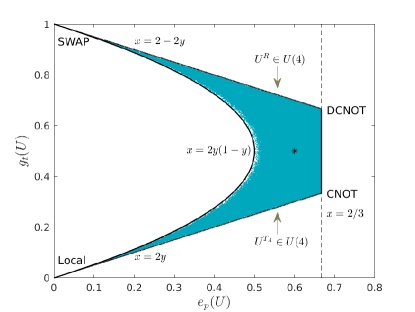
Figure 1: Set $K_{2}$ of all two-qubit gates projected into the plane entangling power, $x=e_{p}(U)$, versus gate-typicality, $y=g_{t}(U)$. Each point corresponds to a random unitary matrix from $U(4)$, while (*) represents the average over CUE. The boundaries $\partial K_{2}$ are identified in the text and in Fig. 2.

The upper bounds on $E(U)$ and $E(US)$ (equal to $3/4$) lead to the relations,

$$e_{p}+2g_{t}\leq 2\quad\text{and}\quad g_{t}\geq e_{p}/2,$$ (26)

which are the top and bottom lines in Fig. 1. The maximum value of $e_{p}=2/3$ is reached by the cnot gate and is an “optimal” gate in the terminology of Zanardi et al. (2000). The region is further restricted however and we will show below that the left boundary is given by the parabola $e_{p}=2g_{t}(1-g_{t})$. We further show in Sec. IV that this boundary in fact consists of gates of the form $S^{\alpha}$ with $0\leq\alpha\leq 1$, that are rational powers of the swap operator $S$.

The Weyl chamber and various gates

While the lines in Eq. (26) are bounds, we identify the gates that make these actual boundaries of the allowed set $K_{2}$ in the space $e_{p}$ vs $g_{t}$. It will be useful to work with the well known canonical form of a two-qubit unitary operator. Any two-qubit operator $U\in SU(4)$, upto left and right multiplication by local unitaries, can be expressed in terms of Euler angles $\{c_{1},c_{2},c_{3}\}\in[0,\pi]$ as Khaneja et al. (2001); Kraus and Cirac (2001); Zhang et al. (2003); Rezakhani (2004),

$$\begin{split}U=\exp\left[-i\left(\frac{c_{1}}{2}\sigma_{1}\otimes\sigma_{1}+\frac{c_{2}}{2}\sigma_{2}\otimes\sigma_{2}+\frac{c_{3}}{2}\sigma_{3}\otimes\sigma_{3}\right)\right],\end{split}$$ (27)

where $\{\sigma_{1},\sigma_{2},\sigma_{3}\}$ are the Pauli matrices. In the standard computational basis (the eigenbasis of $\sigma_{3}$), any bipartite unitary operator can thus be written as,

$$U=\left(\begin{array}[]{cccc}e^{\frac{-ic_{3}}{2}}c^{-}&0&0&-ie^{\frac{-ic_{3}}{2}}s^{-}\\ 0&e^{\frac{ic_{3}}{2}}c^{+}&-ie^{\frac{ic_{3}}{2}}s^{+}&0\\ 0&-ie^{\frac{ic_{3}}{2}}s^{+}&e^{\frac{ic_{3}}{2}}c^{+}&0\\ -ie^{\frac{-ic_{3}}{2}}s^{-}&0&0&e^{\frac{-ic_{3}}{2}}c^{-}\end{array}\right)$$

where,

$$c^{\pm}=\cos[(c_{1}\pm c_{2})/2];\qquad s^{\pm}=\sin[(c_{1}\pm c_{2})/2].$$ (28)

On imposing the constraint of local unitary equivalence, that is, if any two unitaries $U$ and $U^{\prime}=(u_{A_{1}}\otimes u_{B_{1}})U(u_{A_{2}}\otimes u_{B_{2}})$ related by local unitaries are represented by the same set of Euler angles, the range of values gets restricted to $|c_{3}|<c_{2}<c_{1}<\pi/2$. This region in the $\{c_{1},c_{2},c_{3}\}$ space containing the nonlocal two-qubit gates forms a tetrahedron known as the Weyl chamber Zhang et al. (2003).

In terms of the $\{c_{1},c_{2},c_{3}\}$ parametrization, it is known Zhang et al. (2003); Balakrishnan and Sankaranarayanan (2009) that one can define two quantities which are invariant under local unitary operations, namely,

$$\begin{split}G_{1}&=\cos^{2}c_{1}\cos^{2}c_{2}\cos^{2}c_{3}-\sin^{2}c_{1}\sin^{2}c_{2}\sin^{2}c_{3}\\ &+\frac{i}{4}\sin 2c_{1}\sin 2c_{2}\sin 2c_{3},\\ G_{2}&=\cos 2c_{1}+\cos 2c_{2}+\cos 2c_{3}.\end{split}$$ (29)

The operator entanglements $E(U)$ and $E(US)$ can be written in terms of local invariants $G_{1}$ and $G_{2}$, as follows Balakrishnan and Sankaranarayanan (2011):

$$\begin{split}E(U)&=1-\frac{1}{8}\left[3+2|G_{1}(U)|+G_{2}(U)\right],\\ E(US)&=1-\frac{1}{8}\left[3+2|G_{1}(U)|-G_{2}(U)\right].\end{split}$$ (30)

Consequently, the entangling power and gate-typicality of any two-qubit gate $U$ can be explicitly evaluated in terms of the angles $\{c_{1},c_{2},c_{3}\}$ and takes on an elegant and simple form as,

$$e_{p}(U) = \frac{2}{3}\left[\sin^{2}c_{1}\cos^{2}c_{2}+\sin^{2}c_{2}\cos^{2}c_{3}+\sin^{2}c_{3}\cos^{2}c_{1}\right],$$

$$g_{t}(U) = \frac{1}{3}\left[\sin^{2}c_{1}+\sin^{2}c_{2}+\sin^{2}c_{3}\right].$$ (31)

This leads to the following restriction on the allowed region in the $e_{p}-g_{t}$ plane for two-qubit gates.

Theorem III.1 (Boundary of two-qubit gates).

The entangling power $e_{p}(U)$ and gate-typicality $g_{t}(U)$ for any two-qubit unitary $U$ satisfy

$$e_{p}(U)\geq 2g_{t}(U)\left(1-g_{t}(U)\right).$$ (32)

Proof: Using Eq. (31), we see that $2g_{t}(U)(1-g_{t}(U))$ is of the form,

$$\!\!\!\!\!\!\!\!2g_{t}(U)(1-g_{t}(U))=\frac{2}{9}(x+y+z)(3-(x+y+z)),$$ (33)

where $x\equiv\sin^{2}c_{1}$, $y\equiv\sin^{2}c_{2}$, $z\equiv\sin^{2}c_{3}$ satisfy $0\leq x,y,z\leq 1$. Then, it is easy to see that,

$$(x+y+z)(3-(x+y+z))$$

$$= 3\left[x(1-y)+y(1-z)+z(1-x)\right]$$

$$+ \left(xy+yz+zx\right)-\left(x^{2}+y^{2}+z^{2}\right)$$

$$\leq 3\left[x(1-y)+y(1-z)+z(1-x)\right],$$

since $xy+yz+zx\leq x^{2}+y^{2}+z^{2}$, by Schwarz inequality. Using this in Eq. (33) above, we get,

$$2g_{t}(U)(1-g_{t}(U))$$ (34)

$$\leq \frac{2}{3}\left[x(1-y)+y(1-z)+z(1-x)\right]$$

$$= \frac{2}{3}\left[\sin^{2}c_{1}\cos^{2}c_{2}+\sin^{2}c_{2}\cos^{2}c_{3}+\sin^{2}c_{3}\cos^{2}c_{1}\right]$$

$$= e_{p}(U),$$

as desired. ∎

Gate $U$	$E(U)$	$E(US)$	$e_{p}(U)$	$g_{t}(U)$
Local-gate	0	$\frac{3}{4}$	0	0
$\sqrt{\textsc{cnot}}$	$\frac{1}{4}$	$\frac{3}{4}$	$\frac{1}{3}$	$\frac{1}{6}$
cnot, B-gate	$\frac{1}{2}$	$\frac{3}{4}$	$\frac{2}{3}$	$\frac{1}{3}$
dcnot	$\frac{3}{4}$	$\frac{1}{2}$	$\frac{2}{3}$	$\frac{2}{3}$
Fourier $F_{4}$	$\frac{3}{4}$	$\frac{1}{4}$	$\frac{1}{3}$	$\frac{5}{6}$
$\sqrt{\textsc{swap}}$	$\frac{9}{16}$	$\frac{9}{16}$	$\frac{1}{2}$	$\frac{1}{2}$
swap	$\frac{3}{4}$	$0$	$0$	$1$
Haar Average	$\frac{3}{5}$	$\frac{3}{5}$	$\frac{3}{5}$	$\frac{1}{2}$

Table 1: Nonlocal properties of selected two-qubit gates, $N=2$. Their location in the set $K_{2}$ is shown in Fig. 2.

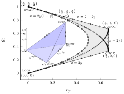
Figure 2: Boundaries of the set $K_{2}$ representing two-qubit gates in the plane $(e_{p},g_{t})$ are indicated by solid lines. Note distinguished gates identified in the plot. Inset shows edges of the tetrahedron in the parameter space $(c_{1},c_{2},c_{3})$ forming a half of the Weyl chamber Mandarino et al. (2018), which correspond to $\partial K_{2}$.

The inequality in Eq. (32) is tight, as the $S^{\alpha}$ family of gates with $0\leq\alpha\leq 1$ lie on the parabola $e_{p}(U)=2g_{t}(U)\left(1-g_{t}(U)\right)$. This is shown by an explicit calculation in Eq. (42), Sec. IV.

The cnot gate $C$ has the maximum entangling power of $2/3$, as expected. Furthermore, we show below that all members of the $CS^{\alpha}$ family, with $0\leq\alpha\leq 1$ have maximum entangling power of $2/3$ and form the rightmost vertical boundary in Figures 1 and 2. The gate $CS$ is the so-called double-cnot (dcnot) gate Collins et al. (2001). Note that,

$$U_{t}=\exp(itS)=\mathbb{1}\,\cos t+i\sin t\,S,$$ (35)

as $S^{2}=\mathbb{1}$, where, $\mathbb{1}$ denotes the identity operator. This is a route to defining fractional powers of $S$, as $\exp(i\pi S/2)=iS$ and therefore $(iS)^{t2/\pi}$ is same as $\exp(itS)$ and the overall phase of $i^{t2/\pi}$ makes no difference to any of the subsequent calculations. Therefore $U_{t}$ is essentially $S^{2t/\pi}$. The reshuffled matrix of $CS^{\alpha}$ is upto a constant phase given by,

$$(CS^{\alpha})^{R}=\cos(\pi\alpha/2)C^{R}+i\sin(\pi\alpha/2)(CS)^{R}.$$ (36)

The rearrangement of the cnot gate is non-unitary being $|00\rangle\langle 00|+|00\rangle\langle 11|+|11\rangle\langle 01|+|11\rangle\langle 10|$, while $(CS)^{R}$ is again a permutation given by $|00\rangle\langle 00|+|10\rangle\langle 11|+|01\rangle\langle 10|+|11\rangle\langle 01|$. A calculation then yields that

$$E(CS^{\alpha})=\frac{1}{8}(5-\cos(\pi\alpha))$$ (37)

Hence

$$e_{p}(CS^{\alpha})=\frac{1}{E(S)}\left[E(CS^{\alpha})+E(CS^{\alpha+1})-E(S)\right]=\frac{2}{3},$$ (38)

and $g_{t}(CS^{\alpha})=1/2-\cos(\pi\alpha)/6$ interpolating between $1/3$ and $2/3$.

Several other standard two qubit gates are identified and their operator entanglement and entangling powers are given in Table 1. We also identify gates in the Weyl chamber with different regions of the set $K_{2}$ contained in the plane $(e_{p},g_{t})$. In Figure 2, six edges of the tetrahedron forming a half of the chamber Mandarino et al. (2018) are shown. Four of these edges form four of the boundaries $\partial K_{2}$, the other two connect two of the extreme points symmetrically.

IV Beyond qubits and the entangling power of some quNit gates

Moving beyond qubits, we now study the entanglement landscape of bipartite unitary gates acting in a composite $N\times N$ quantum system. In this context, we investigate the Fourier gate and the fractional powers of the swap that form an important family of gates. We observe that for any $N\geq 2$, the fractional powers of swap lie on a parabola. The rightmost point is maximally entangling, at $e_{p}=1$ and $g_{t}=1/2$ and it is known that in all dimensions except $N=6$ (and $N=2$, which we have already dealt with) permutations exist which have these values. In the case $N=3$ explicit examples of permutations which have $e_{p}=1$ have been constructed Clarisse et al. (2005); Goyeneche et al. (2015).

The discrete Fourier transform, DFT, on the space $\mathcal{H}_{N}\otimes\mathcal{H}_{N}$ is given by the unitary gate $F_{N^{2}}$ of order $N^{2}$, with entries $F_{mn}=\frac{1}{N}\exp(2\pi imn/N^{2})$. This may be expressed in bipartite notation, as,

$$\langle k\alpha|F_{N^{2}}|j\beta\rangle=\frac{1}{N}e^{\frac{2\pi i}{N^{2}}[(k+\alpha N)(j+\beta N)]},$$ (39)

where $0\leq k,j,\alpha,\beta\leq N-1$. It is then straightforward to verify that the reshuffled matrix $F_{N^{2}}^{R}$ is also unitary Musz et al. (2013), and hence the operator entanglement is maximum possible: $E(F_{N^{2}})=1-1/N^{2}$. In this sense the Fourier gate in arbitrary dimensions is a dual-unitary, and a recent paper Gutkin et al. constructs dual kicked chains using the DFT, to study solvable Floquet many-body systems.

However, the partial transpose of the DFT is not unitary and hence the Fourier does not have maximal entangling power. Equivalently $E(F_{N^{2}}S)$ is not the maximal possible, instead a calculation yields

$$\begin{split}E(F_{N^{2}}S)=&1-\frac{1}{N^{4}}\left[N^{3}+2\sum_{k=1}^{N-1}k\frac{\sin^{2}\left(k\,\pi/N\right)}{\sin^{2}\left(\pi/N-k\,\pi/N^{2}\right)}\right]\\ &\approx 1-\frac{2}{\pi^{2}}\int_{0}^{1}\frac{x\sin^{2}(\pi x)}{(1-x)^{2}}\,dx\approx 0.344,\end{split}$$ (40)

where the approximation is valid for large $N$. Thus the operator entanglement of $F_{N^{2}}S$ and the entangling power of the Fourier gate $F_{N^{2}}$ tends to $\approx 0.344$, about one-third of the maximum possible.

As indicated in Eq. (35) above, the fractional powers of the swap $S$ up to phase factors are given by $U_{t}=\exp(itS)$. Since the reshuffled operator $S^{R}=S$, we get

$$U_{t}^{R} = \mathbb{1}^{R}\cos t+i\sin t\,S$$ (41)

$$= N|\Phi^{+}\rangle\langle\Phi^{+}|\cos t+i\sin t\,S,$$

where we have use the fact that the reshuffling of the identity is given by, $\mathbb{1}^{R}=N|\Phi^{+}\rangle\langle\Phi^{+}|$, with $|\Phi^{+}\rangle=\frac{1}{\sqrt{N}}\sum_{i=1}^{N}|ii\rangle$ being a maximally entangled state. Further, as $U_{t}\,S=S\,\cos t+i\mathbb{1}\sin t$, the following simple formulae follow for the fractional powers of the swap gate:

$$\begin{split}&E(e^{itS})=E(S)(1-\cos^{4}t),\;E(e^{itS}S)=E(S)(1-\sin^{4}t),\\ &e_{p}(e^{itS})=\frac{1}{2}\sin^{2}(2t),\;g_{t}(e^{itS})=\sin^{2}t.\end{split}$$ (42)

Thus, if $U_{t}$ is a fractional power of $S$ then $e_{p}(U_{t})=2g_{t}(U_{t})\left(1-g_{t}(U_{t})\right)$, in any dimension. We have already shown that this parabola is indeed the left-boundary of the set $K_{2}$ in the $(e_{p},g_{t})$ plane in the case of two-qubit gates.

To investigate the neighborhood of the parabola, we start with an operator of the form $S^{\alpha}$ and perturb it, while retaining the unitarity. There are many possible ways of doing such a perturbation, all of which yield equivalent results. For example one may deform $S^{\alpha}\rightarrow S^{\alpha}\exp(i\epsilon H)$ where $H$ is a random Hermitian matrix with unit variance and zero mean elements. Another approach is to use random matrices $V_{\epsilon}=U_{CUE}U_{d}(\epsilon)U_{CUE}^{\dagger}$ from the ensemble investigated in Poźniak et al. (1998) and defined by a Haar random unitary matrix $U_{CUE}$ and a diagonal matrix $U_{d}(\epsilon)$ with phases $\exp(i\epsilon\xi)$, where $\xi$ is uniform random number in $[-\pi,\pi)$. Powers of swap perturbed as $S^{\alpha}\rightarrow S^{\alpha}V_{\epsilon}$ result in values of $\{e_{p},g_{t}\}$ lying to the right of the parabola. Combined with the stationarity derived in Appendix (B), one may be tempted to conjecture that the parabola itself is a boundary. However, we have found an exception in a permutation in the qutrit case and can only conclude that typical perturbations of $S^{\alpha}$ result in a movement to the right of the parabola in the ($e_{p}$, $g_{t}$) plane.

Figure 3: (color online:) Unitary matrices $U\in U(9)$, representing two-qutrit gates, projected into the set $K_{3}$ in the plane $(e_{p},g_{t})$. Each color represents the neighbourhood of a particular gate, labeled with the same color. Upper side of the triangle, including Fourier matrix $F_{9}$, contains ‘dual unitaries’ for which $U^{R}$ is unitary, while the lower side includes these for which $U^{T_{A}}$ is unitary. Inset provides a magnified view of the region around the rightmost point representing the $2$-unitary gate $P_{9}$, with the CUE ‘cloud’, centered at $(1/2,4/5)$ (*), and shown in red and perturbations of different boundary gates in blue.

A similar study as in the case of $K_{2}$ was performed for unitary matrices belonging to the lower and the upper parts of the boundary of the set $K_{3}$. It is useful to distinguish certain unitary matrices, which correspond to points at $\partial K_{3}$. The controlled addition gate $C_{N}$ acting on a two-quNit system can be considered as a generalizations of the standard CNOT gate. In the case of $N=3$ such a gate reads,

$$\ C_{3}|i\rangle\otimes|j\rangle=|i\rangle\otimes|i\oplus j\rangle,\,\,i,j\in\mathbb{Z}_{3},$$ (43)

where $\oplus$ denotes addition modulo 3. This gate attains the maximal value of $E(C_{3}\,S)$ and lies in $K_{3}$ on its lower boundary, $y=2x$. It is seen that the perturbations have the tendency to quickly approach the CUE “cloud” in the manner of a jet.

In Fig. 3, the neighbourhood gates of several unitary quantum gates are generated for $N=3$ and the corresponding phase space plot is shown. The rightmost point of the set $K_{3}$ in the $(e_{p},g_{t})$ plane, denoted as $P_{9}$ in Fig. 3, corresponds to one of the permutations with $e_{p}=1$ defined in Clarisse et al. (2005); Goyeneche et al. (2015). The Fourier matrix $F_{9}$, attains the maximum value of $E(U)$, as $F_{9}^{R}$ is unitary, and lies on the upper boundary of $K_{3}$ formed by the line $x=2(1-y)$.

The upper boundary line contains maximally entangled unitary matrices, for which $U^{R}$ is also unitary. However, the partially transposed matrix $U^{T_{a}}$ is not unitary, with the exception of the matrices at the right corner of the triangle. Thus gates belonging to the upper boundary of $K_{N}$ are not $2$-unitary Goyeneche et al. (2015), but satisfy the weaker condition of being dual-unitaries Bertini et al. (2019b). Unitary gates for which $U^{T_{A}}$ is unitary, studied in Deschamps et al. (2016); Benoist and Nechita (2017) in context of quantum operations preserving some given matrix algebra, belong to the lower boundary line of $K_{3}$. Both lines cross at the right corner of the triangle, representing permutation $P_{9}$ and other $2$-unitary matrices, which maximize the entangling power.

It is interesting to observe that the set $K_{3}$ seems not to fill entire edge of the triangle close to the corner with $e_{p}=1$, as no dual unitaries in the vicinity of $P_{9}$ were found. This fact is borne out by numerical simulations that employ an algorithm to create an ensemble of dual ones Rather et al. (2019). The significance of the gap observed is to be fully explored, but the numerics suggest that the set of dual unitary matrices of size $N^{2}=9$ is not connected, in contrast to the two-qubit case, $N^{2}=4$. Since the dual unitary operators are related to four-party entanglement – see Appendix A – this implies some additional constraints on the entanglement in four-qutrit systems across different partitions and on possible spectra of two-partite density matrices obtained by partial trace of a pure state of size $N^{4}$.

Analysis of the non-local properties of any two-qubit gate becomes easier as the canonical form (27) is valid for any unitary matrix from $U(4)$. This form, related to a isomorphism in group theory between $SO(4)$ and $SU(2)\times SU(2)$ can not be generalized for two-qutrit gates. Therefore, our understanding of the set of bipartite gates acting on $N\times N$ systems in still not complete. The structure of the set $K_{N}$ obtained by a projection of $U(N^{2})$ into the plane $(e_{p},g_{t})$ is not entirely characterized even in the case $N=3$. Leaving these open problems for further studies we shall now move to a related problem, if a given bipartite unitary gate $U$ acts sequentially on a quantum system.

V Time evolution and multiple uses of the nonlocal operators

If $U$ is a bipartite quantum propagator, it is natural to consider a combination ${\mathcal{U}}=(u_{A}\otimes u_{B})U$ where the unitaries $u_{A},u_{B}$ are interpreted as “local dynamics” or single particle dynamics. We have motivated (see discussion around Eq. (4)) the study of its powers $\mathcal{U}^{n}$ as well as products $\mathcal{U}^{(n)}$ with different local operators in each term of the product.

The circuit in Fig 4 describes the time-evolution scenario considered here, for the case of qubit systems. Specifically, the circuit depicts the propagator $\mathcal{U}^{(n)}$ for $n=3$. The fixed nonlocal unitary $U\in U(4)$ is implemented via a combination of cnot gates and local rotations $R_{z}(t)$ and $R_{y}(t)$, following the prescription in Vatan and Williams (2004). The interlacing local qubit gates are denoted as $A_{i}$ and $A_{i}^{\prime}$, with $i=1,2$. We have omitted the initial set of local unitaries since they do not affect the entangling power. Note that the interlacing locals are different at each step, and hence labelled differently.

Observe that for a single time step the nonlocal content of $U$ is the same as that of ${\mathcal{U}}$, hence $e_{p}(U)=e_{p}({\mathcal{U}})$. Thus if the gate ${\mathcal{U}}$ is applied onto an unentangled initial state the local dynamics does not play any role in creation of quantum entanglement. However, the nonlocal content of multiple applications, either as ${\mathcal{U}}^{n}$ or $\mathcal{U}^{(n)}$, which represents discrete time evolution, is a different matter as the Schmidt coefficients of an operator in general change on taking powers. In this case the local dynamics can play a crucial role Jonnadula et al. (2017); Mandarino et al. (2018). For instance, in terms of entangling power

$$e_{p}({\mathcal{U}}^{2})=e_{p}\left[U(u_{A}\otimes u_{B})U\right]\neq e_{p}(U^{2}).$$ (44)

One of the aims of this paper is to analyze this difference and study the regime of large $n$. While we have presented related results earlier Jonnadula et al. (2017), this work contains an important generalization and a more elegant derivation that uses group theory. Note that we are interested in generic statements about average entanglement growth in time, a subject that already has a considerable literature and is still a topic of research.

@C=0.35em @R=1.2em & R_z(t_1) 1 A_1 R_z(t_1) 1 A’_1 R_z(t_1) 1
-1 R_y(t_2) R_y(t_3) -1 A_2 -1 R_y(t_2) R_y(t_3) -1 A’_2 -1 R_y(t_2) R_y(t_3) -1

Figure 4: Circuit representing the propagator $\mathcal{U}^{(3)}$ for a pair of qubits. The fixed nonlocal two-qubit gate $U$ is implemented via the sequence of cnots and rotation gates $R_{z}(t)$,$R_{y}(t)$. The gates $A_{i}$ and $A_{i}^{\prime}$ represent the interlacing local unitaries, which vary at each time step.

V.1 Thermalization of entangling power

The generalization allows for the subsystems $\mathcal{H}^{A}$ and $\mathcal{H}^{B}$ to have different dimensions $N$ and $M$, say $N\leq M$. The operator entanglement still follows from the Schmidt decomposition of $U$ as in Eq. (5) and is determined by the singular values of the reshuffled matrix $U^{R}$ of size $N^{2}\times M^{2}$. This gives the vector of local invariants $\lambda_{j}$, equal to eigenvalues of a positive matrix $U^{R}(U^{R})^{\dagger}$. The other set of invariants which in the symmetric case came from the Schmidt decomposition of $US$ in Eq. (9) now come from the singular values of the square matrix $U^{T_{A}}$ of size $NM\times NM$. The generalization of the expressions in (16) and (18) for entangling power Wang and Zanardi (2002) and gate-typicality, respectively, based on the reshuffled and partially transposed matrix $U$ is given by:

$$\begin{split}e_{p}(U)=&\frac{1}{M^{2}(N^{2}-1)}\left[NM(NM+1)-\right.\\ &\left.\mbox{tr}(U^{R}(U^{R})^{\dagger})^{2}-\mbox{tr}(U^{T_{A}}(U^{T_{A}})^{\dagger})^{2}\right],\\ g_{t}(U)=&\frac{1}{2NM(N+1)(M-1)}\left[N^{2}M^{2}-NM-\right.\\ &\left.\mbox{tr}(U^{R}(U^{R})^{\dagger})^{2}+\mbox{tr}(U^{T_{A}}(U^{T_{A}})^{\dagger})^{2}\right]\end{split}$$ (45)

Note that we use a normalization factor that implies that the maximal entangling power is equal to unity, which is attained when $\mbox{tr}(U^{R}(U^{R})^{\dagger})^{2}=M^{2}$ and $\mbox{tr}(U^{T_{A}}(U^{T_{A}})^{\dagger})^{2}=NM$. Hence our expression differs from the expression in Wang and Zanardi (2002) by a factor $\tilde{e}_{p}^{\text{max}}=\frac{M(N-1)}{N(M+1)}$, which is the unscaled maximum entangling power for a $N\times M$ bipartite system.

The generalization in Eq. (45) allows us to consider a situation where the bipartite interaction is non-zero but arbitrarily small and the second subsystem is considerably large, such as a thermal bath. In particular, we show in Theorem V.1 below, that

$$\begin{split}&\left\langle e_{p}\left[U(u_{A}\otimes u_{B})V\right]\right\rangle_{u_{A},u_{B}}\\ &=e_{p}(U)+e_{p}(V)-\,e_{p}(U)e_{p}(V)/\overline{e_{p}},\\ &\left\langle g_{t}\left[U(u_{A}\otimes u_{B})V\right]\right\rangle_{u_{A},u_{B}}\\ &=g_{t}(U)+g_{t}(V)-\,g_{t}(U)g_{t}(V)/\overline{g_{t}},\end{split}$$ (46)

Here $U$ and $V$ are any two unitary operators and the angular brackets indicate averaging over the local unitary operations with $u_{A,B}$ sampled uniformly (Haar measure). The quantities $\overline{e_{p}}$ and $\overline{g_{t}}$ are the Haar averages over the $MN$ dimensional space that generalize the expressions in Eq. (20), for subsystems of equal dimensions, to

$$\overline{e_{p}}=\frac{N(M^{2}-1)}{M(NM+1)},\,\ \ \overline{g_{t}}=\frac{(N-1)(M+1)}{2(NM-1)}.$$ (47)

The above discussion can be directly related to operator scrambling, which measures the spread of an initially localized operator Nahum et al. (2017); Chan et al. (2018); von Keyserlingk et al. (2018); Moudgalya et al. (2019). In the simplest bipartite setting, operator scrambling can be characterized by analyzing to what extent initially local operators become non-local. In analogy to the entangling power, wherein the action of operators on initially unentangled states is measured Zanardi et al. (2000); Zanardi (2001), we may consider time evolution of initial product operators in the Heisenberg picture of quantum mechanics. Such an evolution is obtained as a special case of Eq. (46), if $U=V^{\dagger}$. This may be interpreted as the average entangling power on conjugation of product operators with the bipartite operator $V$. As $e_{p}(V^{\dagger})=e_{p}(V)$, our results imply that

$$\left\langle e_{p}\left[V^{\dagger}(u_{A}\otimes u_{B})V\right]\right\rangle_{u_{A},u_{B}}=e_{p}(V)\left[2-\dfrac{e_{p}(V)}{\overline{e_{p}}}\right].$$ (48)

This provides a way to quantify the scrambling power of bipartite unitary operators. It would be interesting to generalize such a scrambling power for a multipartite setup, in analogy to the entangling power applied recently for several subsystems Linowski et al. (2020).

It might be surprising that simple relations (46) exists for $e_{p}$ and $g_{t}$, and this is due to the fact that they concern the average values. Similar relations hold for averaged operator entanglements $\left\langle E\left[U(u_{A}\otimes u_{B})V\right]\right\rangle_{u_{A},u_{B}}$ and $\left\langle E\left[U(u_{A}\otimes u_{B})V\,S\right]\right\rangle_{u_{A},u_{B}}$, but they mix among themselves in a less transparent way. Although the statements above concern averages over local unitaries, they provide some immediate insights. For instance, choosing $U$ and $V$ such that

$$e_{p}(U)+e_{p}(V)-\,e_{p}(U)e_{p}(V)/\overline{e_{p}}\;>\;e_{p}(UV),$$ (49)

we infer that there exist local unitaries which enhance the entangling power beyond a serial application of $V$ and $U$. Relations in Eq. (46) can be used to iterate, by inserting independent local operators between nonlocal operators. For example, one becomes

$$\begin{split}&\left\langle e_{p}\left[U(u_{A}\otimes u_{B})V(u^{\prime}_{A}\otimes u^{\prime}_{B})W\right]\right\rangle_{u_{A},u_{B},u^{\prime}_{A},u^{\prime}_{B}}\\ &=e_{p}(U)+e_{p}(V)+e_{p}(W)-[e_{p}(U)e_{p}(V)\\ &+e_{p}(V)e_{p}(W)+e_{p}(W)e_{p}(U)]/\overline{e_{p}}\\ &+e_{p}(U)e_{p}(V)e_{p}(W)/(\overline{e_{p}})^{2}.\end{split}$$ (50)

The above equation indicates a certain “decoupling” that is induced by local dynamics. It is necessary that the local operators at each product be independent, else the correlations prevent such an expression. However, previous work suggests Jonnadula et al. (2017) that they provide a good approximation, also in the case if the matrices $u_{A}$, $u_{A}^{\prime}$ and $u_{B}$, $u^{\prime}_{B}$ are pairwise identical, provided they are Haar - typical random unitaries.

We now formally state the result concerning the thermalization of the entangling power and gate typicality averaged over random local dynamics in the generalized setting of unequal dimensions of the subsystems. The final formulae remain the same as those displayed in Jonnadula et al. (2017), indicating a certain universality in them. However we present an alternate proof here, based on irreducible representations of the unitary group. Due to the technical nature of the proof, we present the details separately in Appendix C.

Theorem V.1.

Let $U$ and $V$ be bipartite unitary operators on $\mathcal{H}^{A}_{N}\otimes\mathcal{H}^{B}_{M}$ and $u_{A}$, $u_{B}$ be sampled from the groups $U(N)$ and $U(M)$ of unitary matrices according to their Haar measures. Then the following relation holds,

$$\begin{split}&\left\langle e_{p}\left[U(u_{A}\otimes u_{B})V\right]\right\rangle_{u_{A},u_{B}}\\ &=e_{p}(U)+e_{p}(V)-\,e_{p}(U)e_{p}(V)/\overline{e_{p}},\end{split}$$ (51)

where $\overline{e_{p}}=\langle e_{p}(W)\rangle_{W}$ denotes the mean entangling power averaged over random unitary matrices $W$ sampled according to the Haar measure on $U(NM)$.

Corollary V.1.1.

Let $U^{(n)}\equiv U\,(u_{A_{n-1}}\otimes u_{B_{n-1}})\,U\ldots(u_{A_{1}}\otimes u_{B_{1}})\,U$, where $u_{{A}_{j}}\in U(N)$ and $u_{B_{j}}\in U(M)$ are unitary matrices. Let $V=U^{(n-1)}$, so that $U^{(n)}=U(u_{A_{n-1}}\otimes u_{B_{n-1}})V$, then from the theorem above

$$\begin{split}\langle e_{p}{(U^{(n)})}\rangle_{\rm Loc}&=e_{p}(U)+\left[1-\frac{e_{p}(U)}{\overline{e_{p}}}\right]\langle e_{p}(U^{(n-1)})\rangle_{\rm Loc}\\ &=\overline{e_{p}}\left[1-\left(1-\frac{e_{p}(U)}{\overline{e_{p}}}\right)^{n}\right],\end{split}$$ (52)

where $\langle\ \cdot\ \rangle_{\rm Loc}$ denotes averaging over the set of local operators $u_{A_{n-1}},u_{B_{n-1}}\cdots u_{A_{1}},u_{B_{1}}$ generated independently according to the Haar measure.

Similarly it follows that

$$\langle g_{t}{(U^{(n)})}\rangle_{\rm Loc}={\bar{g}_{t}}\left[1-\left(1-\frac{g_{t}(U)}{\overline{g_{t}}}\right)^{n}\right],$$ (53)

where the average value ${\bar{g}_{t}}$ is provided in Eq. (47) and for $M=N$ reduces to $1/2$.

A proof of this result is indicated in Appendix C.

Eqs. (51) and (53) constitute our main results concerning thermalization of properties of quantum gates iterated sequentially in discrete time steps. For any bi-partite gate $U$ with arbitrary small, but positive entangling power, its repeated application with local unitaries sandwiched between consequtive time steps, leads to a generic gate with entangling power and gate typicality characteristic to the average over the ensemble of Haar random gates from $U(NM)$. The same is illustrated in Fig. 5 for qubits and qutrits in the $e_{p}-g_{t}$ plane. The evolution of $U^{n}$ and $\langle U^{(n)}\rangle_{\rm Loc}$ is shown for a particular (non-generic) choice of the initial unitary $U$, which selected from vicinity of a local gate, as $e_{p}(U)$ and $g_{t}(U)$ are sufficiently small. While $U^{n}$ explores the set $K_{N}$ in a “billiard” like dynamics Mandarino et al. (2018), $\langle U^{(n)}\rangle_{\rm Loc}$ converges exponentially to the CUE average.

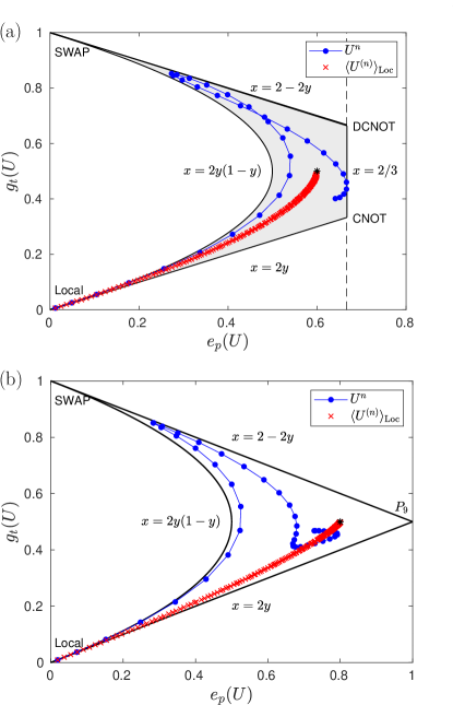
Figure 5: Exemplary dynamics in the set $K_{N}$ starting in a vicinity of a local gate for (a) $N=2$ and (b) $N=3$. The average value $\langle U^{(n)}\rangle_{\rm Loc}$, represented by red crosses ($\times$), saturates to the CUE average (*), while $U^{n}$ follows a billiard type dynamics Mandarino et al. (2018). Blue line joining the points in $U^{n}$ is added to guide the eye. At each time step, the average is taken over $10^{4}$ local random unitaries.

Our results involve averaging over different local operators at each time step and may be considered a foil for quantities such as $e_{p}[((u_{A}\otimes u_{B})U)^{n}]$ if $u_{A,B}$ are sufficiently random and have no special relationship with $U$. Thus while the above results may be applicable for non-autonomous Floquet systems, they are also of relevance to autonomous ones. In the case of a many-body spin chain, the effect of thermalization of the average entangling power to equilibrium has recently been reported Pal and Lakshminarayan (2018) for the symmetric case of $N=M$. The generalization presented here allows us to extend such studies of thermalization to the important case of different number of spins in each subsystem.

V.1.1 Example: random diagonal nonlocal operators

In Jonnadula et al. (2017) the entangling powers of $U^{n}$ and $U^{(n)}$ were evaluated for a few gates $U$, for the symmetric case $M=N$. Here we augment these results significantly, by numerically showing that for $N\neq M$, the thermalization of the entangling power to its average value $\overline{e_{p}}$ holds also in the case of a very small interaction between both subsystems. In particular, we analyze below the smallest interesting case of a qubit-qutrit system.

Consider a diagonal unitary matrix on $\mathcal{H}_{N}^{A}\otimes\mathcal{H}^{B}_{M}$ with entries

$$(U_{\epsilon})_{m\alpha;n\beta}=e^{2\pi i\epsilon\xi_{m\alpha}}\delta_{mn}\delta_{\alpha\beta},$$ (54)

where $\epsilon\in[0,1]$ and $\xi$ is chosen randomly and uniformly from $[-1/2,1/2)$. Such diagonal unitaries are used to model interactions in several deterministic Floquet operators Srivastava et al. (2016); Lakshminarayan et al. (2016); Tomsovic et al. (2018). While $\epsilon=0$ is evidently the case of zero interaction, $\epsilon=1$ represents the maximal interaction. As $\xi$ is a random variable, $(U_{\epsilon})_{m\alpha;n\beta}$ defines an ensemble of entangling gates. Their entangling power was studied in Lakshminarayan et al. (2014) for the case $\epsilon=1$, while for general $\epsilon$, it has been used in studies of spectral transitions and entanglement Srivastava et al. (2016); Lakshminarayan et al. (2016); Tomsovic et al. (2018).

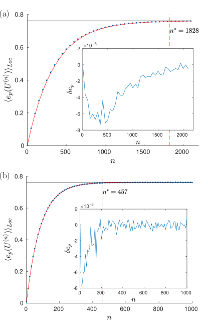
Figure 6: Saturation of entangling power $e_{p}$ for subsystems of size $N=2$ and $M=3$ as a function of discrete time $n$ for two values of the interaction parameter $\epsilon$, $\epsilon=0.025$ and 0.05 in (a) and (b), respectively. At each time step, the average is taken over $10^{4}$ local random unitaries. Solid curve represents Eq. (52), while the horizontal line denotes the Haar average $\overline{e_{p}}$ given by Eq. (47). Saturation time scales as $1/\epsilon^{2}$, see (58). The inset shows deviations from the theoretical values.

For a fixed realization of the global diagonal $U_{\epsilon}$, even if $\epsilon$ is very small, $\langle e_{p}(U_{\epsilon}^{(n)})\rangle_{\rm Loc}$ reaches the Haar average $\overline{e_{p}}$ due to interlacing of random local unitaries as illustrated in Fig. (6) in the case $MN=6$. For $e_{p}(U_{\epsilon})\ll 1$, Eq. (52) implies that

$$\langle e_{p}{(U_{\epsilon}^{(n)})}\rangle_{\rm Loc}\approx\overline{e_{p}}\,\left[1-\exp\left(-n\frac{e_{p}(U_{\epsilon})}{\overline{e_{p}}}\right)\right].$$ (55)

The saturation value reached is equal to the global average $\overline{e_{p}}$ which according to Eq. (47) reads $16/21\approx 0.762$ for $N=2$ and $M=3$. Smaller the interaction parameter, the longer it takes to thermalize and reach the asymptotic value. Deviations from the theoretical curve shown in the insets of Fig. (6) are of the order of $1/\sqrt{n_{loc}}$, where $n_{loc}$ denotes the number of realization of local gates over which the averaging is done. Hence the number of locals $n^{*}$ required to push $e_{p}(U_{\epsilon}^{(n)})$ to the Haar average depends on $\epsilon$ as $n^{*}\sim\overline{e_{p}}/e_{p}(U_{\epsilon})$.

The time of thermalization can be estimated for the case of local evolution given by the tensor product of diagonal random gates. For a diagonal unitary $U_{\epsilon}$ of size $NM\times NM$, the reshuffled matrix is of size $N^{2}\times M^{2}$ with $N(N-1)$ rows and $M(M-1)$ columns equal to zero. To compute $\mbox{tr}(U^{R}(U^{R})^{\dagger})^{2}$ in Eq. (45), it is thus sufficient to consider $\mbox{tr}(AA^{\dagger})^{2}$, where $A$ is obtained by reshaping the diagonal of $U_{\epsilon}$; $A_{jk}=e^{2\pi i\epsilon\xi_{\alpha}}$, $\alpha=(j-1)M+k$, $j=1,\dots,N$, $k=1,\dots,M$. Here $AA^{\dagger}$ is a Hermitian matrix of size $N$ and for $\epsilon$ small, $(AA^{\dagger})_{jj}=M$ and off-diagonal entries $(AA^{\dagger})_{jk}\approx M(1\pm i\epsilon)$, $j<k$. Thus,

$$\mbox{tr}(U_{\epsilon}^{R}(U_{\epsilon}^{R})^{\dagger})^{2}=\mbox{tr}(AA^{\dagger})^{2}\approx N^{2}M^{2}-N(N-1)M^{2}\epsilon^{2}$$ (56)

The partial transpose of a diagonal unitary remains unchanged, hence

$$\mbox{tr}(U_{\epsilon}^{T_{A}}(U_{\epsilon}^{T_{A}})^{\dagger})^{2}=NM.$$ (57)

Inserting Eq. (56) and Eq. (57) in Eq. (45) gives $e_{p}(U_{\epsilon})\approx N\epsilon^{2}/(N+1)$, and therefore

$$n^{*}\approx\frac{(N+1)(M^{2}-1)}{M(NM+1)}\;\frac{1}{\epsilon^{2}},$$ (58)

which for $N=2$, $M=3$ gives $n^{*}\approx 8\epsilon^{-2}/7$. For $\epsilon=0.025$ and $\epsilon=0.05$, the numerical values read $n^{*}\approx 1828$ and $n^{*}\approx 457$ respectively, as shown in Fig. (6).

For large dimensions $M$ and $N$, one may average additionally over the diagonal ensemble of the entangling gates themselves. It is possible to approximate such an ensemble averaged $\mbox{tr}(AA^{\dagger})^{2}$ by $N^{2}M^{2}\text{sinc}^{4}(\pi\epsilon)\approx(1-2\pi^{2}\epsilon^{2}/3)N^{2}M^{2}$, where sinc$(x)=\sin x/x$. Hence $e_{p}(U_{\epsilon})\approx 2\pi^{2}\epsilon^{2}/3$ and $n^{*}\sim 3\overline{e_{p}}/(2\pi^{2}\epsilon^{2})$, so that the saturation time scales as $1/\epsilon^{2}$.

Time evolution of quantum entanglement for initially separable states has been the subject of many studies Miller and Sarkar (1999); Bandyopadhyay and Lakshminarayan (2002); Fujisaki et al. (2003); Bandyopadhyay and Lakshminarayan (2004); Demkowicz-Dobrzański and Kuś (2004); Petitjean and Jacquod (2006), often in the context of weakly interacting highly chaotic systems. A recent study Pulikkottil et al. (2020) combining a recursive application of perturbation theory and the theory of random matrices indicates an exponential saturation of entanglement measures and is consistent with our findings. The approach advocated here is not perturbative and it is based on averaging of the entangling power over independent local operators at each time step. The rate at which the average $\langle e_{p}(U^{(n)})\rangle$ approaches the global RMT value $\bar{e}_{p}$ depends only on the entangling power of the nonlocal single-step operator $U$ and is hence fully interaction driven.

Note that the techniques applied in this work are not sensitive to the degree of chaos in the classical model consisting of two uncoupled systems. Thus analyzing the time evolution of averaged entangling power we are not in position to investigate the role of the Lyapunov exponent of the corresponding classical system, which was found essential Petitjean and Jacquod (2006) for the rate of growth of the average entanglement of quantum states initially localized in the phase-space. That the entangling power averages over all initial product states equally, implies that any special properties that arise for coherent initial states are washed out. However, further work is needed for clarifying the connections and differences between both approaches.

V.2 Thermalization of the spectra of reshuffled and partial transposed unitaries

We have analyzed above, how the local unitary invariants of entangling power and operator entanglement, and equivalently, the entropies of the density matrices in (21), thermalize in time to their asymptotic values. However, this only reflects a more detailed approach to equilibrium of the spectra of related operators. In particular, it is illuminating to analyze complex eigenvalues of non-unitary reshuffled and partially transposed matrices, $U^{(n)R}$ and $U^{(n)T_{A}}$, which allow us to infer, to what extent the analyzed gate approches properties characteristic to generic unitary matrices.

A large non-hermitian random matrix $G$ from the Ginibre ensemble, containing independent complex random Gaussian entries, displays spectrum covering uniformly the unit disk, according to the universal circular law of Girko Girko (1985); Bai (1997). If a random unitary matrix $U$ is large enough, the unitarity constraints become so weak that after reshuffling the matrix $U^{R}$ shows statistical properties close to these of the Ginibre ensemble Musz et al. (2013); Mandarino et al. (2018) - see also recent rigorous results Mingo et al. (2020). Thus the corresponding positive matrix, $U^{R}(U^{R})^{\dagger}$, display spectra in agreement with the the Marčenko-Pastur law Marčenko and Pastur (1967), $P_{MP}(x)=(2\pi)^{-1}\sqrt{(4-x)/x}$, derived to describe the spectral density of random Wishart matrices $GG^{\dagger}$.

Let $x_{i}$ denote eigenvalues of the density matrices $\rho_{R}(U^{(n)})$ or $\rho_{T}(U^{(n)})$ rescaled by the dimension $N^{2}$, which are equal to scaled squared singular values of $(U^{(n)})^{R}$ and $(U^{(n)})^{T_{A}}$ respectively. The thermalization of properties of the gate $U^{(n)}$ with the time $n$ will be reflected in the distribution $P(x)$, which for a large dimension $N$ converges to the distribution $P_{MP}(x)$. We will introduce local averaged purities of both auxiliary density matrices,

$$X_{n}=\langle\mbox{tr}[\rho_{R}^{2}(U^{(n)}]\rangle,\qquad Y_{n}=\langle\mbox{tr}[\rho_{T}^{2}(U^{(n)})]\rangle.$$ (59)

Then Marčenko-Pastur law implies that $X_{n}$ and $Y_{n}$ are of the order of $2/N^{2}$. A recursion relations for these quantities starting from $(X_{1},Y_{1})$ was derived in Jonnadula et al. (2017) for the symmetric case, $M=N$. We will now demonstrate thermalization in the spectra of density operators $\rho_{R}$ and $\rho_{T}$ for the model of the diagonal unitary ensemble and controlled unitaries.

V.2.1 Spectral properties for random diagonal nonlocal operators

Consider the special case of the model with nonlocal matrix $U$ being diagonal with random phases, as in Eq. (54). To focus on the effect of time evolution itself, we set the interaction strength to the maximal value, $\epsilon=1$, choose $N=M$, and denote the diagonal nonlocal matrix by $U=U_{d}$. Average purities of the density matrices defined in Eq. (59) for $n=1$ read,

$$\overline{X_{1}}=\frac{2N-1}{N^{2}}\quad\text{and}\quad\overline{Y_{1}}=\frac{1}{N^{2}}.$$ (60)

In this case there are no local operators and the averaging indicates only the average with respect to the random phases of the nonlocal operators $U_{d}$. The first one is easy to derive from the reshuffled operator, see Lakshminarayan et al. (2014) and since the partial transpose of a diagonal unitary matrix remains diagonal, $\rho_{T_{A}}(U_{d})=I_{N^{2}}/N^{2}$ hence, $Y_{1}=1/N^{2}$. Thus typical diagonal unitaries, even for $\epsilon=1$, are far from being thermalized, although their entangling power $e_{p}(U_{d})=(N-1)/(N+1)$ is large. This follows from Eq. (15), see also Lakshminarayan et al. (2014), in which a different normalization of the entangling power is used.

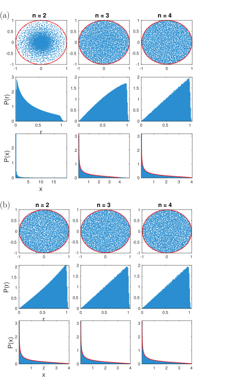
Figure 7: Spectral thermalization of $U^{(n)}$ for a random diagonal nonlocal unitary matrix $U_{d}$ of dimension $N^{2}$ with $N=50$. Distributions corresponding to (a) of reshuffled matrix $(U^{(n)})^{R}$ and (b) the partially transposed matrix $(U^{(n)})^{T_{A}}$, are shown for times $n=2,3$ and $4$. Top rows show the complex eigenvalues $z$, while middle rows show their radial density, $P(r)$ with $r=|z|$. The bottom rows show the distribution of scaled squared singular values of $(U^{(n)})^{R}$ and $(U^{(n)})^{T_{A}}$ respectively, which are compared with the Marčenko-Pastur distribution (solid curve).

For $n=2$ we consider an interlacing dynamics determined by random local unitary operators acting between two nonlocal operators, $U^{(2)}=U_{d}(u_{1}\otimes u_{2})U_{d}$, and obtain

$$\overline{X_{2}}=\frac{6}{N^{2}+1}\quad\text{and}\quad\overline{Y_{2}}=\frac{2(N^{4}+N^{2}+1)}{N^{4}(N+1)^{2}}.$$ (61)

Since $\overline{Y_{2}}\sim 2/N^{2}$, this quantity related to the partial transpose of $U_{d}$, is close to its asymptotic value already after two applications of typical nonlocal diagonal operators. On the other hand, the dual quantity $\overline{X_{2}}$ behaves as $6/N^{2}$, which indicates significant deviations from typicality.

These effects are visible in Fig. (7) in multiple ways. The eigenvalues of $(U_{d}^{(2)})^{R}$ are not distributed uniformly inside the unit disk, which is the case for the spectrum of $(U_{d}^{(2)})^{T_{A}}$. For the former operator there are several small eigenvalues which reflects the fact at $n=1$, the matrix $U_{d}^{R}$ is of rank $N$, rather than $N^{2}$. Even in the case of the partial transpose, there are visible deviations from linear structure of the radial distribution, which are not observed for $n\geq 3$. Although $\overline{X_{3}}\sim 2/N^{2}$, there exist deviations in the radial distribution, which thus serve as a sensitive indicator of thermalization. At $n=4$ the properties of the partial transpose and the reshuffled matrix are close to the matrices from the Ginibre ensemble of dimension $N^{2}$, and the singular values follow the Marčenko-Pastur law to a good approximation.

V.2.2 Spectral properties for controlled unitary operators

While the diagonal nonlocal operator lead to fast thermalization, for some other models this process occurs considerably slower. Consider a controlled unitary operator acting on a symmetric product space,

$$U=P_{A_{1}}\otimes\mathbb{1}_{B}+P_{A_{2}}\otimes u_{B}$$ (62)

where $P_{A_{i}}$ are orthogonal projectors such that $P_{A_{1}}+P_{A_{2}}=\mathbb{1}_{N}$, $P_{A_{i}}P_{A_{j}}=\delta_{ij}P_{A_{i}}$, and $u_{B}\in U(N)$. It is known Cohen and Yu (2013) that any two-qubit unitary gate of Schmidt rank two forms a controlled-unitary of this kind and it can be implemented with a maximally entangled state of two qubits and local operations and classical communication (LOCC). Thus this example may be considered the simplest entangling unitary. The reshuffled operator reads

$$U^{R}=|P_{A_{1}}^{R}\rangle\langle\mathbb{1}^{R}|+|P_{A_{2}}^{R}\rangle\langle u_{B}^{*R}|,$$ (63)

where $|M\rangle$ reshapes or vectorizes the operator with elements $M_{ij}=\langle i|M|j\rangle$ into a column vector with entries $M_{ij}$. Noting that $\langle M_{1}|M_{2}\rangle=\mbox{tr}(M_{1}^{\dagger}M_{2})$, we get

$$\begin{split}\rho_{R}=&\frac{1}{N^{2}}U^{R}U^{R\dagger}=\frac{1}{N^{2}}\left[N(|P_{A_{1}}^{R}\rangle\langle P_{A_{1}}^{R}|+|P_{A_{2}}^{R}\rangle\langle P_{A_{2}}^{R}|)+\right.\\ &\left.\mbox{tr}(u_{B})^{*}|P_{A_{1}}^{R}\rangle\langle P_{A_{2}}^{R}|+\mbox{tr}(u_{B})|P_{A_{2}}^{R}\rangle\langle P_{A_{1}}^{R}|\right],\end{split}$$ (64)

which is only a rank-2 operator. In contrast, as $(u_{A}\otimes u_{B})^{T_{A}}=u_{A}^{T}\otimes u_{B}$ and as transposes of projectors remain projectors, $U^{T_{A}}$ is also unitary and hence $\rho_{T}=\mathbb{1}_{N^{2}}/N^{2}$, a maximally mixed state. These observations immediately imply that

$$X_{1}=\frac{1}{2}+\frac{1}{2N^{2}}|\mbox{tr}(u_{B})|^{2},\quad\text{and}\quad Y_{1}=\frac{1}{N^{2}}.$$ (65)

Figure 8: As in Fig. 7 for $U$ selected as a controlled unitary gate. Third column plotted for $n=14$ and $n=10$ illustrates longer time required in this case to reach typicality.

Taking Haar random unitary matrices $u_{B}$ of size $N$ one defines an ensemble of controlled-unitary gates of order $N^{2}$, for which we evaluate the average purities of the associated density matrices $\rho_{R}(U^{(n)})$ and $\rho_{T}(U^{(n)})$. Form factor averaged over CUE matrices of size $N$ reads: $\overline{|\mbox{tr}(u_{B}^{n})|^{2}}=n$ if $n\leq N$ and $N$ for $n\geq N$ – see Haake et al. (1996). Denoting this additional averaging by an overbar one obtains $\overline{X_{1}}\sim 1/2$ and $\overline{Y_{1}}=1/N^{2}$. Using the recursion relation from Jonnadula et al. (2017) and the CUE form factors quoted above for $n=2$ we arrive at,

$$\begin{split}\overline{X_{2}}&=\frac{N^{6}+2N^{4}-6N^{2}+4}{4N^{2}(N^{2}-1)^{2}},\\ \overline{Y_{2}}&=\frac{5N^{4}-10N^{2}+6}{4N^{2}(N^{2}-1)^{2}}.\end{split}$$ (66)

The other details of the unitary gate $u^{B}$, are relevant to higher orders. It is also clear that the sequence $Y_{n}$ approaches the typical behavior earlier than the $X_{n}$. For instance, at $n=2$ we have $\overline{X_{2}}\sim 1/4$, while $\overline{Y_{2}}\sim\frac{5}{4N^{2}}$. In general, $\overline{X_{n}}\sim\frac{1}{2^{n}}$, indicating that it takes a time $n^{*}\sim 4\log_{2}N$ for the operators to thermalize, such that the average operator entanglement is comparable to the average over $U(N^{2})$. Numerical data obtained for a typical controlled unitary gate presented in Figure 8 show that in this case the thermalization time is longer in comparison to random diagonal gates. Even at $n=12$ one can see substantial deviations from the Girko circular law for the eigenvalues of the reshuffled matrix, while at $n=14$ the data become well described by the universal Marčenko-Pastur distribution. Spectral properties of the partially transposed matrix also reach typical behaviour around $n\sim 10$. These time scales are consistent with the $~{}\log_{2}N$ scale and the thermalization of the controlled-unitary gates occurs more slowly, but surely.

VI Summary and outlook

In this work we have investigated nonlocal properties of bipartite quantum gates acting on an $N\times M$ system. Representing them in the plane spanned by entangling power $e_{p}$ and gate typicality $g_{t}$, we have analyzed the boundary of the allowed set $K_{2}$, which in turn enabled us to identify gates that correspond to critical points of the boundary and are distinguished by some particular properties. Making use of the Cartan decomposition and the canonical form of a two-qubit gate Khaneja et al. (2001); Kraus and Cirac (2001) we have described the boundaries analytically, as they correspond to the edges and diagonals of the Weyl chamber.

As the Cartan decomposition is not effective for unitary matrices of order nine, in the case of two-qutrit gates such an approach does not work, hence only some parts of the boundary of the set $K_{3}$ are known exactly. For instance, the structure of $K_{3}$ is still unknown in the vicinity of the right most point representing optimal gates, for which entangling power admits its maximal value, $e_{p}=1$, and corresponds to maximally entangled states of a four–qutrit system. It is worth emphasizing that while such a gate does not exist for $N=2$ Higuchi and Sudbery (2000a), the case of $N=6$ still remains open Horodecki et al. (2020).

A key issue addressed in this paper concerns nonlocal properties of a bipartite unitary gate applied sequentially. Although local unitary operations performed after a single usage of a nonlocal gate cannot change its entangling power, they do play a crucial role if the gate analyzed is performed several times. Our result shows that an arbitrary small, but positive, entangling power of a nonlocal gate $U_{AB}$ is sufficient to assure that the gate $U^{\prime}_{AB}=U_{AB}V_{\rm loc}$ applied $n$ times will reach the entangling power typical to random unitary matrices exponentially fast. Here $V_{\rm loc}=u_{A}\otimes u_{B}$ denotes a random local unitary, which is drawn independently at each time step. This statement illustrates the thermalization of non-local properties of bipartite gates with the interaction time and sheds more light into the properties of quantized chaotic dynamics, in which nonlocal kicks coupling both subsystems are interlaced by chaotic local evolution Haake et al. (2018).

While the entangling power of a bipartite gate $U_{AB}$ determines the entangling power of time-evolutions augmented with local operators, it is interesting to note that it can possibly determine the complexity of the corresponding many-body systems built out of them in various architectures. As a concrete example, a product of $\otimes^{L}U_{AB}$ on a one-dimensional lattice of $2L$ sites and its translation by one-site was studied recently in terms of its correlation functions Bertini et al. (2020). It is not hard to infer from their results that the case when $U_{AB}$ has maximal entangling power allowed by the dimensions, corresponds to the case of a maximally chaotic many-body system. It is interesting to observe that qubits do not satisfy this condition, while this is the case for qutrits Clarisse et al. (2005). Thus we believe that our study is also relevant to a large body of recent work around understanding of quantum chaos for many-body systems.

Appendix A Bipartite unitary gates and four-party entangled pure states

The bijection between states on ${\cal H}^{(1)}\otimes{\cal H}^{(2)}$ and operators on ${\cal H}^{(1)}\cong{\cal H}^{(2)}$ is known in the physics litarature under the name Choi-Jamiołkowski isomorphism, which relates the set of pure states of a bipartite system and the set of operations acting on a simple system Bengtsson and Życzkowski (2007). Any normalized bipartite pure state $|\psi\rangle=\sum_{ij=1}^{N}x_{ij}|ij\rangle$ can be written as $(X\otimes\mathbb{1})|\phi^{+}\rangle$, where $|\phi^{+}\rangle=\sum_{j=1}^{N}|jj\rangle/\sqrt{N}$ is the maximally entangled state and $\langle i|X|j\rangle=\,\sqrt{N}x_{ij}$. Note that a state $|\psi\rangle$ is maximally entangled, if and only if the matrix $X$ is unitary, as then its partial trace is maximally mixed, $\rho_{A}={\rm tr}_{B}|\psi\rangle\langle\psi|=XX^{\dagger}/N=\mathbb{1}/N$. It is often convenient to make use of this relation between the set $U(N)/U(1)$ of unitary quantum gates of order $N$ and the set of maximally entangled states in $N\times N$ system Bengtsson and Życzkowski (2007).

The same relation can also be used in a more general set-up, if the system ${\cal H}^{(1)}$ is composite and describes two subsystems of sizes $N$ and $M\geq N$, denoted $A$ and $B$ respectively. The system ${\cal H}^{(2)}$ of the same size $NM$ is also composite and contains two subsystems $C$ and $D$ of dimensions $N$ and $M$ respectively. The matrix $X/\sqrt{NM}$ with elements $x_{i\alpha,k\beta}$ describes now a $4$-party pure state $|\psi_{ABCD}\rangle=\sum_{ij}^{N}\sum_{\alpha\beta}^{M}x_{i\alpha,k\beta}|i\alpha k\beta\rangle$, and can be considered as a four-index tensor or a $NM\times NM$ matrix with composite indices.

Any bi-partite matrix $X$ acting on subsystems $AB$, thus defines a four-partite pure state,

$$|\psi_{ABCD}\rangle=(X_{AB}\otimes\mathbb{1}_{CD})|\phi_{AC}^{+}\rangle\otimes|\phi_{BD}^{+}\rangle.$$ (67)

Note that the above formula does not factorize, as the symbol $\otimes$ denotes tensor products acting with respect to different partitions. If the bipartite matrix acting on the subsystems $AB$ is unitary, $X=U$, then the corresponding four party state $|\psi_{ABCD}\rangle$ is maximally entangled with respect to the partition $AB|CD$, so all the components of the corresponding Schmidt vector of length $NM$, eigenvalues of $\rho_{AB}={\rm tr}_{CD}|\psi_{ABCD}\rangle\langle\psi_{ABCD}|=UU^{\dagger}/NM$, are equal to $1/NM$. Unitarity condition, $UU^{\dagger}=\mathbb{1}$, implies then the maximal entanglement of the state $|\psi_{ABCD}\rangle$ with respect to the splitting $AB|CD$.

On the other hand, one can investigate whether this state is entangled with respect to two other possible partitions, $AC|BD$ and $AD|BC$. To this end one studies the partially reduced states $\rho_{AC}={\rm tr}_{BD}|\psi_{ABCD}\rangle\langle\psi_{ABCD}|$ with spectrum $\lambda_{i}$, with $1\leq i\leq N^{2}$ and $\rho_{AD}={\rm tr}_{BC}|\psi_{ABCD}\rangle\langle\psi_{ABCD}|$ with spectrum $\mu_{j}$ with $1\leq j\leq NM$.

For any four-index matrix $X_{ij,\alpha\beta}$ of size $NM$ it will be convenient to use the following operations on its entries Bengtsson and Życzkowski (2007): the partial transpose, $X^{T_{A}}$, where $X_{i\beta,j\alpha}^{T_{A}}=X_{i\alpha,j\beta}$, is also an $NM\times NM$ matrix, and the reshuffling, $X^{R}$, where $X_{ij,\alpha\beta}^{R}=X_{i\alpha,j\beta}$ is an $N^{2}\times M^{2}$ dimensional array. The first one, $T_{A}$, represents transposition on the first subsystem only and preservs hermiticity of $X$. The reshuffling $R$, corresponds to reshaping each block of a matrix into a vector, does not preserve unitarity nor hermiticity.

It is easy to check Życzkowski and Bengtsson (2004) that the vector $\lambda$, equal to the spectrum of the positive matrix

$$\rho_{R}(U)\equiv\rho_{AC}=U^{R}(U^{R})^{\dagger}/(NM),$$ (68)

coincides with the vector defining the operator Schmidt decomposition of the scaled matrix $U$. Correspondingly, the vector $\mu$, forming the spectrum of

$$\rho_{T_{A}}(U)\equiv\rho_{AD}=U^{T_{A}}(U^{T_{A}})^{\dagger}/(NM),$$ (69)

appears in the Schmidt decomposition of the operator $U$ composed with the swap $S$ for the symmetric case.

The reduced state of the subsystems $AC$ is maximally mixed if $\rho_{AC}=\mathbb{1}_{N^{2}}/N^{2}$ and corresponds to the maximum entanglement in the $AC|BD$ split. This in turn happens when the rearrangement $U^{R}$ satisfies $U^{R}(U^{R})^{\dagger}=\mathbb{1}_{N^{2}}/(MN)$, where $\mathbb{1}_{N^{2}}$ is the identity matrix of dimension $N^{2}$. In other words, for the symmetric case, $N=M$, if $U^{R}$ is also unitary, then $\rho_{R}(U)$ is maximally mixed and the subsystem $AC$ is maximally mixed with $BD$. Hence the linear entanglement entropy $1-\mbox{tr}_{AC}\rho_{AC}^{2}$, based on the reshuffling of $U$ can serve as a measure of the entanglement in the four-party state in Eq. (67) with respect to the partition $AC|BD$.

The state $|\psi_{ABCD}\rangle$ is maximally entangled with respect to the third splitting $AD|BC$ if the Schmidt vector is flat, $\mu_{j}=1/MN$ for $j=1,\dots,NM$, so that the matrix $X^{T_{A}}$ is unitary. Entanglement for this partition can be thus characterized by the twin quantity $1-\mbox{tr}_{AC}\rho_{AD}^{2}$.

Analyzing a bipartite unitary gate $U$, described by a four-index matrix $U_{a,b}=X_{i\alpha,j\beta}$, it is convenient to introduce the notion of multiunitarity Goyeneche et al. (2015). For the symmetric case ($N=M$), a matrix $X$ of size $N^{2}$, wrtitten in the four-index notation, is called $2$–unitary, if the following three conditions are satisfied

$${\rm i)}\ \ X\in U(N^{2})\Leftrightarrow\sum_{ij}X_{ij,\alpha\beta}{\bar{X}_{ij,\alpha^{\prime}\beta^{\prime}}}=\delta_{\alpha,\alpha^{\prime}}\delta_{\beta,\beta^{\prime}},$$

$${\rm ii)}\ \ X^{R}\in U(N^{2})\Leftrightarrow\sum_{i,\alpha}X_{ij,\alpha\beta}{\bar{X}_{ij^{\prime},\alpha\beta^{\prime}}}=\delta_{j,j^{\prime}}\delta_{\beta,\beta^{\prime}},$$

$${\rm iii)}\ \ X^{T_{A}}\in U(N^{2})\Leftrightarrow\sum_{i,\beta}X_{ij,\alpha\beta}{\bar{X}_{ij^{\prime},\alpha^{\prime}\beta}}=\delta_{j,j^{\prime}}\delta_{\alpha,\alpha^{\prime}},$$

so apart of $U$, also two other matrices with interchanged entries, $U^{T_{A}}$ and $U^{R}$, are unitary. The corresponding four-index tensor $X_{i\alpha,j\beta}$ of size $N$, is called perfect, if for any choice of two indices out of four, the matrix of size $N^{2}$ obtained by restructuring the four-index tensor into a matrix is unitary Pastawski et al. (2015). By construction, any $2$-unitary matrix $U$ of order $N^{2}$ provides an example of a matrix which maximizes the entangling power, $e_{p}(U)=1$, as both linear entanglement entropies $E(U)$ and $E(US)$ are maximal. Thus the corresponding four-party state (67) is maximally entangled with respect to all three possible partitions. Such states are called two-uniform Scott (2004) or absolutely maximally entangled (AME) Helwig et al. (2012).

Interestingly, such states do not exist in a four-qubit system Higuchi and Sudbery (2000a), as the total size of the Hilbert space is too small to find a state satisfying all necessary constraints. This is equivalent to the known fact Zanardi et al. (2000); Clarisse et al. (2005) that there is no unitary matrix of size $N^{2}=4$, for which the maximal value $e_{p}=1$ of the entangling power is achieved, which is consistent with the structure of the set $K_{2}$ plotted in Fig. 1. In the complementary notation, there are no $2$-unitary matrices of order four Goyeneche et al. (2015). On the other hand AME states exists for larger systems consisting of four qutrits, which is equivalent to the statement that there exists a $2$-unitary matrix of size $N^{2}=9$, which maximizes the entangling power $e_{p}$ Clarisse et al. (2005). For any $N=3,4,5$ and $N\geq 7$ there exist permutations matrices of size $N^{2}$ which are $2$-unitary, and hence maximize the entangling power Clarisse et al. (2005) and also correspond to AME states of four systems with $N$ levels each. For $N=6$, the non-existence of any $2$-unitary permutation matrix of order $36$ is directly related to the famous problem of $36$ officers by Euler and follows from the non-existence of two mutually orthogonal Latin Squares of size six. The more general question as to whether there exists a $2$-unitary matrix of size $N^{2}=36$ (not necessarily a permutation) remains open Horodecki et al. (2020).

Two unitarity of a bipartite gate $U$, corresponds to a two-uniform pure state of four parties, maximally entangled with respect to all three partitions. Sometimes it is interesting to relax one requirement and analyze pure state $|\psi_{ABCD}\rangle$ for which only two partial traces out of three are maximally mixed. This weaker condition corresponds to a unitary matrix $U$ of size $N^{2}$ such that additionally $U^{T_{A}}$ or $U^{R}$ is unitary. The class of unitary matrices such that the partial transposition $U^{T_{A}}$ remains unitary was studied in context of quantum operations preserving some given matrix algebra, and a method to generate them numerically based on a kind of the Sinkhorn algorithm was proposed Deschamps et al. (2016); Benoist and Nechita (2017). Such a technique based on alternating projections on manifolds converges Lewis and Malick (2008), if we wish to assure that two unitarity conditions are satisfied, so that two partial traces of the corresponding four-party state are fixed Duan et al. , but it will usually become less effective if three conditions (A) need to be fulfilled simultaneously.

The observations made in this Appendix for the symmetric case, $M=N$, can be summarized as follows.

Proposition 1.

For any unitary operator $U$ acting on a bipartite space $\mathcal{H}_{N}^{A}\otimes\mathcal{H}_{N}^{B}$, the following are equivalent.

• The unitary $U\in U(N^{2})$ attains the global maximum of entangling power, that is, $e_{p}(U)=1$, as both linear entanglement entropies $E(U)$ and $E(US)$ are maximal.

• The bipartite unitary matrix $U$ is $2$-unitary. In other words both the transformed matrices $U^{R}$ and $U^{T_{A}}$ remain unitary.

• If $U_{AB}=U$, the pure state

  $$|\psi_{ABCD}\rangle=(U_{AB}\otimes\mathbb{1}_{CD})|\phi_{AC}^{+}\rangle\otimes|\phi_{BD}^{+}\rangle$$

  defined in Eq. (67) is maximally entangled with respect to all possible bipartitions and thus forms an absolutely maximally entangled state of four quNits.

• The corresponding four-index tensor $u_{i\alpha,k\beta}$ whose elements describe the four-partite state

  $$|\psi_{ABCD}\rangle=\sum_{i,j=1}^{N}\sum_{\alpha,\beta=1}^{N}u_{i\alpha,j\beta}|i\alpha j\beta\rangle$$

  is perfect.

Appendix B The stationarity of the parabola of powers of swap

Lemma B.1.

Define $f(u)\equiv e_{p}(u)-2g_{t}(u)\bigl{(}1-g_{t}(u)\bigr{)}$, where $e_{p}(u)$ and $g_{t}(u)$ are respectively the entangling power and gate typicality of a bipartite unitary $u$. The function $f(u)$ is extremised whenever $u=U_{t}=e^{itS}$ is a fractional power of the swap operator.

Proof.

Operators close to arbitrary fractional powers of swap $U_{t}$, with $0<\epsilon\ll 1$ are

$$U_{t,\epsilon}=\exp(itS+i\epsilon H)\approx\exp(itS)\left(\mathbb{1}+i\epsilon H\right),$$ (71)

where $H$ is a Hermitian operator. We may require without loss of generality that $H$ is traceless, that is $\mbox{tr}H=0$, as the overall phase will make no difference to calculations. We may also assume that $H$ is orthogonal to $S$, that is $\mbox{tr}(HS)=\mbox{tr}(SH)=0$, as any overlap with $S$ will be equivalent to only shifting $t$ to a new value. The difference $\delta U_{t}=U_{t,\epsilon}-U_{t}$ is given by

$$\delta U_{t}=i\epsilon\left(\cos t\,H+i\sin t\,SH\right).$$ (72)

We will show that $\delta E(U_{t})=0$ and $\delta E(U_{t}S)=0$, thus under such perturbations $\delta e_{p}(U_{t})=0$ and $\delta g_{t}(U_{t})=0$ and finally $\delta f(u=U_{t})=0$.

From Eq. (22) it follows that

$$\delta E(U)=-\frac{4}{N^{2}}\,\text{Re}\,\mbox{tr}\left(\delta U^{R}U^{R\,\dagger}U^{R}U^{R\,\dagger}\right).$$ (73)

From the linearity of the reshuffling operation, $\delta U_{t}^{R}=(U_{t,\epsilon})^{R}-U_{t}^{R}=(\delta U_{t})^{R}$. From this and Eq. (72) we get

$$\delta U_{t}^{R}=(\delta U_{t})^{R}=i\epsilon\left(\cos tH^{R}+i\sin t(SH)^{R}\right).$$ (74)

To show that $\mbox{tr}\left(\delta U_{t}^{R}U_{t}^{R\,\dagger}U_{t}^{R}U_{t}^{R\,\dagger}\right)=0$, we note that it involves $\mbox{tr}(H^{R}\mathbb{1}_{R})$, $\mbox{tr}(H^{R}S)$, $\mbox{tr}((SH)^{R}\mathbb{1}_{R})$ and $\mbox{tr}((SH)^{R}S)$. It is straightforward to verify that when $H$ is orthogonal to $S$ and is traceless, all of these vanish. In a similar way it is easy to show also that $\mbox{tr}\left(\delta U_{t}^{T_{A}}U_{t}^{T_{A}\,\dagger}U_{t}^{T}U_{t}^{T_{A}\,\dagger}\right)=0$. Thus $\delta f(u=U_{t})=0$ when $u=U_{t}$ is a power of the swap $S$, except when $\delta u$ is along $S$. In the latter case, $f(u)=0$ strictly and there is no variation of $f$, establishing that $f(u)$ is indeed an extremum if $u=e^{itS}$ is a fractional power of the swap. ∎

Appendix C Proof of the theorem concerning average entangling power $e_{p}[\mathcal{U}^{(n)}]$

Theorem C.1.

Let $U$ and $V$ be unitary operators on $\mathcal{H}^{A}_{N}\otimes\mathcal{H}^{B}_{M}$ and $u_{A}$, $u_{B}$ be sampled from the groups $U(N)$ and $U(M)$ of unitary matrices according to their Haar measures, then

$$\begin{split}&\left\langle e_{p}\left[U(u_{A}\otimes u_{B})V\right]\right\rangle_{u_{A},u_{B}}\\ &=e_{p}(U)+e_{p}(V)-\,e_{p}(U)e_{p}(V)/\overline{e_{p}},\end{split}$$ (75)

where the average entnagling power reads $\overline{e_{p}}=\langle e_{p}(W)\rangle_{W}$, and $W$ is sampled according to the Haar measure on the unitary group $U(NM)$.

Proof.

Consider an extended Hilbert space $\mathcal{H}_{N}^{A}\otimes\mathcal{H}_{M}^{B}\otimes\mathcal{H}^{C}_{A}\otimes\mathcal{H}^{D}_{M}$ where $\mathcal{H}^{C}_{N}$ are $\mathcal{H}^{D}_{M}$ are copies of $\mathcal{H}^{A}_{N}$ and $\mathcal{H}^{B}_{M}$. Using the identity $\mbox{tr}(\rho_{A}\otimes\rho_{C}S_{AC})=\mbox{tr}(\rho_{A}^{2})$ where $\rho_{C}$ is a copy of $\rho_{A}$ and $S_{AC}$ is the swap operator, the entangling power of $U$ acting on $\mathcal{H}^{A}_{N}\otimes\mathcal{H}^{B}_{M}$ was written in (Zanardi et al., 2000) as

$$\begin{split}e_{p}(U)&=\frac{2}{\tilde{e}_{p}^{\text{max}}}\,\mbox{tr}(U^{\otimes 2}\Omega^{++}_{p}{U^{\dagger}}^{\otimes 2}\Pi^{-}_{AC}).\end{split}$$ (76)

Here $\Pi^{-}_{AC}=2^{-1}(\mathbb{1}-S_{AC})$ is the projector over the anti-symmetric subspace of $\mathcal{H}^{A}_{N}\otimes\mathcal{H}^{C}_{N}$, and $\Omega^{++}_{p}=\omega_{AC}^{+}\otimes\omega_{BD}^{+}$ and $\omega_{AC}^{+}=\int d\mu(\psi_{A})(|\psi_{A}\rangle\langle\psi_{A}|\otimes|\psi_{A}\rangle\langle\psi_{A}|)$, while $\omega_{BC}^{+}$ is an identical operator. When $d\mu(\psi_{A})$ is the Haar measure on states in $\mathcal{H}^{A}_{N}$, recognizing that $\omega^{+}_{AC}$ has support only on the symmetric subspace, group theoretic arguments involving Schur’s lemma were used in (Zanardi et al., 2000) to show that $\Omega^{++}_{p}=4C_{A}C_{B}\Pi^{+}_{AC}\Pi^{+}_{BD}$. Here $C_{A}^{-1}=N(N+1)$, $C_{B}^{-1}=M(M+1)$, $\Pi^{+}_{AC}=2^{-1}(\mathbb{1}+S_{AC})$ is the projector over the symmetric subspace of $\mathcal{H}^{A}_{N}\otimes\mathcal{H}^{C}_{N}$, while $\Pi^{+}_{BD}$ is a similar projector on $\mathcal{H}^{B}_{M}\otimes\mathcal{H}^{D}_{M}$.

This forms a convenient starting point for us, as the local unitary averaged entangling power is

$$\left\langle e_{p}(U(u_{A}\otimes u_{B})V)\right\rangle_{u_{A},u_{B}}=\frac{2}{\tilde{e}_{p}^{\text{max}}}\,\mbox{tr}(U^{\otimes 2}\left\langle Q\right\rangle{U^{\dagger}}^{\otimes 2}\Pi^{-}_{AC})$$ (77)

where $Q=V\otimes V\Omega^{++}_{p}V^{\dagger}\otimes V^{\dagger}$, and

$$\begin{split}\left\langle Q\right\rangle=&\int d\mu(u_{A})\,d\mu(u_{B})(u_{A}\otimes u_{B})^{\otimes 2}\,\\ &V^{\otimes 2}\,\Omega^{++}_{p}\,{V^{\dagger}}^{\otimes 2}\,(u_{A}^{\dagger}\otimes u_{B}^{\dagger})^{\otimes 2}.\end{split}$$ (78)

Since the local unitaries are sampled independently, the average over $u_{A}$, $u_{B}$ can be done separately. Note that $V\otimes V$ acts on $AB$ and its copy $CD$, while $\Omega^{++}_{p}$ acts on $AC$ and $BD$ independently. Note also that $\left\langle Q\right\rangle$ is self-adjoint and hence diagonalizable. For any $x_{A}\in U(N)$, $[(x_{A})^{\otimes 2},\left\langle Q\right\rangle]=0$ due to the unitary invariance of the Haar measure. With similar reasoning $[(x_{B})^{\otimes 2},\left\langle Q\right\rangle]=0$, $\forall x_{B}\in U(M)$. Since $(x_{A})^{\otimes 2}$, $(x_{B})^{\otimes 2}$ acts irreducibly on the totally symmetric and anti-symmetric subspaces, it follows from the above commutation relations and Schur’s lemma Cornwell (1997) that $\langle Q\rangle$ can be written as a linear combinations of projectors on the symmetric and anti-symmetric subspaces,

$$\begin{split}\langle Q\rangle=&\alpha_{1}\Pi^{+}_{AC}\Pi^{+}_{BD}+\alpha_{2}\Pi^{-}_{AC}\Pi^{-}_{BD}+\\ &\alpha_{3}\Pi^{+}_{AC}\Pi^{-}_{BD}+\alpha_{4}\Pi^{-}_{AC}\Pi^{+}_{BD},\end{split}$$ (79)

where $\alpha_{l}=[\mbox{tr}(\Pi^{\pm}_{AC}\Pi^{\pm}_{BD})]^{-1}\mbox{tr}(Q\,\Pi^{\pm}_{AC}\Pi^{\pm}_{BD})$; $l=\{1,\dots,4\}$. That the operator $Q$ can be used for finding $\alpha_{l}$ instead of $\langle Q\rangle$ follows from the fact that $(u_{A}^{\dagger}\otimes u_{C}^{\dagger})\Pi^{+}_{AC}(u_{A}\otimes u_{C})=\Pi^{+}_{AC}$.

Next, we evaluate expressions for $\mbox{tr}(Q)$ and $\mbox{tr}(Q\,S_{AC})$, as follows (summation over repeated indices is assumed):

$$\begin{split}&\mbox{tr}(Q)=\mbox{tr}\left(\Omega^{++}_{p}\right)=1,\\ &\mbox{tr}(Q\,S_{AC}\otimes S_{BD})\\ &=\frac{1}{N(N+1)}\frac{1}{M(M+1)}\mbox{tr}\left(V\otimes V(1+S_{AC}+S_{BD}\right.\\ &\quad\qquad\qquad\qquad\qquad\left.{}+S_{AC}\otimes S_{BD})V^{\dagger}\otimes V^{\dagger}S_{AC}\otimes S_{BD}\right)\end{split}$$ (80)

Now,

$$\begin{split}&\mbox{tr}\left(V\otimes V\,S_{AC}V^{\dagger}\otimes V^{\dagger}\,S_{AC}\otimes S_{BD}\right)\\ =&\langle i_{1}\alpha_{1}j_{1}\beta_{1}|V\otimes V|i_{2}\alpha_{2}j_{2}\beta_{2}\rangle\langle j_{2}\alpha_{2}i_{2}\beta_{2}|V^{\dagger}\otimes V^{\dagger}\rangle j_{2}\beta_{2}i_{2}\alpha_{2}\rangle\\ =&N^{2}M\end{split}$$ (81)

Similarly,

$$\begin{split}\mbox{tr}\left(V\otimes VS_{BD}V^{\dagger}\otimes V^{\dagger}S_{AC}\otimes S_{BD}\right)&=NM^{2}\\ \mbox{tr}\left(V\otimes VS_{AC}\otimes S_{BD}V^{\dagger}\otimes V^{\dagger}S_{AC}\otimes S_{BD}\right)&=N^{2}M^{2}\end{split}$$ (82)

Combining these trace relations in Eq. (80) gives,

$$\mbox{tr}(Q\,S_{AC}\otimes S_{BD})=1$$ (83)

To compute $\mbox{tr}(Q\,S_{AC})$ and $\mbox{tr}(Q\,S_{BD})$, note that

$$\begin{split}\mbox{tr}(\rho_{AC}^{2})&=\frac{1}{N^{2}M^{2}}\mbox{tr}\left[\left(V^{R}(V^{R})^{\dagger}\right)^{2}\right]\\ &=\frac{1}{N^{2}M^{2}}\mbox{tr}\left(V\otimes VS_{AC}V^{\dagger}\otimes V^{\dagger}S_{AC}\right),\end{split}$$ (84)

where the equality in the second line can be seen via a similar calculation as in Eq. (81) (see also Wang et al. (2003)). Similarly,

$$\begin{split}\mbox{tr}(\rho_{AD}^{2})&=\frac{1}{N^{2}M^{2}}\mbox{tr}\left[\left(V^{T_{A}}(V^{T_{A}})^{\dagger}\right)^{2}\right]\\ &=\frac{1}{N^{2}M^{2}}\mbox{tr}\left(V\otimes VS_{BD}V^{\dagger}\otimes V^{\dagger}S_{AC}\right).\end{split}$$ (85)

Using Eq. (45), Eq. (84), and Eq. (85),

$$\begin{split}&\mbox{tr}(Q\,S_{AC})\\ &=\frac{1}{N(N+1)}\frac{1}{M(M+1)}\mbox{tr}\left(V\otimes V(1+S_{AC}+S_{BD}\right.\\ &\quad\qquad\qquad\qquad\qquad\left.{}+S_{AC}\otimes S_{BD})V^{\dagger}\otimes V^{\dagger}S_{AC}\right)\\ &=\frac{1}{N(N+1)}\frac{1}{M(M+1)}\mbox{tr}\left(NM^{2}+N^{2}M\right.\\ &\quad\qquad\qquad\qquad\left.{}+\mbox{tr}\left(V^{R}(V^{R})^{\dagger}\right)^{2}+\mbox{tr}\left(V^{T_{A}}(V^{T_{A}})^{\dagger}\right)^{2}\right)\\ &=1-\tilde{e}_{p}^{\text{max}}e_{p}(V)\end{split}$$ (86)

Similarly,

$$\mbox{tr}(Q\,S_{AC})=1-\tilde{e}_{p}^{\text{max}}e_{p}(V).$$ (87)

Using Eq. (77) and the traces evaluated above, we get

$$\begin{split}\mbox{tr}(Q)&=\mbox{tr}[Q\,(S_{AC}\otimes S_{BD})]=1,\\ \mbox{tr}(Q\,S_{AC})&=\mbox{tr}(Q\,S_{BD})=1-\tilde{e}_{p}^{\text{max}}e_{p}(V).\end{split}$$ (88)

Thus the local unitary averaged entangling power is given by

$$\langle e_{p}[U(u_{A}\otimes u_{B})V]\rangle_{u_{A},u_{B}}=e_{p}(U)+\left[1-\frac{e_{p}(U)}{\overline{e_{p}}}\right]e_{p}(V),$$ (89)

where $\overline{e_{p}}$ is the CUE averaged entangling power in Eq. (47). ∎

Corollary C.1.1.

The local unitary averaged gate typicality is Jonnadula et al. (2017),

$$\langle g_{t}{(U^{(n)})}\rangle_{\rm Loc}={\bar{g}_{t}}\left[1-\left(1-g_{t}(U)/{\bar{g}_{t}}\right)^{n}\right],$$ (90)

where the average value ${\bar{g}_{t}}$ is given in Eq. (47).

Proof.

When $M=N$, gate typicality in Eq. (18) is given by

$$g_{t}(U)=\mbox{tr}(U^{\otimes 2}\Omega_{p}^{+-}{U^{\dagger}}^{\otimes 2}\Pi_{AC}^{-}),$$ (91)

where $\Omega_{p}^{+-}=C_{A}\tilde{C}_{B}\Pi^{+}_{AC}\Pi^{-}_{BD}$, $\tilde{C}^{-1}_{B}=N(N-1)$. Starting with the above relation for $M\neq N$ and proceeding the same way as in the proof of entangling power, proves the corollary. ∎

References

- Swingle et al. (2016) B. Swingle, G. Bentsen, M. Schleier-Smith, and P. Hayden, arXiv:1602.06271 (2016).
- Nahum et al. (2017) A. Nahum, J. Ruhman, S. Vijay, and J. Haah, Phys. Rev. X 7, 031016 (2017).
- He and Lu (2017) R.-Q. He and Z.-Y. Lu, Phys. Rev. B 95, 054201 (2017).
- Zhou and Luitz (2017) T. Zhou and D. J. Luitz, Phys. Rev. B 95, 094206 (2017).
- Seshadri et al. (2018) A. Seshadri, V. Madhok, and A. Lakshminarayan, Phys. Rev. E 98, 052205 (2018).
- Hosur et al. (2016) P. Hosur, X.-L. Qi, D. A. Roberts, and B. Yoshida, Journal of High Energy Physics 2016, 4 (2016).
- Chan et al. (2018) A. Chan, A. De Luca, and J. T. Chalker, Phys. Rev. X 8, 041019 (2018).
- von Keyserlingk et al. (2018) C. W. von Keyserlingk, T. Rakovszky, F. Pollmann, and S. L. Sondhi, Phys. Rev. X 8, 021013 (2018).
- Zanardi et al. (2000) P. Zanardi, C. Zalka, and L. Faoro, Phys. Rev. A 62, 030301 (2000).
- Zanardi (2001) P. Zanardi, Phys. Rev. A 63, 040304 (2001).
- Wang and Zanardi (2002) X. Wang and P. Zanardi, Phys. Rev. A 66, 044303 (2002).
- Dubail (2017) J. Dubail, Journal of Physics A: Mathematical and Theoretical 50, 234001 (2017).
- Pal and Lakshminarayan (2018) R. Pal and A. Lakshminarayan, Phys. Rev. B 98, 174304 (2018).
- Higuchi and Sudbery (2000a) A. Higuchi and A. Sudbery, Physics Letters A 273, 213 (2000a).
- Jonnadula et al. (2017) B. Jonnadula, P. Mandayam, K. Życzkowski, and A. Lakshminarayan, Phys. Rev. A 95, 040302 (2017).
- Horodecki et al. (2020) P. Horodecki, Ł. Rudnicki, and K. Życzkowski, “Five open problems in quantum information,” (2020), arXiv:2002.03233 [quant-ph] .
- Lubkin and Lubkin (1993) E. Lubkin and T. Lubkin, International Journal of Theoretical Physics 32, 933 (1993).
- Miller and Sarkar (1999) P. A. Miller and S. Sarkar, Phys. Rev. E 60, 1542 (1999).
- Bandyopadhyay and Lakshminarayan (2002) J. N. Bandyopadhyay and A. Lakshminarayan, Phys. Rev. Lett. 89, 060402 (2002).
- Fujisaki et al. (2003) H. Fujisaki, T. Miyadera, and A. Tanaka, Phys. Rev. E 67, 066201 (2003).
- Bandyopadhyay and Lakshminarayan (2004) J. N. Bandyopadhyay and A. Lakshminarayan, Phys. Rev. E 69, 016201 (2004).
- Demkowicz-Dobrzański and Kuś (2004) R. Demkowicz-Dobrzański and M. Kuś, Phys. Rev. E 70, 066216 (2004).
- Linden et al. (2009) N. Linden, S. Popescu, A. J. Short, and A. Winter, Phys. Rev. E 79, 061103 (2009).
- Chaudhury et al. (2009) S. Chaudhury, A. Smith, B. E. Anderson, S. Ghose, and P. S. Jessen, Nature 461, 768 (2009).
- Neill and et al. (2016) C. Neill and et al., Nat. Phys. 12, 1037 (2016).
- Lakshminarayan et al. (2016) A. Lakshminarayan, S. C. L. Srivastava, R. Ketzmerick, A. Bäcker, and S. Tomsovic, Phys. Rev. E 94, 010205 (2016).
- Schuch et al. (2008) N. Schuch, M. M. Wolf, K. G. H. Vollbrecht, and J. I. Cirac, New Journal of Physics 10, 033032 (2008).
- Abreu and Vallejos (2007) R. F. Abreu and R. O. Vallejos, Phys. Rev. A 75, 062335 (2007).
- Calabrese (2018) P. Calabrese, Physica A: Statistical Mechanics and its Applications 504, 31 (2018), lecture Notes of the 14th International Summer School on Fundamental Problems in Statistical Physics.
- Bertini et al. (2019a) B. Bertini, P. Kos, and T. Prosen, Phys. Rev. X 9, 021033 (2019a).
- Bravyi (2007) S. Bravyi, Phys. Rev. A 76, 052319 (2007).
- Petitjean and Jacquod (2006) C. Petitjean and P. Jacquod, Phys. Rev. Lett. 97, 194103 (2006).
- Trail et al. (2008) C. M. Trail, V. Madhok, and I. H. Deutsch, Phys. Rev. E 78, 046211 (2008).
- Pulikkottil et al. (2020) J. J. Pulikkottil, A. Lakshminarayan, S. C. L. Srivastava, A. Bäcker, and S. Tomsovic, Phys. Rev. E 101, 032212 (2020).
- Moudgalya et al. (2019) S. Moudgalya, T. Devakul, C. W. von Keyserlingk, and S. L. Sondhi, Phys. Rev. B 99, 094312 (2019).
- Nielsen and Chuang (2000) M. A. Nielsen and I. L. Chuang, Quantum Computation and Quantum Information (Cambridge University Press, Cambridge, 2000).
- Emerson et al. (2003) J. Emerson, Y. S. Weinstein, M. Saraceno, S. Lloyd, and D. G. Cory, Science 302, 2098 (2003).
- Harrow and Low (2009) A. W. Harrow and R. A. Low, Communications in Mathematical Physics 291, 257 (2009).
- Kondratiuk and Życzkowski (2013) P. Kondratiuk and K. Życzkowski, Acta Phys. Pol. A 124, 1098 (2013).
- Dankert et al. (2009) C. Dankert, R. Cleve, J. Emerson, and E. Livine, Phys. Rev. A 80, 012304 (2009).
- Brandao et al. (2016) F. G. S. L. Brandao, A. W. Harrow, and M. Horodecki, Commun. Math. Phys. 346, 397 (2016).
- Emerson et al. (2005) J. Emerson, R. Alicki, and K. Życzkowski, J. Opt. B: Quantum Semiclass. Opt. 7, S347 (2005).
- Sünderhauf et al. (2018) C. Sünderhauf, D. Pérez-García, D. A. Huse, N. Schuch, and J. I. Cirac, Phys. Rev. B 98, 134204 (2018).
- Collins et al. (2010) B. Collins, I. Nechita, and K. Życzkowski, Journal of Physics A: Mathematical and General 32, 275303 (2010).
- Mishra and Lakshminarayan (2014) S. K. Mishra and A. Lakshminarayan, EPL (Europhysics Letters) 105, 10002 (2014).
- Mandarino et al. (2018) A. Mandarino, T. Linowski, and K. Życzkowski, Phys. Rev. A 98, 012335 (2018).
- Girko (1985) V. L. Girko, Theory of Probability & Its Applications 29, 694 (1985), https://doi.org/10.1137/1129095 .
- Marčenko and Pastur (1967) V. A. Marčenko and L. A. Pastur, Mathematics of the USSR-Sbornik 1, 457 (1967).
- Życzkowski and Bengtsson (2004) K. Życzkowski and I. Bengtsson, Open Systems & Information Dynamics 11, 3 (2004).
- Musz et al. (2013) M. Musz, M. Kuś, and K. Życzkowski, Phys. Rev. A 87, 022111 (2013).
- Życzkowski and Sommers (2001) K. Życzkowski and H.-J. Sommers, J. Phys. A 34, 7111 (2001).
- Akila et al. (2016) M. Akila, D. Waltner, B. Gutkin, and T. Guhr, Journal of Physics A: Mathematical and Theoretical 49, 375101 (2016).
- Bertini et al. (2019b) B. Bertini, P. Kos, and T. Prosen, Phys. Rev. Lett. 123, 210601 (2019b).
- Nielsen et al. (2003) M. A. Nielsen, C. M. Dawson, J. L. Dodd, A. Gilchrist, D. Mortimer, T. J. Osborne, M. J. Bremner, A. W. Harrow, and A. Hines, Phys. Rev. A 67, 052301 (2003).
- Bertini et al. (2020) B. Bertini, P. Kos, and T. Prosen, SciPost Physics 8, 067 (2020).
- (56) B. Gutkin, P. Braun, M. Akila, D. Waltner, and T. Guhr, arXiv e-print 2001.01298 .
- Piroli et al. (2020) L. Piroli, B. Bertini, J. I. Cirac, and T. Prosen, Phys. Rev. B 101, 094304 (2020).
- Rather et al. (2019) S. A. Rather, S. Aravinda, and A. Lakshminarayan, “Creating ensembles of dual unitary and maximally entangling quantum evolutions,” (2019), arXiv:1912.12021 [quant-ph] .
- Goyeneche et al. (2015) D. Goyeneche, D. Alsina, J. I. Latorre, A. Riera, and K. Życzkowski, Phys. Rev. A 92, 032316 (2015).
- Helwig et al. (2012) W. Helwig, W. Cui, J. I. Latorre, A. Riera, and H. K. Lo, Phys. Rev. A 86, 052335 (2012).
- Linowski et al. (2020) T. Linowski, G. Rajchel-Mieldzioć, and K. Życzkowski, Journal of Physics A: Mathematical and Theoretical 53, 125303 (2020).
- Note (1) The statement extends to any , since any bipartite unitary can be expressed as the product of a and a global phase shift .
- Khaneja et al. (2001) N. Khaneja, R. Brockett, and S. J. Glaser, Phys. Rev. A 63, 032308 (2001).
- Kraus and Cirac (2001) B. Kraus and J. I. Cirac, Phys. Rev. A 63, 062309 (2001).
- Zhang et al. (2003) J. Zhang, J. Vala, S. Sastry, and K. B. Whaley, Phys. Rev. A 67, 042313 (2003).
- Rezakhani (2004) A. T. Rezakhani, Phys. Rev. A 70, 052313 (2004).
- Balakrishnan and Sankaranarayanan (2009) S. Balakrishnan and R. Sankaranarayanan, Phys. Rev. A 79, 052339 (2009).
- Balakrishnan and Sankaranarayanan (2011) S. Balakrishnan and R. Sankaranarayanan, Phys. Rev. A 83, 062320 (2011).
- Collins et al. (2001) D. Collins, N. Linden, and S. Popescu, Phys. Rev. A 64, 032302 (2001).
- Clarisse et al. (2005) L. Clarisse, S. Ghosh, S. Severini, and A. Sudbery, Phys. Rev. A 72, 012314 (2005).
- Poźniak et al. (1998) M. Poźniak, K. Życzkowski, and M. Kuś, J.Phys. A 31, 1059 (1998).
- Deschamps et al. (2016) J. Deschamps, I. Nechita, and C. Pellegrini, Journal of Physics A: Mathematical and General 49, 335301 (2016).
- Benoist and Nechita (2017) T. Benoist and I. Nechita, Linear Algebra and its Applications 521, 70 (2017).
- Vatan and Williams (2004) F. Vatan and C. Williams, Physical Review A 69, 032315 (2004).
- Srivastava et al. (2016) S. C. L. Srivastava, S. Tomsovic, A. Lakshminarayan, R. Ketzmerick, and A. Bäcker, Phys. Rev. Lett. 116, 054101 (2016).
- Tomsovic et al. (2018) S. Tomsovic, A. Lakshminarayan, S. C. L. Srivastava, and A. Bäcker, Phys. Rev. E 98, 032209 (2018).
- Lakshminarayan et al. (2014) A. Lakshminarayan, Z. Puchała, and K. Życzkowski, Phys. Rev. A 90, 032303 (2014).
- Bai (1997) Z. D. Bai, Ann. Probab. 25, 494 (1997).
- Mingo et al. (2020) J. A. Mingo, M. Popa, and K. Szpojankowski, arXiv preprint arXiv:2006.05408 (2020).
- Cohen and Yu (2013) S. M. Cohen and L. Yu, Phys. Rev. A 87, 022329 (2013).
- Haake et al. (1996) F. Haake, M. Kuś, H.-J.Sommers, H. Schomerus, and K. Życzkowski, J. Phys. A 29, 3461 (1996).
- Haake et al. (2018) F. Haake, S. Gnutzmann, and M. Kuś, Quantum Quantum Signatures of Chaos, IV ed. (Springer, Berlin, 2018).
- Bengtsson and Życzkowski (2007) I. Bengtsson and K. Życzkowski, Geometry of Quantum States: an Introduction to Quantum Entanglement (Cambridge University Press, 2007).
- Pastawski et al. (2015) F. Pastawski, B. Yoshida, D. Harlow, and J. Preskill, JHEP 06, 149 (2015).
- Scott (2004) A. J. Scott, Phys. Rev. A 69, 052330 (2004).
- Lewis and Malick (2008) A. Lewis and J. Malick, Math. Oper. Res. 33, 216 (2008).
- (87) X. Duan, C.-K. Li, and D. C. Pelejo, arXiv e-print 1604.08289 .
- Cornwell (1997) J. F. Cornwell, Group theory in physics: An introduction, Vol. 1 (Academic press, 1997).
- Wang et al. (2003) X. Wang, B. C. Sanders, and D. W. Berry, Phys. Rev. A 67, 042323 (2003).