Risk Assessment and Planning with Bidirectional Reachability for Autonomous Driving

Abstract

Risk assessment to quantify the danger associated with taking a certain action is critical to navigating safely through crowded urban environments during autonomous driving. Risk assessment and subsequent planning is usually done by first tracking and predicting trajectories of other agents, such as vehicles and pedestrians, and then choosing an action to avoid future collisions. However, few existing risk assessment algorithms handle occlusion and other sensory limitations effectively. One either assesses the risk in the worst-case scenario and thus makes the ego vehicle overly conservative, or predicts as many hidden agents as possible and thus makes the computation intensive. This paper explores the possibility of efficient risk assessment under occlusion via both forward and backward reachability. The proposed algorithm can not only identify the location of risk-inducing factors, but can also be used during motion planning. The proposed method is evaluated on various four-way highly occluded intersections with up to five other vehicles in the scene. Compared with other risk assessment algorithms, the proposed method shows better efficiency, meaning that the ego vehicle reaches the goal at a higher speed. In addition, it also lowers the median collision rate by 7.5$\times$ when compared to state of the art techniques.

I Introduction

Most recent autonomous vehicles are equipped with a full sensor suit, including radars, cameras, and LIDAR [1]. These sensors give the vehicle the ability to perceive the world and to assess the risk of taking a certain action. The quantified risk can then be passed to a planning algorithm to eventually take a action. However, it is still challenging for an autonomous vehicle to navigate through complex environments such as occluded urban intersections such as the one shown in Figure 1.

The primary challenge of safely navigation through these occluded scenarios is predicting the behavior of all possible incoming traffic. The challenge arises due to the size of the state space of all possible incoming traffic from every occluded region which can make computation intractable.

Traditionally only forward reachability is used for risk assessment. In other words, algorithms make predictions of all other agents’ future trajectories, and select an optimal action based on collision probability [2] and time-to-collision [3].

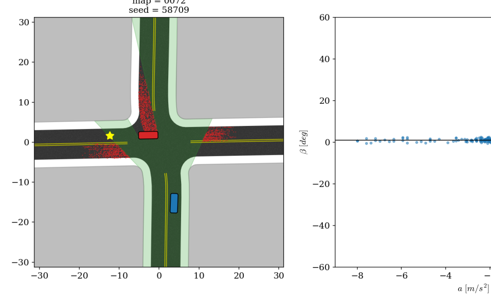
Figure 1: The ego vehicle (blue box) intends to perform an unprotected left turn to the goal (yellow star) at an intersection. The green shaded region is the observable polygon and arises due to the 1) limited sensor range and 2) occlusions from another vehicle (red box) and buildings (gray regions.) The proposed algorithm quantifies and identifies the location of risk posed by other vehicles (red particles). Our approach identifies and focuses its attention on risk-inducing regions in the near future (e.g. 1.5 seconds) to ensure that it does not waste computational resources predicting everything in the occluded region. Both axes are in meters.

In contrast, human drivers can usually handle scenarios like the one in Figure 1 even with relatively limited sensing capabilities, such as a narrow field-of-view. We argue that this is because human drivers sense the world in a more efficient way: using semantic and prior information to focus sensing resources on portions of the scene that are most pertinent. For instance, when driving normally, drivers focus mostly on the current and future location of the ego vehicle. We only glimpse to check the rear view mirror when driving forward, but never focus our attention on it for an extended period of time. This is due to the fact that we have 1) a semantic understanding of the environment (e.g. road layout, speed limit, etc) and 2) prior knowledge such as the ability to estimate the reachability of not only for the ego vehicle but also other agents. As a result, we know to focus our limited sensing resources on only the regions where the ego vehicle can reach, and properly assess the risk to take an action.

This paper proposes an algorithm that leverages this intuition from human driving for probabilistic risk assessment and planning by utilizing not only forward but also backward reachability. Since collisions can only happen within the FRS (FRS) of a vehicle, it is unnecessary to predict everything in the occluded region. Instead, staring from a location in the FRS of the ego vehicle, one can backward propagate the motion of other vehicles and eventually get all possible initial conditions of risky agents. These initial conditions quantifies and spatially identifies risk-inducing regions and agents, as shown in Figure 1. With this information, we show how this quantified risk can be used for motion planning for safe navigation in urban environments.

This paper is organized as follows. Section II reviews related work in reachability-based planning and risk assessment under occlusion. Section III shows our problem formulation and proposed risk assessment and motion planning algorithm based on forward and backward reachability. Section IV describes two baselines and our evaluation metrics. Section V describes the quantitative evaluation of the proposed algorithm and illustrates that the proposed method is a significant improvement over existing methods. Section VI concludes and discusses future directions of this work.

II Related Work

Risk assessment is the process of predicting and quantifying the risk of taking a certain action. The proposed method belongs to the category of methods that quantify the risk of having a collision with another agent in the scene as defined in the well-organized survey by [4].

Reachability-based motion planning is widely used for autonomous driving [5, 6, 7, 8, 9, 10, 11]. [5] assume cooperative agents and proposed an algorithm to negotiate conflicting motions. They try to solve a winner determination problem, which is NP-hard, by restricting the set of combinations to a tree structure. This makes the original problem computationally tractable. [6] over-approximate the FRS of incoming traffic, including those who are occluded, by only considering the leading edge of the observable polygon and make sure that the ego vehicle does not collide with the FRS. [7] use forward reachability to predict future both the FRS of the ego vehicle and the ones of other traffic participants. It performs collision checking of the FRS and is evaluated on both urban intersection and highway scenarios. [8] use both forward and backward reachability, just like the proposed method, to formulate a discrete decision making problem for autonomous driving. [9] propose RTD (RTD) algorithm for real-time trajectory planning in a static scene by showing how to utilize a FRS computed offline during safe online motion planning. [10] later extended the idea [9] to scenes with dynamics agents.

Our approach differs in the following ways. First of all, we formulate the problem probabilistically, whereas the approaches developed by [6, 8, 7, 9, 10] do not. The proposed algorithm captures the distribution of risk in both the action space and Cartesian space thus can be more flexible and gives one to potentially adjust the balance between aggressiveness and effectiveness. Secondly, the work by [8] is intended to be used as a high-level planner for switching between behaviors and thus relies on a low-level planner to generate throttle and steering commands. By contrast, our approach is more like a controller and plans low-level commands directly. Finally, methods by [8, 5, 9, 10] do not consider occlusions or other sensory limitations, whereas our approach is designed to operate even under occlusions.

The algorithm proposed in this paper builds upon our previous work [12], which is also a risk assessment and motion planning algorithm. One weakness of our prior work is its poor scalability with respect to the size of the environment. The computational cost is proportional to the area of the occluded regions within the size of the map. The cost of the new approach proposed in this paper does not scale with the area of occluded regions and has a lower collision rate. Also, our previous approach does not identify where to focus the sensory resource.

The main contributions of this paper are as follows:

• We propose a probabilistic risk assessment method which identifies the location of the risk-inducing agents and regions.

• The proposed method utilizes both forward and backward reachability for efficient risk assessment.

• We show how the quantified risk can be used for motion planning for navigating safely in urban environments.

• We evaluate our method on $73$ real-world intersections and show quantitative improvement in terms of reduced collision rate when compared to the state of the art.

III Method

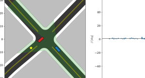
(a)

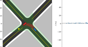
(b)

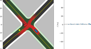
(c)

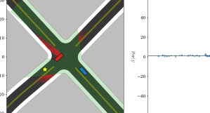
(d)

Figure 2: Step-by-step illustration of different stages of the proposed algorithm. (a) An intersection with occlusion and with one other agent (red box) in the scene. The observable polygon is indicated by the green shaded region, and the goal location is indicated by the yellow star. (b) State 1: calculating FRS_e. The dots are projections of the particles $\left\{x_{e}\left(T^{[i]}\right)\right\}_{i=1}^{N}$ in 2D. (c) Stage 2: calculating BRS_o. The dots are projections of the particles $\left\{x_{o}^{[i]}(0)\right\}_{i=1}^{N}$ in 2D. (d) Stage 3: filtering with the observable polygon. The remaining red dots in the figure indicates spatially the source of risk-inducting regions.

We first define both forward and backward reachability in Section III-A. In Section III-B, we show how to use aforementioned reachability for efficient risk assessment. Finally, in Section III-C, we demonstrate using the quantified risk for motion planning.

III-A Bidirectional Reachability

Let $t\in\mathbb{R}$ be time, $\mathcal{X}$ be the state space and $\mathcal{U}$ be the action space. Let $x(t)\in\mathcal{X}$ be the state and $u(t)\in\mathcal{U}$ be the control input of a dynamic system at time $t$. Assume the vehicle’s dynamics are described as an ODE (ODE):

$$\dot{x}(t)=f(t,x(t),u(t)),$$ (1)

where $f$ is a Lipschitz continuous function.

The FRS describes a set of all possible states of a system in the future. Given the dynamics in (1), an initial set $\mathcal{X}_{0}$ and a fixed time horizon $T$, the FRS is defined as

$$\begin{split}\mbox{FRS}(\mathcal{X}_{0},T):=\{&x(T)\in\mathcal{X}~{}|~{}x_{0}=x(0)\in\mathcal{X}_{0},u(t)\in\mathcal{U},\\ &\dot{x}(t)=f(t,x(t),u(t)),\forall t\in[0,T]\}\end{split}$$ (2)

On the other hand, the BRS (BRS) describes all possible initial states that are able to reach a target set. Given the dynamics in (1), a target set $\mathcal{X}_{f}$ and a fixed time horizon $T$, the BRS is defined as

$$\begin{split}\mbox{BRS}(\mathcal{X}_{f},T):=\{&x(0)\in\mathcal{X}~{}|~{}x_{f}=x(T)\in\mathcal{X}_{f},u(t)\in\mathcal{U}\\ &\dot{x}(t)=f(t,x(t),u(t)),\forall t\in[0,T]\}\end{split}$$ (3)

Normally, reachable sets are calculated for each observed agent [9, 10]. These methods usually perform well when only a limited number of agents are presented in a non-occluded scene. Scenes like urban intersections can still be challenging for these method since predicting everything, especially in a occluded environment, can computationally intensive in many cases. Efforts have been made to ease the calculation under occlusion [6, 12], but the complexity still grows along with either the number of occluded regions [6] or the total area of the occluded regions [12]. For this reason, in Section III-B we introduce multiple stages of our algorithm that utilize both forward and backward reachability for efficient risk assessment under occlusion. The complexity of proposed method stays constant no matter how the number or size of the occluded regions grow.

III-B Risk Assessment

For autonomous driving, collisions happen only at the intersections of the FRS of different agents. In other words, if another agent (occluded or not) cannot reach where the ego vehicle can possibly be in the future, $1.5$ seconds for example, it does not induce risk to the ego vehicle. This observation leads to an important insight – it is unnecessary to predict the behavior of everything in a scene. Instead, we can focus resources on identifying only those agents who pose a risk to the ego vehicle.

The proposed algorithm, whose behavior is depicted in Figure 2, is performed iteratively every $T_{r}$ seconds, and has a forecast horizon of $T_{f}$ seconds. It can be broken down into three stages.

III-B1 Stage 1 – FRS of the Ego Vehicle

In the first stage, the FRS of the ego vehicle is calculated. In particular, we borrow the idea of using particles from our previous work [12, 13] to represent the FRS since it makes the FRS probabilistic and the calculation parallelizable.

Without loss of generality, let $t=0$ at the beginning of each iteration. Let the control inputs be parameterized by some parameters $\theta_{e}$ and $\theta_{o}$ such that

$$\begin{split}u_{e}(t)&=u_{e}\left(t;\theta_{e}\right)\in\mathcal{U}~{}~{}~{}\forall t\\ u_{o}(t)&=u_{o}\left(t;\theta_{o}\right)\in\mathcal{U}~{}~{}~{}\forall t,\end{split}$$ (4)

where the subscripts $e$ and $o$ indicate quantities tailored to the ego vehicle and other vehicles, respectively. Let the $i-$th particle, $p^{[i]}$, be defined as

$$p^{[i]}:=\left\{x_{e}^{[i]}(0),\theta_{e}^{[i]}(t),\theta_{o}^{[i]}(t),T^{[i]}\right\}~{}~{}~{}\forall i=1,\ldots,N,$$ (5)

where the superscript $[i]$ indicates $i-$th sample of a variable, $x_{e}(0)$ is ego vehicle’s initial state, $T$ is a fixed time horizon. and $N$ is the total number of particles.

In each iteration, we first sample $N$ particles from the following distributions:

$$\begin{split}x_{e}(0)&\sim U\left(\mathcal{X}_{e,0}\right)\\ \theta_{e}&\sim P\left(\theta_{e}^{+}~{}|~{}\theta_{e}^{-}\right)\\ \theta_{o}&\sim P\left(\theta_{o}^{+}~{}|~{}\theta_{o}^{-}\right)\\ T&\sim U\left([0,T_{f}]\right),\end{split}$$ (6)

where $\mathcal{X}_{e,0}$ is the initial set of the ego vehicle, $[\cdot,\cdot]$ is a closed interval, $U(\cdot)$ is an uniform distribution over a set, and $P(\cdot^{+}~{}|~{}\cdot^{-})$ is the transition probability of a quantity between subsequent iterations. The transition probabilities enforces smoothness in the action space $\mathcal{U}$ which reduces jittery motion. Since the smoothness is enforced on the distribution level but not directly on the optimal value, actions such as emergency breaking are still allowed. More details about determining the optimal control input from the distribution are described in Section III-C.

Now the probabilistic FRS of the ego vehicle can be re-written as

$$\begin{split}\mbox{FRS}_{e}:=\Big{\{}&x_{e}\left(T^{[i]}\right)\in\mathcal{X}~{}|~{}x_{e}(0)=x_{e,0}^{[i]}\in\mathcal{X}_{e,0}\\ &\dot{x}_{e}(t)=f_{e}\left(t,x_{e}(t),u_{e}^{[i]}(t)\right)\\ &u_{e}^{[i]}(t)\in\mathcal{U},\forall t\in\left[0,T^{[i]}\right]\Big{\}}_{i=1}^{N}\end{split}$$ (7)

The set FRS_e can be easily calculated by solving $N$ IVP in parallel with a regular ODE solver. Note that FRS_e contains $N$ hypotheses of the future states of the ego vehicle, as shown in Figure 2b.

III-B2 Stage 2 – BRS of Other Agents

In the second stage of the proposed algorithm, we calculate the BRS of other agents in a similar fashion by setting the target set $\mathcal{X}_{f}$ to FRS_e such that

$$\begin{split}\mbox{BRS}_{o}:=\Big{\{}&x_{o}(0)\in\mathcal{X}~{}|~{}x_{e}\left(T^{[i]}\right)\in\mbox{FRS}_{e}\\ &\mathcal{P}_{o}\left(x_{o}\left(T^{[i]}\right)\right)=\mathcal{P}_{e}\left(x_{e}\left(T^{[i]}\right)\right)\\ &\dot{x}_{o}(t)=f_{o}\left(t,x_{o}(t),u_{o}^{[i]}(t)\right)\\ &u_{o}^{[i]}(t)\in\mathcal{U},\forall t\in\left[0,T^{[i]}\right]\Big{\}}_{i=1}^{N},\end{split}$$ (8)

where $\mathcal{P}_{o}:\mathcal{X}_{o}\rightarrow\mathbb{R}^{2}$ and $\mathcal{P}_{e}:\mathcal{X}_{e}\rightarrow\mathbb{R}^{2}$ are invertible functions projecting the state spaces into Cartesian space. We use projections since collisions occur when a subset of the states (e.g. positions) overlap. In this case, collision happens at one point in the Cartesian space, while other states such as heading and velocity do not necessary have to be the same and should be assigned separately.

Unlike the FRS_e, the BRS_o set cannot be calculated directly with an ODE solver. Instead, we need to first reformulate the final value problem into an equivalent IVP. For Lipschitz continuous dynamic systems such as CTRV (CTRV) model, CTRA (CTRA) model, and the bicycle model, the initial value $x_{o}(0)$ corresponding to particle $i$ can be obtained by solving the following IVP:

$$\begin{split}\dot{z}(t)&=-f_{o}\left(t,z(t),u_{o}^{[i]}(t)\right)\\ z(0)&=x_{e}\left(T^{[i]}\right)\end{split}$$ (9)

The set BRS_o can now be obtained by solving (9) in parallel with a regular ODE solver, and the solution $z\left(t\right)$ is $x_{o}(t)$ in (8), but reversed in time.

BRS_o represents a collection of risky initial conditions of other agents. Each particle corresponds to a possible collision between the ego vehicle and another agent by design, since the target set of BRS_o is chosen to be FRS_e. By doing so, this approach can handle occlusion in an efficient way. We no longer need to predict all possible agents in the scene. Instead, the set BRS_o originates only from $\mathcal{X}_{e,0}$ and tells us directly where the potentially dangerous agents are, no matter whether they are occluded or not. This step is depicted in Figure 2c.

III-B3 Stage 3 – Consistency with the Observation

BRS_o alone does not quantify the risk associated with a particle. We need to incorporate sensory systems, such cameras, radars and LIDAR, to identify risky control inputs. A combination of the aforementioned sensors generates a free space around the ego vehicle know as the observable polygon, $\mathcal{X}_{s}$, as shown in Figure 2d.

If the entire trajectory of $i-$th particle, $x_{o}^{[i]}(t)$, ends in $\mathcal{X}_{s}$, it is considered to be collision-free; otherwise, it is potentially risky. Quantitatively speaking, a weight $w_{s}^{[i]}$ is assigned to each particle $i$ based on its entire trajectory.

$$w_{s}^{[i]}=\frac{1}{T^{[i]}}\int_{0}^{T^{[i]}}\mathds{1}\left(x_{o}^{[i]}(t)\in\mathcal{X}_{s}\right)dt$$ (10)

where $\mathds{1}(\cdot)$ is an indicator function. As a results, the weight $w_{s}^{[i]}$ renders the likelihood of the corresponding action $u_{e}^{[i]}(t)$ being collision-free or not.

III-C Motion Planning

Based on the weight $w_{s}$ from Section III-B it is possible to generate a set of safe actions by resampling. Resampling the particles with $w_{s}$ defined in (10) filters out actions with potential collision. However, it is insufficient to use just $w_{s}$ during resampling. For example, in many cases the safest action may be stopping completely before reaching the goal or getting up to the target speed. The ego vehicle can freeze and never reaches the goal. Hence we need another factor to promote forward motion of the ego vehicle.

Let $u_{d}$ be the desired control input when no risk is presented in the scene. The desired control input can be from a predefined behavior, such as slowing down gently when approaching an intersection, or maintaining the target speed, etc. Assume that $u_{d}$ is given, we assign another weight $w_{d}$ to each particle.

$$w_{d}^{[i]}:=\exp\left(-\frac{\delta_{u}^{[i]2}}{2\sigma_{u}^{2}}\right)$$ (11)

where

$$\delta_{u}^{[i]2}:=\frac{1}{T^{[i]}}\int_{0}^{T^{[i]}}\left(u_{d}(t)-u_{e}^{[i]}(t)\right)^{\top}\left(u_{d}(t)-u_{e}^{[i]}(t)\right)dt$$

and $\sigma_{u}$ is a hyperparameter for scaling. The weight $w_{d}$ promotes those control inputs which are closer to the desired one, and thus is able to drive the ego vehicle forward.

A naive way to utilize both $w_{s}$ for safety and $w_{d}$ for driving is to interpret them as likelihoods and take their product as the final weight, and resample the particles. However, safe actions might be suppressed when they are no where near the desired action. So taking the direct product may end up with an action that is still too risky.

Instead, we calculate the final weight $w^{[i]}$ in the following way:

$$w^{[i]}=w_{s}^{[i]}\cdot\left(\varepsilon\cdot w_{d}^{[i]}+(1-\varepsilon)\cdot\left(1-\min_{j}w_{s}^{[j]}\right)\right),$$ (12)

where $\varepsilon$ is a small number. We set it to $10^{-4}$ in this paper.

To understand (12) intuitively, let us first consider an extreme case. Assume $w_{s}^{[i]}=1~{}\forall i$, indicating that all the trajectories $x_{o}^{[i]}(t)$ are in the observable polygon $\mathcal{X}_{s}$ ans thus being collision-free. The weight $w^{[i]}$ becomes proportional to $w_{d}^{[i]}$, so the actions closer to the desired action $u_{d}(t)$ will have higher final weights. In this case, resampling with $w^{[i]}$ makes the ego vehicle move according to the desired action.

On the other hand, if any of the trajectories shows slight risk (e.g. $1-\min_{j}w_{s}^{[j]}>10\varepsilon$), the final weight $w^{[i]}$ will be approximately proportional to $w_{s}^{[i]}$. As a result, safer actions get promoted and the value $w_{d}^{[i]}$ has negligible effect in this case. In short, using (12) with a reasonably small $\varepsilon$ forces the ego vehicle to prioritize safety and to move forward only when it is risk-free. Resampling with the weight from (12) gives us a distribution represented by a set of ”good” particles. The final step is to select an optimal control input from this distribution for the ego vehicle to execute.

In general, the distribution can be multi-modal, meaning that there may be multiple control inputs that are equally good. For instance, if there are two vehicles approaching an intersection at the same time, two possibly equally good actions for one of the vehicles can be either 1) being aggressive – accelerating and pass first or 2) being conservative – waiting until the other one passes. For this reason, we make use of a well-developed clustering algorithm from the machine learning and computer vision community – DBSCAN (DBSCAN) [14] – to identify multi-modal distributions and select the optimal action.

DBSCAN clusters particles in the action space based on the local density without specifying the number of clusters a priori. It identifies the number of cluster automatically, and the centroids of clusters are candidates for the optimal control input. We choose to prioritize safety and make the ego vehicle to be more conservative in this paper. So if there are multiple clusters, we pick the one with the most deceleration. The optimal control input is then executed until the next iteration.

IV Evaluation

This section introduces the baselines for the proposed algorithm to be compared against. We also define the metrics for evaluation.

IV-A Model

Section III-B only gives a general description of the pipeline for clarity, but to test and implement the proposed algorithm, we need to pick appropriate models for both the ego vehicle and other vehicles. Due to its simplicity and tractable dimension, we choose to use the train-like model, meaning that all the agents travels in their own curvilinear coordinates. A concrete example of the model is to have a vehicle traveling on a lane without lane changing. Although we assume no lane changing in this work, it is possible to relax this constraint by using physics-based model like the bicycle model or other behaviour-based models.

By working in curvilinear coordinates, the location of the ego vehicle can be parameterized by only two numbers: longitudinal position $s_{e}$ along the center line and the lateral offset $b_{e}$ with respect to the center line. In addition, the heading is completely determined by $s_{e}$ thus is not necessary to be included as a state. The dynamics of the ego vehicle can be written as

$$\begin{split}\dot{x}_{e}(t)&=\begin{bmatrix}0&1\\ 0&0\end{bmatrix}x_{e}(t)+\begin{bmatrix}0\\ 1\end{bmatrix}u_{e}(t)\\ x_{e}(t)&:=\begin{bmatrix}s_{e}(t)&\dot{s}_{e}(t)\end{bmatrix}^{\top}\\ u_{e}(t)&:=a_{e}~{}~{}~{}\forall t\geq 0,\end{split}$$ (13)

where $a_{e}$ is a constant acceleration along the center line. The dynamics of other vehicles is written in a similar way, but assumed to have a constant speed $v_{o}$ such that

$$\begin{split}\dot{x}_{o}(t)&=u_{o}(t)\\ x_{o}(t)&:=s_{o}(t)\\ u_{o}(t)&:=v_{o}~{}~{}~{}\forall t\geq 0\end{split}$$ (14)

If there are multiple valid lanes for non-ego vehicles, each lane should have its own dynamics.

Here we want to emphasize that more sophisticate models can be substituted in directly, but at the cost of higher computational complexity. We choose constant speed/acceleration models because their simplicity and reasonable performance in similar scenarios, as illustrated in our previous work [12]. Moreover, since we work in curvilinear coordinates, both models, (13) and (14), can be approximated by CTRV and CTRA models, respectively, when the replanning time $T_{r}$ is small. Both CTRV and CTRA are shown to have comparable performance in prediction in urban environments [15].

The desired action $u_{d}(t)$ is designed to have a constant deceleration when approaching the stopline, and to switch to a saturating proportional controller to track a target speed.

IV-B Baseline 1

The first baseline is an occlusion-aware algorithm by [6]. We recreate and simulate two of the scenarios demonstrated in their paper. The map is a four-way unsignalized intersection partially occluded by a non-transparent static object.

The first scenario consists of no other agent, and the second one has one other agent coming from the left hand side of the ego vehicle. In both scenarios, the goal is to navigate safely through the intersection and to reach a target speed of $9~{}m/s$. The geometries of the map are measured using AutoCAD, and the velocity of the other agent is estimated afterwards.

IV-C Baseline 2

The second baseline is another occlusion-aware method from our previous work [12]. We simulate the same set of $1000$ random scenarios with up to five other agents for each scene on both the proposed method and the second baseline. Each scene is an four-way unsignalized intersection and the geometries are extracted from OSM (OSM). There are $73$ real-world intersections in total. In addition, there is also a synthetic layout where the roads are straight and perpendicular to each other.

These maps have significantly more severe occlusion comparing to those in the first baseline [6]. Buildings are added to the map with a two-meter buffer around the driving surface, as shown in Figure 1 and 2. Speed of a non-ego agent is randomly set to a constant between $4$ to $12~{}m/s$. For simplicity, we assume no collision between non-ego agents and they do not interact with other agents.

(a)

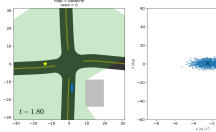
(b)

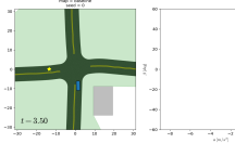
(c)

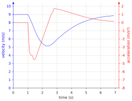
(d) Baseline 1 [6]

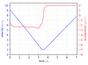
(e) Proposed

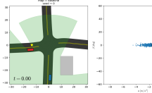
(f)

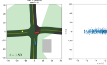
(g)

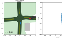
(h)

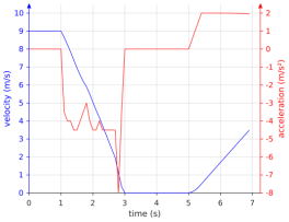
(i) Baseline 1 [6]

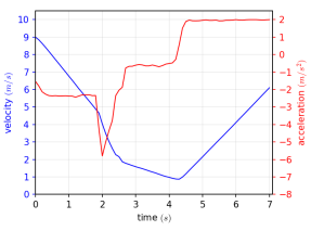
(j) Proposed

Figure 3: Two scenarios in the first baseline [6]. The first scenario (top row) is in a map with one static obstacle (gray) and no incoming traffic, and the second scenario (bottom row) is in the same map with one other vehicle (red) coming from the left. The first three columns (a-c, f-h) show key frames of the proposed method, and the other two columns (d,e,i,j) show the speed and acceleration profiles. In the first scenario, the baseline abruptly breaks at $t=1.0s$ whereas the proposed method maintains a near constant deceleration, as shown in (d) and (e). In the second scenario, the baseline breaks at both $t=1.0s$ and $t=2.8s$, whereas the proposed method only breaks once at $t=1.9s$, as shown in (i) and (j). In addition our method does not stop completely in the second scenario. Instead, it creeps forward between $t=2.7s$ and $t=4.3s$ to gather more information. This behavior results in a higher final speed and thus makes the ego vehicle faster to reach the goal. The fourth column is adopted directly from Figure 4 in [6].

IV-D Metrics

For the first baseline, we investigate the speed and acceleration profiles for both ride comfort and efficiency. Ride comfort is evaluated by the number of abrupt breaking and the maximum deceleration, whereas efficiency is indicated by the terminal speed of the ego vehicle.

Collision rate is evaluated for the second baseline on one synthetic and all the $73$ real-world intersections. This results in $74000$ simulations in total for each method.

V Results

V-A Baseline 1

Figure 3 shows the behaviors under two scenarios recreated from the first baseline [12]. Both the first baseline and the proposed method enable the ego vehicle to reach to the goal without collision in either scenario. The ego vehicle slows down when approaching the intersection, no matter if there is any incoming traffic.

However, they have three key differences. To begin with, in the first scenario the baseline [6] has a sudden break at $t=1.0s$, while the proposed method stays roughly at a constant deceleration. In addition, the maximum breaking (i.e. deceleration) in the second scenario is $27.5\%$ lower in the proposed method. The reduced breaking and jerk indicate higher ride comfort. Finally, in the second scenario the ego vehicle creeps forward between $t=2.7s$ and $t=4.3s$ in order to get a clearer view, as shown in Figure 3h and 3j. Once it gets enough information and thinks it is risk-free, it then proceeds. This behavior leads to a higher efficiency, meaning that it obtains a $57.9\%$ higher speed at the end of the simulation all without sacrificing safety.

V-B Baseline 2

	median collision rate	# of zero-collision intersections
Baseline 2 [12]	$1.70\%$	$0$ out of $74$
Proposed	$0.20\%$	$10$ out of $74$

TABLE I: Simulation results at $74$ intersections.

Among the $74$ intersections, the proposed method obtains a median collision rate of $0.20\%$, which is a significant reduction compared to the $1.70\%$ of the second baseline [12], as shown in Table I. Moreover, the proposed method achieves zero collision at not only the synthetic layout, but also $9$ real-world layouts. In contrast, the baseline [12] has a minimum collision rate of $0.70\%$ at one of the $74$ intersections.

VI Conclusions and Future Work

We propose a probabilistic risk assessment method for motion planning under occlusion in urban intersections. The proposed algorithm is able to quantify the distribution of risk in the action space, and can be used to generate low-level control inputs for an autonomous vehicle to navigate safely. It also identifies spatially where the risk-inducing regions are via both forward and backward reachability. The proposed method is compared quantitatively to previous work and shows significant improvement in terms of both efficiency and safety.

Future work include using the proposed method to redirect and focus sensory resources to further reduce impact on limited sensing, formulating and solving the problem analytically without sampling to obtain safety guarantees, and deploying it to hardware platforms for testing in the real-world.

References

- [1] S. Kato et al. “An Open Approach to Autonomous Vehicles” In IEEE Micro 35.6, 2015, pp. 60–68 DOI: 10.1109/MM.2015.133
- [2] M. Lee, K. Jo and M. Sunwoo “Collision risk assessment for possible collision vehicle in occluded area based on precise map” In IEEE 20th International Conference on Intelligent Transportation Systems (ITSC), 2017, pp. 1–6 DOI: 10.1109/ITSC.2017.8317666
- [3] S. Ammoun and F. Nashashibi “Real time trajectory prediction for collision risk estimation between vehicles” In 2009 IEEE 5th International Conference on Intelligent Computer Communication and Processing, 2009, pp. 417–422 DOI: 10.1109/ICCP.2009.5284727
- [4] Stéphanie Lefèvre, Dizan Vasquez and Christian Laugier “A survey on motion prediction and risk assessment for intelligent vehicles” In ROBOMECH Journal 1.1, 2014, pp. 1 DOI: 10.1186/s40648-014-0001-z
- [5] S. Manzinger and M. Althoff “Tactical Decision Making for Cooperative Vehicles Using Reachable Sets” In 2018 21st International Conference on Intelligent Transportation Systems (ITSC), 2018, pp. 444–451 DOI: 10.1109/ITSC.2018.8569560
- [6] P. F. Orzechowski, A. Meyer and M. Lauer “Tackling Occlusions Limited Sensor Range with Set-based Safety Verification” In 2018 21st International Conference on Intelligent Transportation Systems (ITSC), 2018, pp. 1729–1736 DOI: 10.1109/ITSC.2018.8569332
- [7] M. Koschi and M. Althoff “SPOT: A tool for set-based prediction of traffic participants” In 2017 IEEE Intelligent Vehicles Symposium (IV), 2017, pp. 1686–1693 DOI: 10.1109/IVS.2017.7995951
- [8] H. Ahn, K. Berntorp and S. Di Cairano “Reachability-based Decision Making for City Driving” In 2018 Annual American Control Conference (ACC), 2018, pp. 3203–3208 DOI: 10.23919/ACC.2018.8431819
- [9] S. Vaskov et al. “Guaranteed Safe Reachability-based Trajectory Design for a High-Fidelity Model of an Autonomous Passenger Vehicle” In 2019 American Control Conference (ACC), 2019, pp. 705–710
- [10] Sean Vaskov et al. “Towards Provably Not-at-Fault Control of Autonomous Robots in Arbitrary Dynamic Environments” In CoRR abs/1902.02851, 2019 arXiv: http://arxiv.org/abs/1902.02851
- [11] Andrea Bajcsy et al. “An Efficient Reachability-Based Framework for Provably Safe Autonomous Navigation in Unknown Environments” In arXiv preprint arXiv:1905.00532, 2019
- [12] M. Yu, R. Vasudevan and M. Johnson-Roberson “Occlusion-Aware Risk Assessment for Autonomous Driving in Urban Environments” In IEEE Robotics and Automation Letters 4.2, 2019, pp. 2235–2241 DOI: 10.1109/LRA.2019.2900453
- [13] Henry O Jacobs, Owen K Hughes, Matthew Johnson-Roberson and Ram Vasudevan “Real-time certified probabilistic pedestrian forecasting” In IEEE Robotics and Automation Letters 2.4 IEEE, 2017, pp. 2064–2071
- [14] Martin Ester, Hans-Peter Kriegel, Jörg Sander and Xiaowei Xu “A density-based algorithm for discovering clusters in large spatial databases with noise” AAAI Press, 1996, pp. 226–231
- [15] R. Schubert, E. Richter and G. Wanielik “Comparison and evaluation of advanced motion models for vehicle tracking” In 2008 11th International Conference on Information Fusion, 2008, pp. 1–6