Validating the methodology for constraining the linear growth rate from clustering anisotropies

Abstract

Redshift-space clustering distortions provide one of the most powerful probes to test the gravity theory on the largest cosmological scales. We perform a systematic validation study of the state-of-the-art statistical methods currently used to constrain the linear growth rate from redshift-space distortions in the galaxy two-point correlation function. The numerical pipelines are tested on mock halo catalogues extracted from large N-body simulations of the standard cosmological framework. We consider both the monopole and quadrupole multipole moments of the redshift-space two-point correlation function, as well as the radial and transverse clustering wedges, in the comoving scale range $10<r[$$h^{-1}\,\mbox{Mpc}$$]<55$. Moreover, we investigate the impact of redshift measurement errors on the growth rate and linear bias measurements due to the assumptions in the redshift-space distortion model. Considering both the dispersion model and two widely-used models based on perturbation theory, we find that the linear growth rate is underestimated by about $5-10\%$ at $z<1$, while limiting the analysis at larger scales, $r>30$ $h^{-1}\,\mbox{Mpc}$, the discrepancy is reduced below $5\%$. At higher redshifts, we find instead an overall good agreement between measurements and model predictions. Though this accuracy is good enough for clustering analyses in current redshift surveys, the models have to be further improved not to introduce significant systematics in RSD constraints from next generation galaxy surveys. The effect of redshift errors is degenerate with the one of small-scale random motions, and can be marginalised over in the statistical analysis, not introducing any statistically significant bias in the linear growth constraints, especially at $z\geq 1$.

1 Introduction

Over the past decades, we witnessed progressive improvements in the field of observational cosmology, for what concerns both data acquisition and modelling. Exploiting various independent cosmological probes, the so-called standard $\Lambda$-cold dark matter ($\mathrm{\Lambda CDM}$) model has been constrained with high levels of accuracy and precision. Several projects have been carried on to explore the properties of cosmic tracers at different scales, with the primary goal of understanding the formation and evolution of the Universe. The main properties of the large-scale structure of the Universe have been constrained both at very high redshifts, exploiting the Cosmic Microwave Background (CMB) power spectrum (Bennett et al., 2013; Planck Collaboration et al., 2018), and in the local Universe thanks to increasingly large surveys of galaxies and galaxy clusters (e.g. Parkinson et al., 2012; Campbell et al., 2014; Guzzo et al., 2014; Alam et al., 2017; Pacaud et al., 2018).

The unprecedented amount and quality of the data expected from the upcoming projects will allow us to test fundamental physics, shedding light on questions that have remained unanswered for years. In particular, in the era of huge galaxy survey projects, such as the Dark Energy Survey (DES) (DES Collaboration et al., 2017), the extended Roentgen Survey with an Imaging Telescope Array (eROSITA) satellite mission (Merloni et al., 2012), the NASA Wide Field Infrared Space Telescope (WFIRST) mission (Spergel et al., 2013), the ESA Euclid mission (Laureijs et al., 2011; Amendola et al., 2018), the Large Synoptic Survey Telescope (LSST) (Ivezic et al., 2008), and the Square Kilometre Array (SKA) (Maartens et al., 2015; Santos et al., 2015), we will have the opportunity to clarify some of the main issues in the current understanding of the Universe, such as the physical nature of dark matter (DM) and dark energy (DE), and to test the gravity theory on the largest scales accessible (for a recent review see e.g. Silk, 2017). In fact, about $95\%$ of the content of the Universe still remains with an unsatisfactory physical explanation. This represents the main motivation for the forthcoming generation of galaxy surveys, whose main goal is to achieve a better understanding of the nature of DM and DE components. Increasingly large and accurate maps of galaxies and other cosmic tracers will be exploited to probe the expansion history of the Universe and the formation of cosmic structures with unprecedented accuracy, allowing us to robustly discriminate among alternative cosmological frameworks.

In this context, one of the most powerful tools to characterise the spatial distribution of cosmic tracers is provided by the two-point correlation function (2PCF), or analogously the power spectrum, which encodes most of the information available. In particular, the so-called redshift-space distortions (RSD) in the tracer clustering function (Jackson, 1972; Kaiser, 1987; Hamilton, 1998; Scoccimarro, 2004) have been effectively exploited to test the gravity theory on cosmological scales, providing robust constraints on the linear growth rate of cosmic structure, using different techniques in both configuration space (e.g. Guzzo et al., 2000; Reid et al., 2012; Beutler et al., 2012; Samushia et al., 2012; Chuang & Wang, 2013; Chuang et al., 2013; de la Torre et al., 2013; Samushia et al., 2014; Howlett et al., 2015; Okumura et al., 2016; Chuang et al., 2016; Pezzotta et al., 2017; Mohammad et al., 2018) and Fourier space (e.g. Tojeiro et al., 2012; Blake et al., 2012, 2013; Beutler et al., 2014). Linear growth rate constraints have been also obtained from the joint analysis of galaxy clustering and weak gravitational lensing (e.g. de la Torre et al., 2017), from cosmic void profiles (e.g. Hamaus et al., 2016; Achitouv et al., 2017; Hawken et al., 2017), and from other different tracers of the peculiar velocity field (e.g. Percival et al., 2004; Davis et al., 2011; Feix et al., 2015; Huterer et al., 2017; Adams & Blake, 2017). Moreover, it has been shown that RSD provide a powerful probe to constrain the mass of relic cosmological neutrinos (Marulli et al., 2011; Upadhye, 2019) and the main parameters of interacting DE models (Marulli et al., 2012a; Costa et al., 2017), as well as help in breaking the degeneracy between modified gravity and massive neutrino cosmologies (Moresco & Marulli, 2017; Wright et al., 2019; García-Farieta et al., 2019).

In this paper, we present a systematic validation analysis of the main statistical techniques currently used to constrain the linear growth rate from redshift-space anisotropies in the 2PCF of cosmic tracers. In Bianchi et al. (2012) and Marulli et al. (2012b); Marulli et al. (2017) we performed a similar investigation, testing RSD likelihood modules on large mock catalogues extracted from N-body simulations of the standard cosmological framework. Here we extend these previous studies in many important aspects. First, instead of modelling the two-dimensional 2PCF, we consider either the monopole and quadrupole multipole moments of the 2PCF, or the clustering wedges, which encode most of the information in the large-scale structure distribution. Moreover, we investigate new RSD models based on perturbation theory, namely the Scoccimarro (2004) and Taruya et al. (2010) models, that we compare to the so-called dispersion model (Davis & Peebles, 1983; Peacock & Dodds, 1996). As in Marulli et al. (2012b), we investigate also the impact of redshift measurement errors, which introduce spurious small-scale clustering anisotropies. We focus on the redshift range $0.5\lesssim z\lesssim 2$, and consider mildly non-linear scales $10<r[$$h^{-1}\,\mbox{Mpc}$$]<55$, where the assumptions in the RSD models considered in this work are expected to be reliable. In addition, we investigate the impact of considering only larger scales, $r>30$ $h^{-1}\,\mbox{Mpc}$, where the models are supposed to be less biased.

The paper is structured as follows. In Section 2 we describe the set of N-body simulations employed in the analysis, and the selected mock DM halo samples. In Section 3, we analyse the clustering of DM haloes in real and redshift space, investigating the impact of redshift measurement errors. The RSD likelihood models and the linear growth rate and bias measurements are presented in Section 4. Finally, in Section 5, we draw our conclusions.

2 N-body simulations and mock halo catalogues

We consider a subset of the DM halo catalogues extracted from the publicly available MDPL2 N-body simulations, which belong to the MultiDark suite (Riebe et al., 2013; Klypin et al., 2016), that is available at the CosmoSim database. These simulations have been widely used in recent years for different cosmological analyses (see e.g. van den Bosch & Jiang, 2016; Rodríguez-Puebla et al., 2016; Klypin et al., 2016; Vega-Ferrero et al., 2017; Zandanel et al., 2018; Topping et al., 2018; Wang et al., 2018; Ntampaka et al., 2019; Granett et al., 2019). The MDPL2 simulations followed the dynamical evolution of $3840^{3}$ DM particles, with mass resolution of $1.51\times 10^{9}h^{-1}\,M_{\odot}$, in a comoving box of $1000$$h^{-1}\,\mbox{Mpc}$  on a side, assuming a $\mathrm{\Lambda CDM}$ framework consistent with Planck constraints (Planck Collaboration et al., 2014, 2016): $\Omega_{m}=0.307$, $\Omega_{\Lambda}=0.693$, $\Omega_{b}=0.048$, $\sigma_{8}=0.823$, $n=0.96$ and $h=0.678$. The DM haloes (Riebe et al., 2013) have been identified with a Friends-of-Friends (FoF) algorithm with a linking length of $0.2$ times the mean interparticle distance (Knebe et al., 2011).

For the clustering analysis presented in this paper we make use of one realisation of the halo samples per each redshift considered, selecting only DM haloes with more than $665$ particles, which corresponds to a minimum mass threshold of $M_{\rm min}=10^{12}h^{-1}\,M_{\odot}$. The samples have been restricted in the mass range $M_{\rm min}<M<M_{\rm max}$, where $M_{\rm max}=2\times 10^{15},1.3\times 10^{15},7.4\times 10^{14},5.4\times 10^{14},4.0\times 10^{14},3.6\times 10^{14},3.1\times 10^{14}h^{-1}\,M_{\odot}$, at $z=0.523,\leavevmode\nobreak\ 0.740,\leavevmode\nobreak\ 1.032,\leavevmode\nobreak\ 1.270,\leavevmode\nobreak\ 1.535,\leavevmode\nobreak\ 1.771,\leavevmode\nobreak\ 2.028$, respectively. These DM haloes are more massive than the ones tipically hosting the faintest galaxies that will be detected in next-generation surveys, like e.g. Euclid and DESI. The non-linear RSD effects are sensitive to the tracer bias, and systematic model uncertainties are expected to be larger for lower bias tracers. Thus, the performances of the considered RSD models on forthcoming clustering measurements might be worse than the ones obtained in this paper. Higher resolution simulations and more realistic mock galaxy catalogues are required to test this hypotesis.

3 Clustering of DM haloes

In this Section, we describe the methodology used to quantify the halo clustering through the 2PCF, which constitutes the main subject of our study. Specifically, we characterise the anisotropic clustering either with the first two non-null multipole moments of the 2PCF, or with the clustering wedges. All numerical computations in the current Section and in the following ones have been performed with the CosmoBolognaLib, a large set of free software libraries (Marulli et al., 2016).

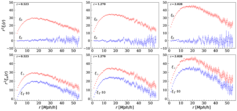
Figure 1: The real-space 2PCF of DM haloes at three different redshifts, as indicated by the labels. Upper panels: the monopole, $\xi_{0}$, and quadrupole, $\xi_{2}$, moments. Bottom panels: the perpendicular, $\xi_{\perp}$, and parallel, $\xi_{\parallel}$, wedges; the latter are shifted by $-10$, for clarity reasons. The error bars are computed with bootstrap sampling.

3.1 The 2PCF

We characterise the spatial distribution of DM haloes in the MDPL2 simulations with the 2PCF in both real space, $\xi(r,\mu)$, and redshift space, $\xi(s,\mu)$. Specifically, we measure the full 2D 2PCF with the conventional Landy & Szalay (1993) estimator:

$$\hat{\xi}(r,\mu)=\frac{DD(r,\mu)-2DR(r,\mu)+RR(r,\mu)}{RR(r,\mu)}\,,$$ (1)

with $\mu$ being the cosine of the angle between the line-of-sight (LOS) and the comoving separation $r$, and $DD(r,\mu),RR(r,\mu)$, and $DR(r,\mu)$ being the normalised number of pairs of DM haloes in data-data, random-random and data-random catalogues, respectively. We measure the 2PCF in the scale range from $1$ to $55$$h^{-1}\,\mbox{Mpc}$, in $80$ linearly spaced bins, with random samples five times larger than the halo ones, to keep the shot noise errors due to the finite number of random objects negligible.

The clustering anisotropies can be effectively quantified by decomposing the full 2D 2PCF either in its multipole moments or in the so-called wedges (Kazin et al., 2012; Sánchez et al., 2013, 2014, 2017). In terms of the first non-vanishing Legendre multipole moments, the 2D 2PCF is written as follows:

$$\xi(s,\mu)=\xi_{0}(s)L_{0}(\mu)+\xi_{2}(s)L_{2}(\mu)+\xi_{4}(s)L_{4}(\mu)\,,$$ (2)

where $L_{l}(\mu)$ are the Legendre polynomials of degree $l$ (i.e. $L_{0}=1$,  $L_{2}=(3\mu^{2}-1)/2$, $L_{4}=(35\mu^{4}-30\mu^{2}+3)/8$), and the coefficient of the expansion corresponds to the $l^{th}$ multipole moment of the 2PCF:

$$\xi_{l}(s)\equiv\frac{2l+1}{2}\int_{-1}^{+1}\,\mbox{d}\mu\,\xi(s,\mu)L_{l}(\mu)\,.$$ (3)

In this work we measure the multipole moments through the direct estimator, performing the pair-counting directly in 1D bins, instead of integrating over 2D bins as in the integrated estimator. This is convenient to avoid uncertainties due to binning effects in the numerical integration, and to optimise computational performances. Since our random pairs do not depend on $\mu$, i.e. $RR(r,\mu)=RR(r)$, the two estimators provide the same results (Kazin et al., 2012; Marulli et al., 2018, e.g.). In real space the full clustering signal is encoded in the monopole moment, $\xi_{0}(r)$. In redshift space the odd multipole moments vanish by symmetry at first order. Here we focus on the first two non-null multipole moments, that is the monopole $\xi_{0}(s)$ and the quadrupole $\xi_{2}(s)$.

An alternative description of the clustering anisotropies is provided by the clustering wedges, introduced by Kazin et al. (2012), that correspond to the angle-averaged of the $\xi(s_{\perp},s_{\parallel})$ over wide bins of $\mu$:

$$\xi_{w}(s)\equiv\frac{1}{\Delta\mu}\int_{\mu_{1}}^{\mu_{2}}\xi(s,\mu)\mathrm{d}\mu\,,$$ (4)

where $\Delta\mu=\mu_{2}-\mu_{1}$ is the wedge width. In this work we consider the two clustering wedges with $\Delta\mu=0.5$, that is the transverse wedge, $\xi_{\perp}(s)\equiv\xi_{1/2}(\mu_{min}=0,s)$, and the radial (or LOS) wedge, $\xi_{\parallel}(s)\equiv\xi_{1/2}(\mu_{min}=0.5,s)$, computed in the ranges $0\leq\mu<0.5$ and $0.5\leq\mu\leq 1$, respectively. The clustering wedges are related to the multipole moments through the following equation:

$$\xi_{w}(r)=\sum_{l}\xi_{l}(s)\bar{L}_{l}\,,$$ (5)

where $\bar{L}_{l}$ is the average value of the Legendre polynomials over the interval $[\mu_{1},\mu_{2}]$. Neglecting contributions from multipoles with $l>2$ and wedge width $\Delta\mu=0.5$, Eq. (5) can be approximated as follows (Kazin et al., 2012):

$$\left(\begin{array}[]{l}{\xi_{\|}}\\ {\xi_{\perp}}\end{array}\right)=\left(\begin{array}[]{cc}{1}&{\frac{3}{8}}\\ {1}&{-\frac{3}{8}}\end{array}\right)\left(\begin{array}[]{c}{\xi_{0}}\\ {\xi_{2}}\end{array}\right)\,.$$ (6)

In real space, the radial and transverse wedges are identical, and equal to the monopole, since there are no distortions in any direction.

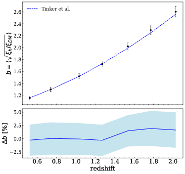
Figure 2: Left panel: the effective halo bias as a function of the comoving scale, at three different redshifts, as indicated by the labels. Dashed lines show the theoretical $\mathrm{\Lambda CDM}$ effective bias predicted by Tinker et al. (2008, 2010), while solid lines show the best-fit bias obtained from the measurements. Right panel: the mean effective halo bias as a function of redshift, computed by averaging in the scale range $10<r[$$h^{-1}\,\mbox{Mpc}$$]<50$. The dashed line shows the Tinker et al. (2008, 2010) prediction. The deviation between measured and theoretical effective bias values is reported in the bottom panel, where the shaded blue area represents the propagated measurement errors.

The errors on the 2PCF measurements are estimated by using the bootstrap resampling method (Efron, 1979). Firstly, the original catalogue is divided into $27$ sub-samples, which are then re-sampled in $100$ different data sets with replacement, then the $\xi(r,\mu)$ is measured in each one of them (Barrow et al., 1984; Ling et al., 1986). The covariance matrix, $C_{k}(s_{i},s_{j})$, is computed as follows:

$$C_{k}\left(s_{i},s_{j}\right)=\frac{1}{N_{R}-1}\sum_{n=1}^{N_{R}}\left[\xi_{k}^{n}\left(s_{i}\right)-\overline{\xi}_{k}\left(s_{i}\right)\right]\left[\xi_{k}^{n}\left(s_{j}\right)-\overline{\xi}_{k}\left(s_{j}\right)\right]\,.$$ (7)

The indices $i$ and $j$ run over the 2PCF bins, while $k$ refers either to the order of the multipole moments considered, in which case $k=l=0,\leavevmode\nobreak\ 2$, or to the clustering wedges, with $k=w=0,\leavevmode\nobreak\ 0.5$. In both cases, $\bar{\xi}_{k}=1/N_{R}\sum_{n=1}^{N_{R}}\xi_{k}^{n}$ is the average multipole (wedge) of the 2PCF, and $N_{R}=100$ is the number of realisations obtained by resampling the catalogues with the bootstrap method. We do not correct the inverse covariance matrix estimator to account for the finite number of realisations (Hartlap et al., 2007). This is not crucial in the context of the present work, which is focused on systematic errors caused by approximations in RSD models.

3.2 Clustering in real space

Figure 1 shows the real-space 2PCF of DM haloes at three different redshifts. The upper panels show the multipole moments, namely monopole, $\xi_{0}(r)$, and quadrupole, $\xi_{2}(r)$. As expected, the real-space monopole moment contains the full clustering signal, while the real-space quadrupole moment is consistent with zero, at $1\sigma$, at all scales. The lower panels show the perpendicular, $\xi_{\perp}(r)$, and parallel, $\xi_{\parallel}(r)$, clustering wedges. The latter are shifted by $-10$ for visualisation purposes. As mentioned before and as confirmed by our results, the two wedges are statistically equal in real space, for isotropy, and equal to the monopole moment. In all cases, the error bars are computed with the bootstrap method.

The amplitude of the real-space clustering signal allows us to characterise the effective halo bias, $b_{\rm eff}$, which relates the halo clustering to the underlying mass distribution. Specifically, $b_{\rm eff}$ can be estimated as follows:

$$\left\langle b_{\rm eff}(z)\right\rangle=\left\langle\sqrt{\frac{\xi_{\rm halo}}{\xi_{\rm DM}}}\leavevmode\nobreak\ \right\rangle\,,$$ (8)

where $\xi_{\rm halo}$ is the measured 2PCF of the MDPL2 DM haloes, while the DM 2PCF, $\xi_{\rm DM}$, is computed by Fourier transforming the non-linear matter power spectrum obtained with CAMB (Lewis et al., 2000), which includes HALOFIT (Smith et al., 2003; Takahashi et al., 2012). The bias is averaged in the scale range $10<r[$$h^{-1}\,\mbox{Mpc}$$]<55$.

The left panel of Fig. 2 shows the measured DM halo bias as a function of scale, with error bars propagated from the 2PCF. The dashed blue lines correspond to the theoretical prediction computed by averaging the linear bias, $b(M,z)$, of the selected set of DM haloes as follows:

$$b_{\rm eff}(z)=\frac{\int_{M_{\rm min}}^{M_{\rm max}}n(M,z)b(M,z)dM}{\int_{M_{\rm min}}^{M_{\rm max}}n(M,z)dM},$$ (9)

where the mass limits $[M_{\rm min}$, $M_{\rm max}]$ have been defined in Section 2, while the mass function, $n(M,z)$, and the linear bias, $b(M,z)$, are estimated using the Tinker et al. (2008) model and the Tinker et al. (2010) model, respectively. The solid black lines show the best-fit bias obtained from the measurements.

A scale-dependent behaviour of the bias can be appreciated at scales smaller than $10$$h^{-1}\,\mbox{Mpc}$, with deviations of about $4$% with respect to the theoretical linear predictions. We note that at these small scales the assumed DM power spectrum model might not be accurate enough, considering the measurement clustering uncertainties of this analysis. Thus the observed scale dependence of the bias might be partially caused by model systematics. However, this does not affect our results, as we do not consider these scales in our analysis. The right panel of Fig. 2 shows the redshift evolution of the mean effective bias, compared to the theoretical $\mathrm{\Lambda CDM}$ predictions by Tinker et al. (2008, 2010). The error bars are computed by propagating the 2PCF errors estimated with bootstrap resampling. Measurements appear in excellent agreement with theoretical expectations.

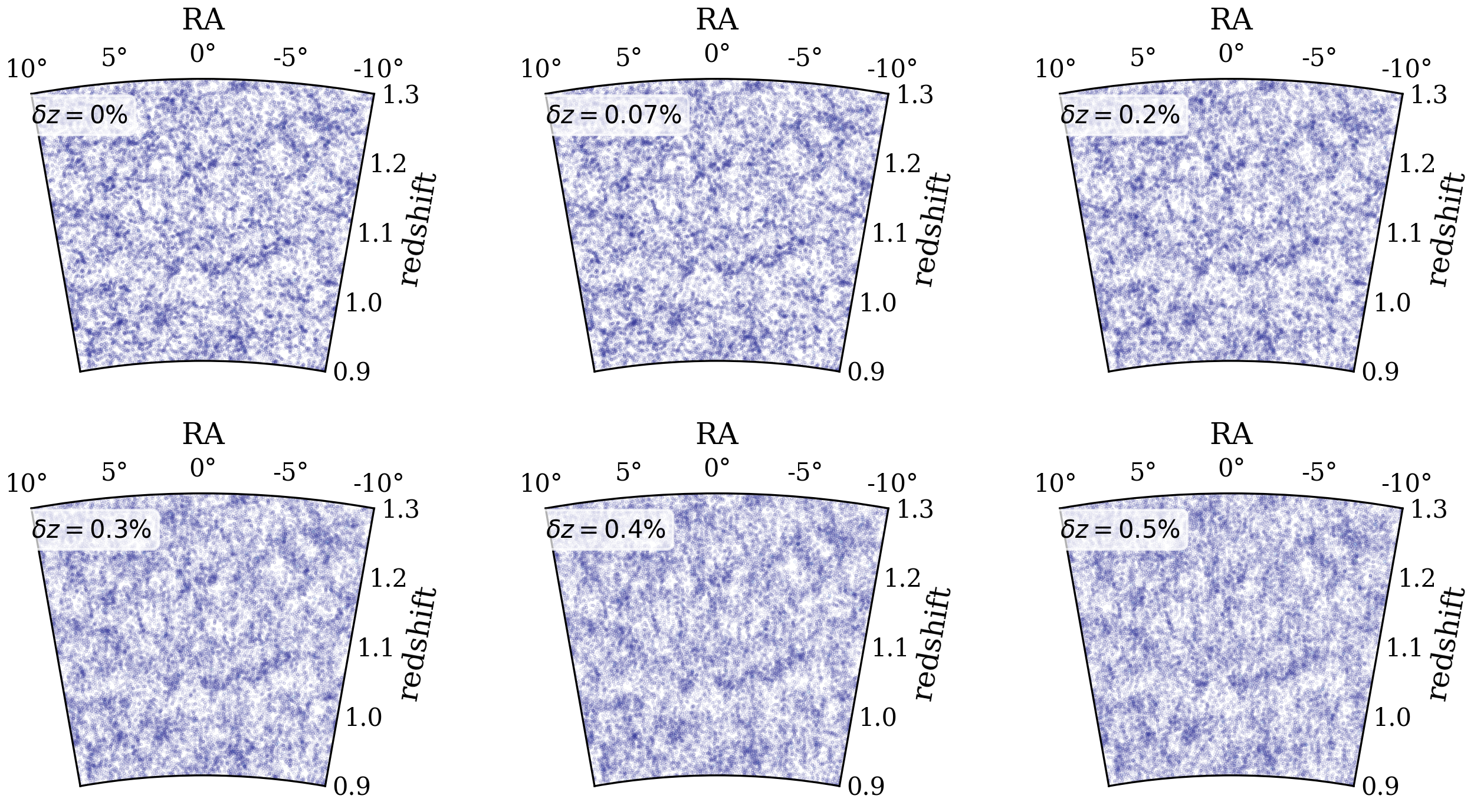
Figure 3: Spatial distribution of DM haloes in the mock sample corresponding to the N-body snapshot at $z=1.032$, including redshift measurement errors, as indicated by the labels. Only haloes in a $2$ degree declination slice are plotted, for clarity.

3.3 Clustering in redshift space and dynamic distortions

When comoving distances are estimated from observed redshifts, $z_{\rm obs}$, without correcting for the LOS peculiar velocity contribution, the resulting clustering pattern appears distorted. These clustering anisotropies are known as dynamic distortions, or RSD. Specifically, $z_{\rm obs}$ can be approximated as a combination of three terms (e.g. Marulli et al., 2012b): i) the cosmological redshift, $z_{c}$, due to the Hubble flow, ii) the change caused by the peculiar velocity along the LOS, and iii) an additional term due to the redshift measurement errors coming from the adopted instrumentation and calibration analysis. Neglecting the latter two terms introduces displacements between the matter distribution in real and redshift space (for a review see Hamilton, 1998; Scoccimarro, 2004).

We construct mock halo catalogues in redshift space following the same procedure adopted by Marulli et al. (2012b); Marulli et al. (2017). First, we introduce a local observer at a random position in the simulation. Then we transform the comoving coordinates of each DM halo into polar coordinates, and estimate the observed redshifts assuming the following relation:

$$z_{\rm obs}=z_{c}+(1+z_{c})\frac{\mathbf{v}\cdot\hat{\mathbf{x}}}{c}\hat{\mathbf{x}}+\frac{\sigma_{v}}{c}\,,$$ (10)

where $\hat{\mathbf{x}}$ is a unit vector along the LOS, and $\sigma_{v}$ corresponds to the amplitude of a Gaussian noise in the measured redshift expressed in $km/s$, so that the contribution of peculiar motions is given by $\mathbf{v}_{\parallel}=\mathbf{v}\cdot\hat{\mathbf{x}}$. Finally, we return back to comoving Cartesian coordinates, mimicking the distortions in redshift space by replacing $z_{c}$ with $z_{\rm obs}$ to estimate the comoving distance. As in Marulli et al. (2012b), we consider the following values for the $\sigma_{v}$ term: ${0,\leavevmode\nobreak\ 200,\leavevmode\nobreak\ 500,\leavevmode\nobreak\ 1000,\leavevmode\nobreak\ 1250,\leavevmode\nobreak\ 1500}$ km/s, which correspond to the percentage uncertainties $\delta z=\{0,\leavevmode\nobreak\ 0.07,\leavevmode\nobreak\ 0.2,\leavevmode\nobreak\ 0.3,\leavevmode\nobreak\ 0.4,\leavevmode\nobreak\ 0.5\}$%. These values cover a sensible range extending from the case with negligible redshift errors ($\sigma_{v}=0$) to the case with errors representative to those expected from next generation spectroscopic surveys. As reference, Table 1 reports the ratios between the $\sigma_{v}$ values considered in this work and the ones expected in a Euclid-like spectroscopic galaxy survey, that is $\sigma_{z}/(1+z)\sim 0.001$ (Laureijs et al., 2011).

Table 1: Values of the Gaussian redshift errors considered in this work, in units of the redshift errors expected in a Euclid-like spectroscopic galaxy survey.

	$\sigma_{v}$ [km/s]
$z$	200	500	1000	1250	1500
0.523	0.44	1.09	2.19	2.74	3.28
0.740	0.38	0.96	1.92	2.39	2.87
1.032	0.33	0.82	1.64	2.05	2.46
1.270	0.29	0.73	1.47	1.84	2.20
1.535	0.26	0.66	1.31	1.64	1.97
1.771	0.24	0.60	1.20	1.50	1.80
2.028	0.22	0.55	1.10	1.38	1.65

Figure 3 shows the spatial distribution of DM haloes in the mock sample corresponding to the N-body snapshot at $z=1.032$, including increasing redshift measurement errors. The slight elongation increasing with $\sigma_{v}$ in the halo distribution along the LOS due to redshift errors can be appreciated in the different panels.

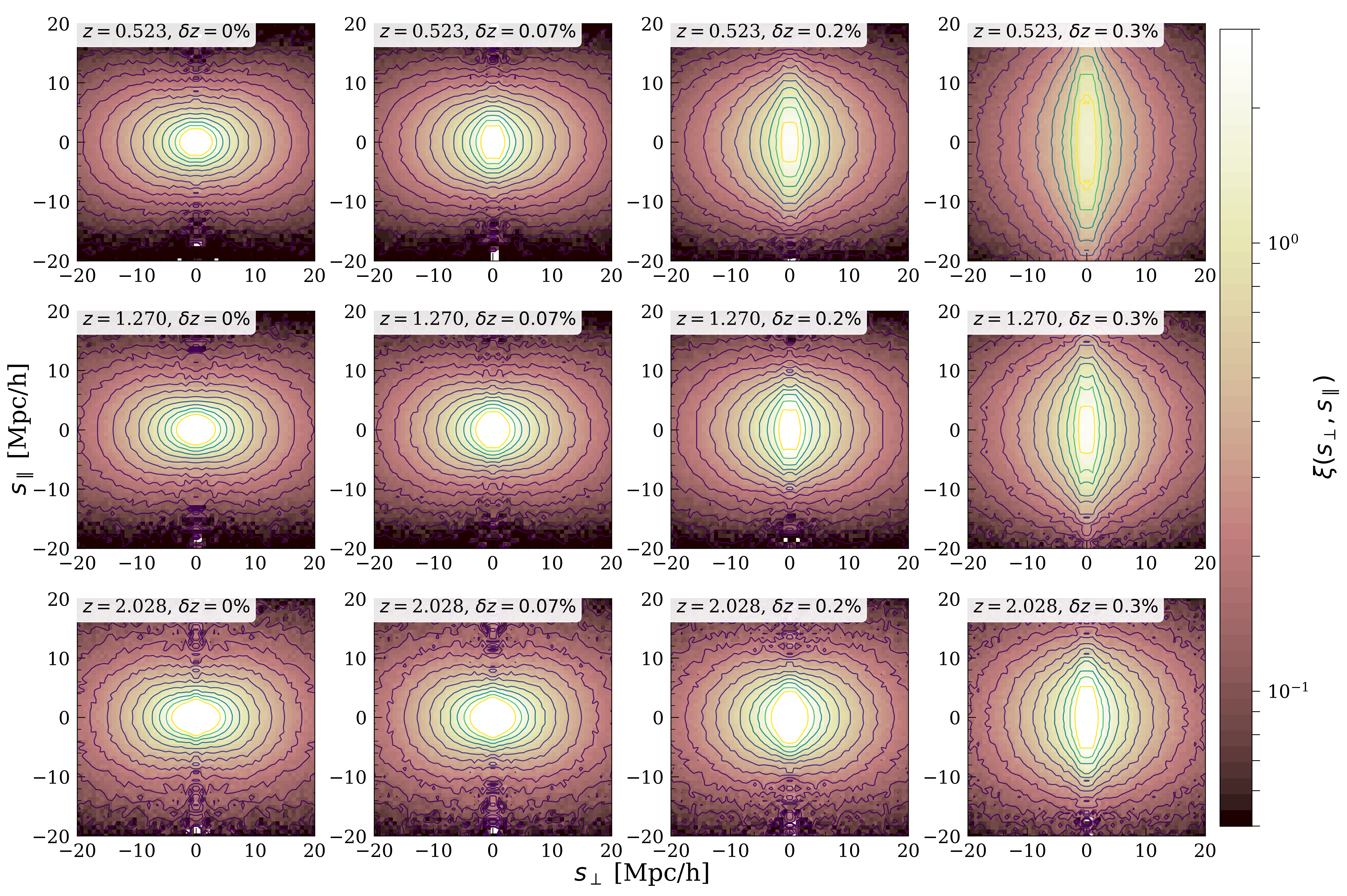
Figure 4: Iso-correlation contours of $\xi(s_{\perp},s_{\parallel})$, at the three redshifts indicated by the labels, in correspondence of the correlation levels $\xi(s_{\perp},s_{\parallel})$ $={0.05,\leavevmode\nobreak\ 0.07,\leavevmode\nobreak\ 0.09,\leavevmode\nobreak\ 0.13,\leavevmode\nobreak\ 0.18,\leavevmode\nobreak\ 0.24,\leavevmode\nobreak\ 0.33,\leavevmode\nobreak\ 0.45,\leavevmode\nobreak\ 0.62,\leavevmode\nobreak\ 0.85,\leavevmode\nobreak\ 1.17,\leavevmode\nobreak\ 1.6,\leavevmode\nobreak\ 2.2,\leavevmode\nobreak\ 3}$. The panels refer to different redshifts (rows) and different amplitudes of the redshift errors (columns), as indicated by the labels. The colour bar on the right side indicates the amplitude of $\xi(s_{\perp},s_{\parallel})$ .

Figure 4 shows the 2PCF as a function of the transverse, $s_{\perp}$, and parallel, $s_{\parallel}$, separations to the LOS, at three different redshifts. The iso-correlation contours of $\xi(s_{\perp},s_{\parallel})$ are measured in the range $[0.05,\leavevmode\nobreak\ 3]$, for different values of the redshift measurement errors, $\delta z$. As it can be seen, redshift errors introduce spurious clustering anisotropies at small scales, enhancing the clustering signal along the LOS, analogously to the effect due to Fingers-of-God (FoG) (Marulli et al., 2012b).

As described in Section 3.1, it is convenient to project the two-dimensional 2PCF, $\xi(s_{\perp},s_{\parallel})$, onto one-dimensional statistics, such as the multipole moments and the clustering wedges. In Figs. 5 and 6 we show the redshift-space monopole and quadrupole moments, and the redshift-space radial and transverse wedges, respectively. In agreement with Marulli et al. (2012b), we find a progressive suppression of the slope of the 2PCF monopole, tending to flatness for increasingly larger redshift errors (e.g Sereno et al., 2015). On the other hand, the quadrupole signal increases. The results for the clustering wedges are similar, showing a small-scale suppression in the transverse wedge, when the redshift errors are included, while the radial wedge increases. As shown in Fig. 4 and discussed in details in the next Sections, the spurious anisotropies caused by redshift errors in the multipole moments and wedges have a scale-dependent pattern similar to the FoG one, caused by small-scale incoherent motions.

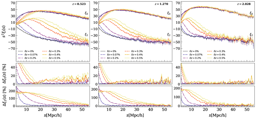
Figure 5: Redshift-space 2PCF monopole, $\xi_{0}$, and quadrupole, $\xi_{2}$, of the MDPL2 DM haloes, at three different redshifts. The lines correspond to the 2PCFs measured in mock catalogues with different redshift errors, as indicated by the labels. The bottom subpanels show the relative percentage differences with respect to the case with no redshift errors.

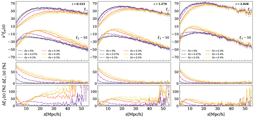
Figure 6: As Fig. 5, but for the redshift-space 2PCF perpendicular, $\xi_{\perp}$, and parallel, $\xi_{\parallel}$, wedges of the MDPL2 DM haloes. For clarity, $\xi_{\parallel}$ is shifted by $-50$.

Alternative statistics that can be used to quantify the impact of redshift errors in the clustering pattern are the ratio between the redshift-space and real-space monopole, $R(s)$, and the ratio between the redshift-space quadrupole and monopole, $Q(s)$. In the linear regime, these quantities can be written as follows:

$$R(s) = \frac{\xi_{0}(s)}{\xi_{0}(r)}=1+\frac{2\beta}{3}+\frac{\beta^{2}}{5},$$ (11)

$$Q(s) = \frac{\xi_{2}(s)}{\xi_{0}(s)-\frac{3}{s^{3}}\int^{s}_{0}ds^{\prime}\xi(s^{\prime})s^{\prime 2}}=\frac{\frac{4}{3}\beta+\frac{4}{7}\beta^{2}}{1+\frac{2\beta}{3}+\frac{\beta^{2}}{5}}\,,$$ (12)

where $\xi_{0}$ and $\xi_{2}$ are the redshift-space monopole and quadrupole of the 2PCF, respectively, and $\beta$ is the linear distortion parameter defined as $\beta\equiv f(z)/b(z)$, with $f(z)$ being the linear growth rate. Figure 7 shows the measured $R(s)$ and $Q(s)$ statistics, as a function of redshift errors, compared to the theoretical predictions derived by assuming the Tinker et al. (2008, 2010) effective bias. As it can be seen, we find a good agreement between measurements and theoretical predictions in the case without redshift errors, for both estimators, at large enough scales (beyond $\sim 10$$h^{-1}\,\mbox{Mpc}$). Redshift errors introduce scale-dependent distortions in both these statistics. In particular, their effect is to increase (decrease) the $R(s)$ ratio above (below) a characteristic scale, whereas the $Q(s)$ is reduced, especially at small scales.

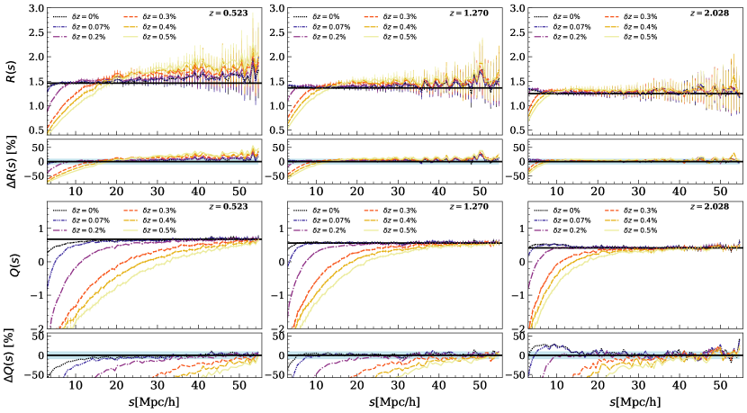
Figure 7: The ratio between the redshift-space and real-space monopole moments, $R(s)$ (upper panels), and between the redshift-space quadrupole and monopole, $Q(s)$ (lower panels), at three different redshifts (different columns) and for different redshift errors, as indicated by the labels. Horizontal lines represent the theoretical predictions obtained assuming the Tinker et al. (2008, 2010) effective bias. The error bars are computed by propagating the 2PCF bootstrap errors and the subpanels show the relative percentage differences with respect to the case with no redshift errors.

4 Modelling redshift-space distortions

In this Section, we describe the models used to parameterise the RSD in the 2PCF multipoles and wedges. Then we derive constraints on $f\sigma_{8}$ and $b\sigma_{8}$ parameters for each mock catalogue constructed from the MDPL2 simulations, investigating the effect of possible redshift errors. The multipole moments are modelled as follows:

$$\xi_{l}(s)=i^{l}\int_{-\infty}^{\infty}\frac{\mbox{d}k}{2\pi^{2}}k^{2}P_{l}(k)j_{l}(ks)\,,$$ (13)

where $j_{l}$ are the spherical Bessel functions, and $P_{l}(k)$ are the power spectrum multipoles:

$$P_{l}(k)=\frac{2l+1}{2}\int_{-1}^{1}\mbox{d}\mu\,P^{s}(k,\mu)L_{l}(\mu)\,.$$ (14)

We consider three widely-used RSD models to estimate the redshift-space 2D power spectrum $P^{s}(k,\mu)$:

• Dispersion model (Peacock & Dodds, 1996):

  $$P^{s}(k,\mu)=D(k,f,\mu,\sigma_{12})\,\left(1+\frac{f}{b}\mu^{2}\right)^{2}\,b^{2}\,P_{\delta\delta}(k)\,,$$ (15)

  where the second term on the right-hand side of the equation describes the distortions caused by the large-scale coherent peculiar motions (Kaiser, 1987), $P_{\delta\delta}(k)$ is the matter power spectrum, and $D(k,f,\mu,\sigma_{12})$ is a damping factor that characterises the incoherent peculiar motions at small scales. In this work, we consider both the Gaussian and the Lorentzian forms of the damping factor, as already done in previous works (see e.g. Scoccimarro, 2004; Taruya et al., 2010; Marulli et al., 2012b; Xu et al., 2012, 2013; Zheng et al., 2017):

  $$D(k,f,\mu,\sigma_{12})=\begin{cases}\exp\left[-k^{2}f^{2}\mu^{2}\sigma_{12}^{2}\right],&\text{ Gaussian,}\\ \frac{1}{(1+k^{2}f^{2}\mu^{2}\sigma_{12}^{2})},&\text{Lorentzian.}\end{cases}$$ (16)

• Scoccimarro model (Scoccimarro, 2004): this model considers the density and velocity divergence fields separately to account for their non-linear mode coupling:

  $$P^{s}(k,\mu)=D(k,f,\mu,\sigma_{12})\left(b^{2}P_{\delta\delta}(k)+2fb\mu^{2}P_{\delta\theta}(k)+\right.\\ \left.+f^{2}\mu^{4}P_{\theta\theta}(k)\right)\,,$$ (17)

  where $P_{\delta\theta}$ and $P_{\theta\theta}$ are the density-velocity divergence cross-spectrum and the velocity divergence auto-spectrum, respectively. In the linear regime, both $P_{\delta\theta}$ and $P_{\theta\theta}$ tend to $P_{\delta\delta}$.

• TNS model (Taruya et al., 2010): besides taking into account the non-linear mode coupling between the density and velocity divergence fields, this model introduces also additional terms to correct for systematics at small scales:

  $$P^{s}(k,\mu)=D(k,f,\mu,\sigma_{12})\biggl{(}b^{2}P_{\delta\delta}(k)+2fb\mu^{2}P_{\delta\theta}(k)+\\ +f^{2}\mu^{4}P_{\theta\theta}(k)+C_{A}(k,\mu,f,b)+C_{B}(k,\mu,f,b)\biggr{)}\,.$$ (18)

  Following Taruya et al. (2010) and de la Torre & Guzzo (2012), we express the correction terms of the TNS model derived from the Standard Perturbation Theory (SPT), $C_{A}$ and $C_{B}$, in terms of the basic statistics of density $\delta$ and velocity divergence $\theta(\mathbf{k})\equiv[-i\mathbf{k}\cdot\mathbf{v}(\mathbf{k})]/[af(a)H(a)]$. Specifically, they can be written as follows:

  $$\begin{split}C_{A}(k,\mu)&=(k\mu f)\int\frac{d^{3}\boldsymbol{p}}{(2\pi)^{3}}\frac{p_{z}}{p^{2}}\\ &\times\left[B_{\sigma}(\boldsymbol{p},\boldsymbol{k}-\boldsymbol{p},-\boldsymbol{k})-B_{\sigma}(\boldsymbol{p},\boldsymbol{k},-\boldsymbol{k}-\boldsymbol{p})\right]\,,\end{split}$$ (19)

  $$C_{B}(k,\mu) =(k\mu f)^{2}\int\frac{d^{3}\boldsymbol{p}}{(2\pi)^{3}}F(\boldsymbol{p})F(\boldsymbol{k}-\boldsymbol{p})\,,$$ (20)

  with

  $$F(\boldsymbol{p}) =\frac{p_{z}}{p^{2}}\left[P_{\delta\theta}(p)+f\frac{p_{z}^{2}}{p^{2}}P_{\theta\theta}(p)\right]\,,$$ (21)

  and $B_{\sigma}$ being the cross-bispectrum. The $C_{A}$ and $C_{B}$ terms are proportional to $b^{3}$ and $b^{4}$, respectively, and can be re-written as a power series expansion of $b$, $f$ and $\mu$, and their respective contributions to the total power spectrum. For a detailed explanation on the perturbation theory calculations of these correction terms, see Appendix A of Taruya et al. (2010), while for what concerns the correlation function and the dependence of the spatial bias of the considered tracers, see Appendix A of de la Torre & Guzzo (2012).

The $P_{\delta\delta}$, $P_{\delta\theta}$ and $P_{\theta\theta}$ terms can be computed directly from perturbation theory (Eulerian, Lagrangian or Time renormalisation) or, alternatively, using fitting formulae (see e.g. Jennings, 2012; Pezzotta et al., 2017; Bel et al., 2019). In this paper we adopt the former approach, estimating the terms of the total power spectrum using the SPT, which consists of expanding the statistics of interest as a sum of infinite terms, each one corresponding to a $n$-loop correction (see e.g. Gil-Marín et al., 2012). In particular, we consider corrections up to $1$-loop order, thus the power spectrum can be written as follows:

$$P^{\mathrm{SPT}}(k)=P^{(0)}(k)+P^{(1)}(k)=P^{(0)}(k)+2P_{13}(k)+P_{22}(k)\,,$$ (22)

where the 0-loop correction term, $P^{(0)}(k)$, corresponds to the linear power spectrum and the one-loop contribution, $P^{(1)}(k)$, consists of the sum of two terms, $P_{13}(k)$ and $P_{22}(k)$. To estimate the power spectrum at $z>0$, we rescale Eq. (22) by the linear growth factor, $D(z)$, as follows: $P_{xy}(k,z)=[D(z)/D(0)]^{2}P_{11}(k)+[D(z)/D(0)]^{4}[P_{22}(k)+2P_{13}(k)]$, where ${x,y}$ is either $\delta$ or $\theta$ (for details on these terms see e.g. Bernardeau et al., 2002; Gil-Marín et al., 2012). We compute the quantities in Eq. (22) with the CPT Library .

We exploit a full Markov Chain Monte Carlo (MCMC) statistical analysis to estimate posterior distribution constraints on the three free RSD model parameters $\left[f\sigma_{8},\,b\sigma_{8},\,\sigma_{12}\right]$. We consider a standard Gaussian likelihood, defined as follows:

$$-2\ln\mathcal{L}=\sum_{i,j=1}^{N}\left[\xi_{k}^{D}(s_{i})-\xi_{k}^{M}(s_{i})\right]C_{k}^{-1}(s_{i},s_{j})\left[\xi_{k}^{D}(s_{j})-\xi_{k}^{M}(s_{j})\right]\,,$$ (23)

with $N$ being the number of bins at which the multipole moments and the wedges are computed, and the superscripts $D$ and $M$ referring to data and model, respectively.

We perform the MCMC analysis on all the MDPL2 mock halo catalogues to get the global evolution of the constrained parameters. First we compare the constraints on $f\sigma_{8}$, $b\sigma_{8}$ and $\sigma_{12}$ at $z=1.032$, obtained with the Gaussian and Lorentzian damping factors. The results are shown in Fig. 8 for the redshift-space multipole moments and clustering wedges. As it can be appreciated, the systematic errors are lower when the damping factor is modelled with a Gaussian function, as expected since redshifts errors are modelled as Gaussian variables and their effects are captured by the damping term in the models, in agreement with Marulli et al. (2012b). Thus, in the following we will adopt the Gaussian form. The fluctuations in the results are not statistically significant, but deserve further investigations with higher resolution simulations.

Figures 9 and 10 show the measured multipole moments and the clustering wedges compared to best-fit model predictions for the dispersion, Scoccimarro and TNS models, at $z=0.523,\leavevmode\nobreak\ 1.032,\leavevmode\nobreak\ 2.028$, and for different redshift measurement errors. We find good agreement between the best-fit models and the measured statistics on scales down to about 10$h^{-1}\,\mbox{Mpc}$, for both multipole moments and clustering wedges, also when we include redshift errors in the measurements. Overall, the dispersion model is the one that deviates the most at small scales, especially when multipole moments are considered, whereas the two SPT-based models considered in this work fit the data better, in both statistics. In particular, at scales larger than 10$h^{-1}\,\mbox{Mpc}$, the percentage differences between the TNS model and the measurements are lower than about $3\%$ and $5\%$ for the monopole and the quadrupole, respectively. While they are lower than about $3\%$ and $7\%$ for the perpendicular wedge and the parallel wedge, respectively.

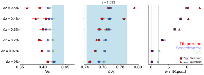
Figure 8: Best-fit constraints on [$f\sigma_{8}$, $b\sigma_{8}$, $\sigma_{12}$] of the MDPL2 mock catalogue at $z=1.032$, assuming the Gaussian and Lorentzian form of the damping factor for different values of redshift errors. The dispersion, Scoccimarro and TNS models are differentiated by colour, as labelled, and the error bars show the $68\%$ marginalised posterior uncertainties. The vertical lines show the theoretical predictions – the linear growth rate is computed as $f=\Omega_{M}(z)^{\gamma}$; the bias, $b$, is computed by assuming the Tinker et al. (2008, 2010) effective bias model; the prediction for $\sigma_{12}$ is obtained from the MCMC analysis with only $\sigma_{12}$ as free parameter, while all the other parameters are fixed at their theoretical values. Upper panel: results from the redshift-space monopole and quadrupole moments; lower panel: results from the perpendicular and parallel wedges.

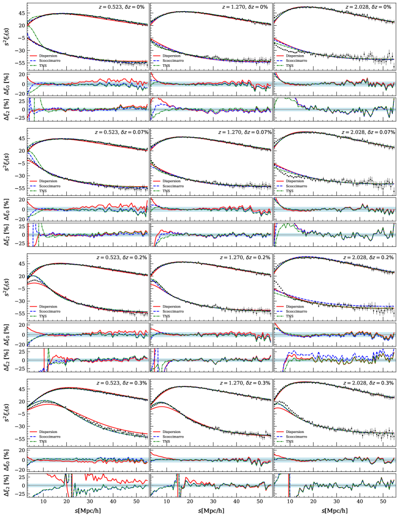
Figure 9: Redshift-space monopole, $\xi_{0}$, and quadrupole, $\xi_{2}$, moments of the MDPL2 mock catalogues, compared to the best-fit models – dispersion model (red solid), Scoccimarro model (dashed blue) and TNS model (dash-dotted green). The results are shown at three different redshifts (different columns), and for different measurement redshift errors (different rows), as indicated by the labels. The subpanels show the relative percentage differences with respect to the measurements.

Figure 10: As Fig. 9 but for the redshift-space perpendicular, $\xi_{\perp}$, and parallel, $\xi_{\parallel}$, wedges of the MDPL2 mock catalogues.

The marginalised posterior constraints on the parameters $\left[f\sigma_{8},\,b\sigma_{8},\,\sigma_{12}\right]$, as a function of redshift, are reported in Figs. 11 and 12, for multipole moments and clustering wedges, respectively. The solid black lines represent the theoretical predictions. In particular, $b\sigma_{8}$ is computed assuming the Tinker et al. (2008, 2010) effective bias model, while the pairwise velocity dispersion, $\sigma_{12}$, corresponds to the best-fit value obtained when the remaining parameters are fixed to the theoretical expectations.

In the case with no redshift errors, we find a systematic bias in the $f\sigma_{8}$ constraints of about $10\%$ at low redshifts, $z<1$, for the dispersion model, in agreement with previous works (e.g. Bianchi et al., 2012; Marulli et al., 2012b; Marulli et al., 2017). The Scoccimarro and TNS model provide more accurate constraints, with a systematic bias of about $8\%$ and $5\%$, respectively. At high redshifts, $z\geq 1$, the agreement between $f\sigma_{8}$ measurements and the expected values improves. In particular, the Scoccimarro model recovers $f\sigma_{8}$ within $4\%$, while the TNS model within $3\%$. The constraints on $b\sigma_{8}$ are overall in good agreement for all models, being the TNS model the one with the lowest deviation with respect to the theoretical expectations, which is found to be less than $2\%$ at all redshifts considered.

As we have seen in Fig. 4, the spurious anisotropies caused by Gaussian redshift errors are similar to the FoG distortions. The combined effects of redshift errors and FoG are thus parameterised by the single damping term of the RSD models. Indeed, as shown in Figs. 11 and 12, the estimated value of the $\sigma_{12}$ parameter of the damping term systematically increases as redshift errors increase. At $z\geq 1$, the $f\sigma_{8}$ and $b\sigma_{8}$ constraints are not significantly affected by the introduction of Gaussian redshift errors, up to $\delta z=0.5\%$. On the other hand, at lower redshifts the impact is more significant, at all redshift errors considered.

Figures 13 and 14 summarise our main results, showing the marginalised posterior constraints at $68\%$ confidence level for $f\sigma_{8}$, $b\sigma_{8}$ and $\sigma_{12}$, obtained from the MCMC analysis of the redshift-space monopole and quadrupole moments, and of the perpendicular and parallel clustering wedges, respectively. Moreover, Figs. 13 and 14 compare the results obtained by fitting the 2PCF statistics in the comoving scale range $10<r[$$h^{-1}\,\mbox{Mpc}$$]<55$ to the ones obtained at scales $r>30$ $h^{-1}\,\mbox{Mpc}$. As expected, while the statistical uncertainties are larger in the latter scale, the systematic discrepancies are slightly reduced. In particular, the discrepancies of the TNS model on both the growth rate and the linear bias are reduced below $3\%$, at $z<1.5$, for redshift errors up to $\delta z\sim 0.3\%$. On the other hand, at larger redshifts it seems more convenient to consider in the analysis also the small scales, which can be reliably described by all the RSD models considered.

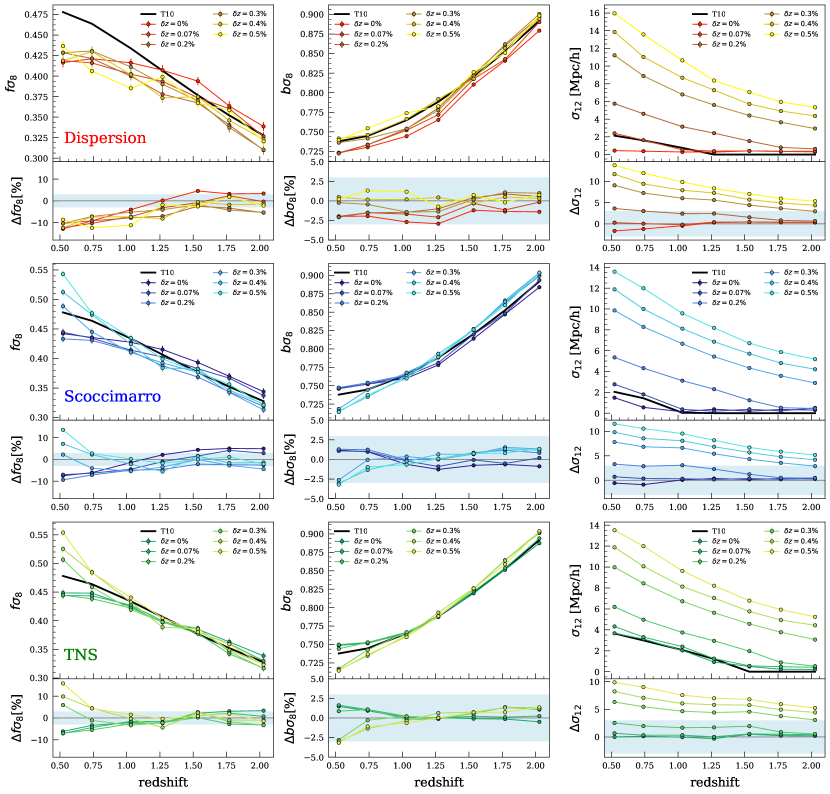
Figure 11: Best-fit constraints on [$f\sigma_{8}$, $b\sigma_{8}$, $\sigma_{12}$] obtained from the redshift-space monopole and quadrupole moments, as a function of redshift (different columns), and for different values of redshift errors, as indicated by the labels. The error bars show the $68\%$ marginalised posterior uncertainties. The black solid lines show the theoretical predictions – the linear growth rate is computed as $f=\Omega_{M}(z)^{\gamma}$; the bias, $b$, is computed by assuming the Tinker et al. (2008, 2010) effective bias model; the prediction for $\sigma_{12}$ is obtained from the MCMC analysis with only $\sigma_{12}$ as free parameter, while all the other parameters are fixed at their theoretical values. Upper panels: dispersion model; central panels: Scocimarro model; lower panel: TNS model. The subpanels show the relative percentage differences with respect to the theoretical prediction.

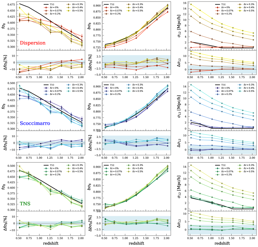
Figure 12: The same as Fig. 11, but using perpendicular and parallel clustering wedges.

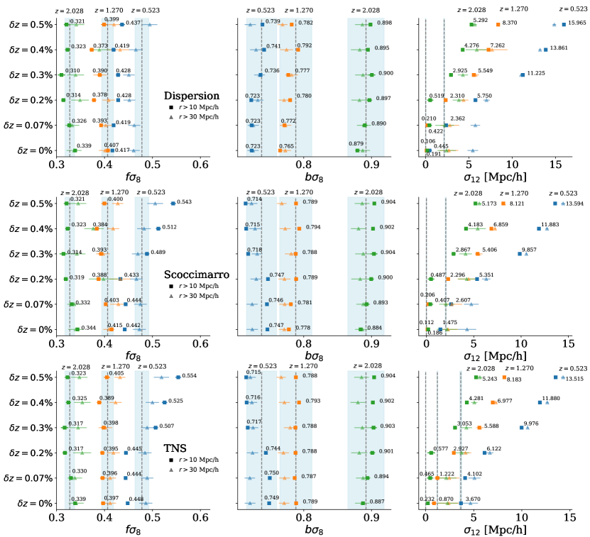
Figure 13: Marginalised posterior constraints at $68\%$ confidence level for $f\sigma_{8}$ (first column), $b\sigma_{8}$ (central column) and $\sigma_{12}$ (last column), obtained from the MCMC analysis of the redshift-space monopole and quadrupole moments. The results are shown at three different redshifts as labelled $z=0.523$, $z=1.270$ and $z=2.028$, for the dispersion model (first row), the Scoccimarro model (central row), and the TNS model (bottom row), as labelled. The vertical black lines are centred on theoretical expectations, with the shaded area reporting the $3\%$ region, for comparison.

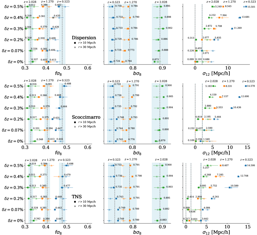
Figure 14: As Fig. 13, but using the redshift-space perpendicular, $\xi_{\perp}$, and parallel, $\xi_{\parallel}$, clustering wedges.

5 Conclusions

We presented a systematic analysis of state-of-the-art statistical methods to infer cosmological constraints on the linear growth rate from RSD in the 2PCF. This work follows from the analyses presented in Bianchi et al. (2012) and Marulli et al. (2012b); Marulli et al. (2017). The two main improvements of the current study with respect to the latter are that i) we considered both the monopole and quadrupole moments of the 2PCF, as well as the perpendicular and parallel clustering wedges, and ii) we compared three RSD models, that is the dispersion model, the Scoccimarro model and the TNS model, investigating the impact of Gaussian redshift errors on the linear growth rate and bias constraints. The analysis has been performed in the redshift range $0.5\lesssim z\lesssim 2$, and in the comoving scale range $10<r[$$h^{-1}\,\mbox{Mpc}$$]<55$.

The main results of this analysis can be summarised as follows:

• At $z<1$, the linear growth rate measured with the dispersion model is underestimated by about $10\%$, in agreement with previous findings; the Scoccimarro and TNS models provide slightly better constraints, with a systematic bias of about $8\%$ and $5\%$, respectively.

• As expected, limiting the analysis at $r>30$ $h^{-1}\,\mbox{Mpc}$, the statistical uncertainties become larger, while the systematic discrepancies are slightly reduced. In particular, the systematics of the TNS model on both the growth rate and the linear bias are reduced below $3\%$, at $z<1.5$, for redshift errors up to $\delta z\sim 0.3\%$.

• At $z\geq 1$, all the RSD models considered provide constraints in good agreement with expectations. The TNS model is the one which performs better, with growth rate uncertainties below about $3\%$.

• Gaussian redshift errors introduce spurious anisotropies, whose effect combines with the one of the small-scale incoherent motions responsible of the FoG distortions. This effect is captured by the damping factor of the RSD model considered, and can be marginalised over in the statistical analysis, not introducing statistically significant bias in the RSD constraints, especially at $z\geq 1$.

Overall, we find that the TNS model is the best one among the RSD models considered, in agreement with previous analyses (e.g. Pezzotta et al., 2017). The linear growth rate can be recovered within about $3\%$ of accuracy in the redshift range $1<z<2$, typical of next generation galaxy survey missions, like Euclid (Laureijs et al., 2011), even in the presence of Gaussian redshift errors up to $\delta z=0.5\%$, which are greater than those expected from forthcoming spectroscopic galaxy surveys (see Table 1). Though this accuracy is good enough for clustering analyses in current redshift surveys, the RSD models have to be further improved not to introduce significant systematics in RSD constraints from next generation galaxy surveys, which aim at mapping the cosmic structure growth rate with statistical uncertainties below few percent. Moreover, the mass resolution of the N-body simulations considered in this work is too low to model the DM haloes typically hosting the faintest galaxies that will be detected in next-generation surveys. As the systematic model uncertainties are expected to be larger for lower bias tracers, the performances of the considered RSD models on forthcoming clustering measurements could be even worse than the ones reported here. Higher resolution simulations are required to investigate this issue and provide more realistic forecasts on systematic uncertainties.

References

- Achitouv et al. (2017) Achitouv I., Blake C., Carter P., Koda J., Beutler F., 2017, Phys. Rev. D, 95, 083502
- Adams & Blake (2017) Adams C., Blake C., 2017, MNRAS, 471, 839
- Alam et al. (2017) Alam S., et al., 2017, MNRAS, 470, 2617
- Amendola et al. (2018) Amendola L., et al., 2018, Living Reviews in Relativity, 21, 2
- Barrow et al. (1984) Barrow J. D., Bhavsar S. P., Sonoda D. H., 1984, MNRAS, 210, 19P
- Bel et al. (2019) Bel J., Pezzotta A., Carbone C., Sefusatti E., Guzzo L., 2019, A&A, 622, A109
- Bennett et al. (2013) Bennett C. L., et al., 2013, ApJS, 208, 20
- Bernardeau et al. (2002) Bernardeau F., Colombi S., Gaztañaga E., Scoccimarro R., 2002, Phys. Rep., 367, 1
- Beutler et al. (2012) Beutler F., et al., 2012, MNRAS, 423, 3430
- Beutler et al. (2014) Beutler F., et al., 2014, MNRAS, 443, 1065
- Bianchi et al. (2012) Bianchi D., Guzzo L., Branchini E., Majerotto E., de la Torre S., Marulli F., Moscardini L., Angulo R. E., 2012, MNRAS, 427, 2420
- Blake et al. (2012) Blake C., et al., 2012, MNRAS, 425, 405
- Blake et al. (2013) Blake C., et al., 2013, MNRAS, 436, 3089
- Campbell et al. (2014) Campbell L. A., et al., 2014, MNRAS, 443, 1231
- Chuang & Wang (2013) Chuang C.-H., Wang Y., 2013, MNRAS, 435, 255
- Chuang et al. (2013) Chuang C.-H., et al., 2013, MNRAS, 433, 3559
- Chuang et al. (2016) Chuang C.-H., et al., 2016, MNRAS, 461, 3781
- Costa et al. (2017) Costa A. A., Xu X.-D., Wang B., Abdalla E., 2017, Journal of Cosmology and Astro-Particle Physics, 2017, 028
- DES Collaboration et al. (2017) DES Collaboration et al., 2017, ArXiv e-prints: 1708.01530,
- Davis & Peebles (1983) Davis M., Peebles P. J. E., 1983, ApJ, 267, 465
- Davis et al. (2011) Davis M., Nusser A., Masters K. L., Springob C., Huchra J. P., Lemson G., 2011, MNRAS, 413, 2906
- Efron (1979) Efron B., 1979, Ann. Statist., 7, 1
- Feix et al. (2015) Feix M., Nusser A., Branchini E., 2015, Phys. Rev. Lett., 115, 011301
- García-Farieta et al. (2019) García-Farieta J. E., Marulli F., Veropalumbo A., Moscardini L., Casas-Miranda R. A., Giocoli C., Baldi M., 2019, MNRAS, 488, 1987
- Gil-Marín et al. (2012) Gil-Marín H., Wagner C., Verde L., Porciani C., Jimenez R., 2012, Journal of Cosmology and Astro-Particle Physics, 2012, 029
- Granett et al. (2019) Granett B. R., Favole G., Montero-Dorta A. D., Branchini E., Guzzo L., de la Torre S., 2019, arXiv e-prints, p. arXiv:1905.10375
- Guzzo et al. (2000) Guzzo L., et al., 2000, A&A, 355, 1
- Guzzo et al. (2014) Guzzo L., et al., 2014, A&A, 566, A108
- Hamaus et al. (2016) Hamaus N., Pisani A., Sutter P. M., Lavaux G., Escoffier S., Wand elt B. D., Weller J., 2016, Phys. Rev. Lett., 117, 091302
- Hamilton (1998) Hamilton A. J. S., 1998, Linear Redshift Distortions: A Review. Springer Netherlands, Dordrecht, pp 185–275
- Hartlap et al. (2007) Hartlap J., Simon P., Schneider P., 2007, A&A, 464, 399
- Hawken et al. (2017) Hawken A. J., et al., 2017, A&A, 607, A54
- Howlett et al. (2015) Howlett C., Ross A. J., Samushia L., Percival W. J., Manera M., 2015, MNRAS, 449, 848
- Huterer et al. (2017) Huterer D., Shafer D. L., Scolnic D. M., Schmidt F., 2017, J. Cosmology Astropart. Phys., 2017, 015
- Ivezic et al. (2008) Ivezic Z., et al., 2008, ArXiv e-prints: 0805.2366,
- Jackson (1972) Jackson J. C., 1972, Monthly Notices of the Royal Astronomical Society, 156, 1P
- Jennings (2012) Jennings E., 2012, MNRAS, 427, L25
- Kaiser (1987) Kaiser N., 1987, MNRAS, 227, 1
- Kazin et al. (2012) Kazin E. A., Sánchez A. G., Blanton M. R., 2012, MNRAS, 419, 3223
- Klypin et al. (2016) Klypin A., Yepes G., Gottlöber S., Prada F., Heß S., 2016, MNRAS, 457, 4340
- Knebe et al. (2011) Knebe A., et al., 2011, MNRAS, 415, 2293
- Landy & Szalay (1993) Landy S. D., Szalay A. S., 1993, ApJ, 412, 64
- Laureijs et al. (2011) Laureijs R., et al., 2011, arXiv e-prints, p. arXiv:1110.3193
- Lewis et al. (2000) Lewis A., Challinor A., Lasenby A., 2000, The Astrophysical Journal, 538, 473
- Ling et al. (1986) Ling E. N., Frenk C. S., Barrow J. D., 1986, MNRAS, 223, 21P
- Maartens et al. (2015) Maartens R., Abdalla F. B., Jarvis M., Santos M. G., SKA Cosmology SWG f. t., 2015, arXiv e-prints, p. arXiv:1501.04076
- Marulli et al. (2011) Marulli F., Carbone C., Viel M., Moscardini L., Cimatti A., 2011, MNRAS, 418, 346
- Marulli et al. (2012a) Marulli F., Baldi M., Moscardini L., 2012a, MNRAS, 420, 2377
- Marulli et al. (2012b) Marulli F., Bianchi D., Branchini E., Guzzo L., Moscardini L., Angulo R. E., 2012b, MNRAS, 426, 2566
- Marulli et al. (2016) Marulli F., Veropalumbo A., Moresco M., 2016, Astronomy and Computing, 14, 35
- Marulli et al. (2017) Marulli F., Veropalumbo A., Moscardini L., Cimatti A., Dolag K., 2017, A&A, 599, A106
- Marulli et al. (2018) Marulli F., et al., 2018, A&A, 620, A1
- Merloni et al. (2012) Merloni A., et al., 2012, ArXiv e-prints: 1209.3114,
- Mohammad et al. (2018) Mohammad F. G., et al., 2018, A&A, 610, A59
- Moresco & Marulli (2017) Moresco M., Marulli F., 2017, MNRAS, 471, L82
- Ntampaka et al. (2019) Ntampaka M., Rines K., Trac H., 2019, arXiv e-prints, p. arXiv:1906.07729
- Okumura et al. (2016) Okumura T., et al., 2016, PASJ, 68, 38
- Pacaud et al. (2018) Pacaud F., et al., 2018, A&A, 620, A10
- Parkinson et al. (2012) Parkinson D., et al., 2012, Phys. Rev. D, 86, 103518
- Peacock & Dodds (1996) Peacock J. A., Dodds S. J., 1996, MNRAS, 280, L19
- Percival et al. (2004) Percival W. J., et al., 2004, MNRAS, 353, 1201
- Pezzotta et al. (2017) Pezzotta A., et al., 2017, A&A, 604, A33
- Planck Collaboration et al. (2014) Planck Collaboration et al., 2014, A&A, 571, A16
- Planck Collaboration et al. (2016) Planck Collaboration et al., 2016, A&A, 594, A13
- Planck Collaboration et al. (2018) Planck Collaboration et al., 2018, arXiv e-prints, p. arXiv:1807.06205
- Reid et al. (2012) Reid B. A., et al., 2012, MNRAS, 426, 2719
- Riebe et al. (2013) Riebe K., et al., 2013, Astronomische Nachrichten, 334, 691
- Rodríguez-Puebla et al. (2016) Rodríguez-Puebla A., Behroozi P., Primack J., Klypin A., Lee C., Hellinger D., 2016, MNRAS, 462, 893
- Samushia et al. (2012) Samushia L., Percival W. J., Raccanelli A., 2012, MNRAS, 420, 2102
- Samushia et al. (2014) Samushia L., et al., 2014, MNRAS, 439, 3504
- Sánchez et al. (2013) Sánchez A. G., et al., 2013, MNRAS, 433, 1202
- Sánchez et al. (2014) Sánchez A. G., et al., 2014, MNRAS, 440, 2692
- Sánchez et al. (2017) Sánchez A. G., et al., 2017, MNRAS, 464, 1640
- Santos et al. (2015) Santos M., et al., 2015, in Advancing Astrophysics with the Square Kilometre Array (AASKA14). p. 19 (arXiv:1501.03989)
- Scoccimarro (2004) Scoccimarro R., 2004, Phys. Rev. D, 70, 083007
- Sereno et al. (2015) Sereno M., Veropalumbo A., Marulli F., Covone G., Moscardini L., Cimatti A., 2015, MNRAS, 449, 4147
- Silk (2017) Silk J., 2017, in 14th International Symposium on Nuclei in the Cosmos (NIC2016). p. 010101 (arXiv:1611.09846), doi:10.7566/JPSCP.14.010101
- Smith et al. (2003) Smith R. E., et al., 2003, Monthly Notices of the Royal Astronomical Society, 341, 1311
- Spergel et al. (2013) Spergel D., et al., 2013, ArXiv e-prints: 1305.5422,
- Takahashi et al. (2012) Takahashi R., Sato M., Nishimichi T., Taruya A., Oguri M., 2012, ApJ, 761, 152
- Taruya et al. (2010) Taruya A., Nishimichi T., Saito S., 2010, Phys. Rev. D, 82, 063522
- Tinker et al. (2008) Tinker J., Kravtsov A. V., Klypin A., Abazajian K., Warren M., Yepes G., Gottlöber S., Holz D. E., 2008, ApJ, 688, 709
- Tinker et al. (2010) Tinker J. L., Robertson B. E., Kravtsov A. V., Klypin A., Warren M. S., Yepes G., Gottlöber S., 2010, ApJ, 724, 878
- Tojeiro et al. (2012) Tojeiro R., et al., 2012, MNRAS, 424, 2339
- Topping et al. (2018) Topping M. W., Shapley A. E., Steidel C. C., Naoz S., Primack J. R., 2018, ApJ, 852, 134
- Upadhye (2019) Upadhye A., 2019, Journal of Cosmology and Astro-Particle Physics, 2019, 041
- Vega-Ferrero et al. (2017) Vega-Ferrero J., Yepes G., Gottlöber S., 2017, MNRAS, 467, 3226
- Wang et al. (2018) Wang Y., et al., 2018, ApJ, 868, 130
- Wright et al. (2019) Wright B. S., Koyama K., Winther H. A., Zhao G.-B., 2019, Journal of Cosmology and Astro-Particle Physics, 2019, 040
- Xu et al. (2012) Xu X., Padmanabhan N., Eisenstein D. J., Mehta K. T., Cuesta A. J., 2012, Monthly Notices of the Royal Astronomical Society, 427, 2146
- Xu et al. (2013) Xu X., Cuesta A. J., Padmanabhan N., Eisenstein D. J., McBride C. K., 2013, Monthly Notices of the Royal Astronomical Society, 431, 2834
- Zandanel et al. (2018) Zandanel F., Fornasa M., Prada F., Reiprich T. H., Pacaud F., Klypin A., 2018, MNRAS, 480, 987
- Zheng et al. (2017) Zheng Y., Zhang P., Oh M., 2017, Journal of Cosmology and Astro-Particle Physics, 2017, 030
- de la Torre & Guzzo (2012) de la Torre S., Guzzo L., 2012, MNRAS, 427, 327
- de la Torre et al. (2013) de la Torre S., et al., 2013, A&A, 557, A54
- de la Torre et al. (2017) de la Torre S., et al., 2017, A&A, 608, A44
- van den Bosch & Jiang (2016) van den Bosch F. C., Jiang F., 2016, MNRAS, 458, 2870