Deep Learning based Precoding for the
MIMO Gaussian Wiretap Channel

Abstract

A novel precoding method based on supervised deep neural networks is introduced for the multiple-input multiple-output Gaussian wiretap channel. The proposed deep learning (DL)-based precoding learns the input covariance matrix through offline training over a large set of input channels and their corresponding covariance matrices for efficient, reliable, and secure transmission of information. Furthermore, by spending time in offline training, this method remarkably reduces the computation complexity in real-time applications. Compared to traditional precoding methods, the proposed DL-based precoding is significantly faster and reaches near-capacity secrecy rates. DL-based precoding is also more robust than transitional precoding approaches to the number of antennas at the eavesdropper. This new approach to precoding is promising in applications in which delay and complexity are critical.

I introduction

Wiretap channel [1, 2] is a three-node network, consisting of a transmitter, a legitimate receiver, and an eavesdropper, in which encoding is designed to transmit the legitimate receiver’s message securely and reliably. This model, which lays the foundation of physical layer security, is then extended to multi-antenna nodes. The capacity of multiple-input multiple-output (MIMO) Gaussian wiretap channel under an average power constraint is established in [3, 4, 5]. This capacity expression is abstracted as a non-convex optimization problem over the covariance matrix of the input signal. This problem is fundamental in the study of physical layer security in the MIMO settings and thus has attracted extensive research in the past decade and has been explored in different ways. Despite this, the closed-form covariance matrix is known only in some special cases [6, 7, 8], and optimal signaling to achieve the capacity is still unknown, in general.

There are several sub-optimal and iterative solutions for this problem. Generalized singular value decomposition (GSVD)-based precoding, which splits the transmit channel into several parallel subchannels, provides a closed-form solution [3, 9]. This closed-form solution is, however, far from capacity in some antenna settings, e.g., when the legitimate receiver has a single antenna [8]. Alternating optimization and water filling (AO-WF) algorithm [10] is another well-known solution which converts the non-convex problem to a convex problem and solves it in an iterative manner. However, the complexity of this method is high and the solution is not stable under certain antenna settings [11]. Recently, a new parameterization of the covariance matrix was proposed for two-antenna transmitters and its optimal closed-form solution was obtained in [8]. This method is then extended to arbitrary antennas in [11]. Although the new reformulation of the problem based on the rotation matrices is optimal, the way to find the parameters is iterative and time-consuming, especially for large number of transmit antennas. Overall, despite extensive research and fundamental importance of this problem, the existing signaling methods, except for closed-form solutions, suffer either from a high computational complexity or performance loss.

Motivate by the above shortcomings and recent successful applications of deep learning (DL) in communication over the physical layer [12], in this work, we exploit DL for a secure and reliable signaling design in the MIMO Gaussian wiretap channel. DL is a new emerging sub-field of machine learning (ML), and similar to ML, provides a data-driven approach to tackle traditionally challenging problems [13]. It holds promise for performance improvements in complex scenarios that are difficult to describe with tractable mathematical models or solutions. While DL prevails in computer vision, speech and audio processing, and natural language processing, its introduction to communication systems is relatively new. Nonetheless, DL is increasingly being used to solve communication problems in the physical layer. Particularly, DL is being applied to typically hard and intractable problems such as encoding and decoding schemes, beamforming, and power allocation in MIMO, etc. [14, 12, 15, 16, 17].

Recent research efforts have shown that DL is useful in many sophisticated communications problems. In [12], a neural network (NN)-based autoencoder is proposed for end-to-end reconstruction and communication system design. Although the above work is limited to a differentiable channel, [18] shows that it is possible for autoencoders to work well over the air. Supervised reinforcement learning is proposed to characterize communication architecture with a mathematical channel model absence in [19]. In a more relevant paper to our work, [20] proposes learning encoding and decoding schemes by NN to realize confidential message transmission over the Gaussian wiretap channel. These successful examples applying DL to communication systems mainly exploit the classification ability of the DL.

In this paper, we develop a DL-based precoding using a residual network [21] to reliably and securely transmit information over the MIMO wiretap channel with near-capacity rates. With multiple hidden and intermediate layers of neurons, the proposed DL-based precoding can effectively characterize the precoding matrix. Multiple hidden layers and non-linearity properties of the deep neural networks (DNN), enables the proposed DL-based precoding to learn sophisticated mapping between inputs (channel matrices) and output (covariance matrix). Via offline training, the proposed DL-based precoding learns from a large number of near-optimal covariance matrices and performs well in fitting, regressing and predicting precoding and power allocation matrices. Once trained well, the network achieves a near-capacity secure rate very quickly and with a little memory. Hence, this approach is promising to be applied into Internet of things (IoT), which intrinsically have limited computation abilities and battery life.

The performance of the proposed precoding, in terms of complexity and achievable rate, is compared with the exiting analytical and numerical solutions, namely, GSVD and AO-WF. It is shown that similar or better performance can be achieved significantly faster. Moreover, unlike existing solutions, the proposed DL-based precoding is robust to the change in the number of antennas at the eavesdropper. This is meaningful progress towards secure communication in a more practical setting in which the number of antennas at the eavesdropper is unknown.

The remainder of this paper is organized as follows. In Section II, the system model of the MIMO wiretap channel is described. In Section III, a novel DNN is designed to learn the input covariance matrix. The training phase and experimental results are discussed in Section IV, and the paper is concluded in Section V.

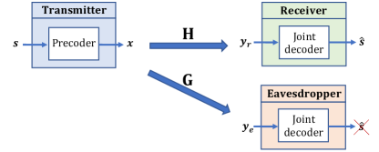
Figure 1: The MIMO wiretap channel.

II System Model

The MIMO wiretap channel is a model for reliable and secure communication over the air which includes a transmitter equipped with $n_{t}$ antennas which sends a message to a legitimate receiver with $n_{r}$ antennas while keeping it confidential from an eavesdropper equipped with $n_{e}$ antennas. The system model is shown in Fig. 1 in which $\mathbf{s}\in\mathbb{R}^{n_{t}}$ is the information vector, $\mathbf{x}\in\mathbb{R}^{n_{t}}$ is the transmitted signal, $\mathbf{y}_{r}\in\mathbb{R}^{n_{r}}$ and $\mathbf{y}_{e}\in\mathbb{R}^{n_{e}}$ are the received signal at receiver and eavesdropper sides. The received signals at the legitimate receiver and the eavesdropper sides at time $m$ can be, respectively, expressed as

$$\mathbf{y}_{r}[m]=\mathbf{H}\mathbf{x}[m]+\mathbf{w}_{r}[m],$$ (1a)

$$\mathbf{y}_{e}[m]=\mathbf{G}\mathbf{x}[m]+\mathbf{w}_{e}[m],$$ (1b)

in which $\mathbf{H}\in\mathbb{R}^{n_{r}\times n_{t}}$ and $\mathbf{G}\in\mathbb{R}^{n_{e}\times n_{t}}$ are the channel matrices corresponding to the receiver and eavesdropper, $\mathbf{w_{r}}\in\mathbb{R}^{n_{r}}$ and $\mathbf{w_{e}}\in\mathbb{R}^{n_{e}}$ are Gaussian white noises with zero means and identity covariance matrices. The channel input is subject to an average total power constraint [5], i.e.,

$$||\mathbf{x}||^{2}=\frac{1}{M}\sum_{m=0}^{M-1}(\mathbf{x}[m]^{T}\mathbf{x}[m])\leq P,$$ (2)

where $M$ is the length of $\mathbf{x}$. The capacity expression of the MIMO wiretap channel (1) under the average power (2) is expressed as [5]

$$\mathcal{C}_{s}= \max\limits_{\mathbf{Q}}\frac{1}{2}\log|\mathbf{I}_{n_{r}}+\mathbf{HQH}^{T}|-\frac{1}{2}\log|\mathbf{I}_{n_{e}}+\mathbf{GQG}^{T}|,$$

$$\;\;\mathrm{s.t.}\quad\mathbf{Q}\succeq 0,\textmd{tr}(\mathbf{Q})\leq P,$$ (3)

in which the covariance matrix $\mathbf{Q}=E\{\mathbf{xx}^{T}\}\in\mathbb{R}^{n_{t}\times n_{t}}$ is symmetric and positive semi-definite, and $\mathbf{A}^{T}$, $\textmd{tr}(\mathbf{A})$, and $|\mathbf{A}|$ represent transpose, trace, and determinant of matrix $\mathbf{A}$, respectively.

Optimal closed-form $\mathbf{Q}$ is known only for special numbers of antenna settings [11]. There, however, are a few well-known sub-optimal analytical and numerical solutions for arbitrary numbers of antennas. Among them are GSVD, AO-WF, and rotation-based precoding, as discussed earlier. We note that since eigenvalue decomposition of $\mathbf{Q}$ results in $\mathbf{Q}=\mathbf{V}\mathbf{\Lambda}\mathbf{V}^{t}$, we can design the transmitted signal vector as

$$\mathbf{x}=\mathbf{V}\mathbf{\Lambda}^{\frac{1}{2}}\mathbf{s},$$ (4)

in which

• $\mathbf{V}$ is the precoding matrix,

• $\mathbf{\Lambda}^{\frac{1}{2}}$ is the power allocation matrix, and

• $\mathbf{s}$ is the information signal vector with covariance $\mathbf{I}$.

Thus, knowing the covariance matrix is equivalent to knowing the corresponding precoding and power allocation matrices. Hence, these two are used equivalently in this paper.

III Deep Learning Architecture for Precoding

This paper designs a precoder based on a DNN for the MIMO Gaussian wiretap channel. The inputs of the network are channel matrices $(\mathbf{H}$ and $\mathbf{G})$ and their non-linear combinations. The output is the upper triangular part of the optimal covariance matrix $\mathbf{Q}$. After the training process, the network learns the features of optimal covariance matrix $\mathbf{Q}$ over different channels. In this paper, $\mathbf{Q}$ used for training is obtained from AO-WF method and is called optimal $\mathbf{Q}$. In fact, the network tries to learn how to get a $\mathbf{Q}$ similar to that of AO-WF. Alternatively, rotation-based method [11] can be used.

III-A Input Features

For $n_{t}=2$, optimal $\mathbf{Q}$ is known analytically from [8]. Here we consider $n_{t}=3$ in this paper. The network input vector $\mathbf{v}$ contains 72 features as shown in Fig. 2. These features include the elements of channel matrices, i.e., $\mathbf{H}$ and $\mathbf{G}$, and their non-linear combinations as shown in Fig. 2. Note that sing Sylvester’s determinant identity the arguments of the logarithms in (II) can be written as

$$\left|\mathbf{I}_{n_{r}}+\mathbf{H}\mathbf{Q}\mathbf{H}^{T}\right|=\left|\mathbf{I}_{n_{t}}+\mathbf{H}^{T}\mathbf{H}\mathbf{Q}\right|,$$ (5a)

$$\left|\mathbf{I}_{n_{e}}+\mathbf{G}\mathbf{Q}\mathbf{G}^{T}\right|=\left|\mathbf{I}_{n_{t}}+\mathbf{G}^{T}\mathbf{G}\mathbf{Q}\right|.$$ (5b)

Hence, $\mathbf{H}^{T}\mathbf{H}$ or $\mathbf{G}^{T}\mathbf{G}$ can be considered as a whole which are both $n_{t}\times n_{t}$ matrices. In this paper, the input vector $\mathbf{v}$ is designed as

$$\mathbf{v}\triangleq[0.05\mathbf{v}_{1},0.002\mathbf{v}_{2},0.0001\mathbf{v}_{3}]^{T},$$ (6)

in which $\mathbf{v}_{1}$, $\mathbf{v}_{2}$, and $\mathbf{v}_{3}$ are defined as

$$\mathbf{v}_{1}\triangleq{\rm vec}([\mathbf{H}^{T}\mathbf{H}\;\;\mathbf{G}^{T}\mathbf{G}]),$$ (7a)

$$\mathbf{v}_{2}\triangleq{\rm vec}([\mathbf{H}^{T}\mathbf{H}\;\;\mathbf{G}^{T}\mathbf{G}]^{T}[\mathbf{H}^{T}\mathbf{H}\;\;\mathbf{G}^{T}\mathbf{G}]),$$ (7b)

$$\mathbf{v}_{3}\triangleq{\rm cube}(\mathbf{v}_{1}),$$ (7c)

where ${\rm vec}(\cdot)$ is the vectorization of a matrix and ${\rm cube}(\cdot)$ is the element-wise cube operation. The coefficients of these vectors are used for normalization and weighting. The sketch of the input vector is shown in Fig. 2. Here, $\mathbf{v}_{1}$ can be seen as an original feature whereas $\mathbf{v}_{2}$ and $\mathbf{v}_{3}$ provide additional nonlinear combination of the original features which increases the probability that DNN can learn the mapping from input to desired output.

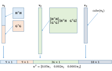
Figure 2: The input design.

III-B Network Design

The network architecture for $n_{t}=3$ is shown in Fig. 3. This is a fully-connected neural network (FCNN) with parametric rectified linear units (PReLUs) [22] as activation functions. FCNN can be seen as a special convolutional neural network with filter size $1\times 1$ [23]. PReLU can provide more trainable parameters and prevent over-fitting[22]. Besides, we introduce a few shortcut connections proposed in the residual network [24]. The shortcut connections are able to reduce the difficulty of training process and make the network converge better. We add a PReLU layer with unique trainable parameters to each shortcut connection.

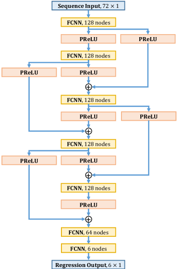
Figure 3: The proposed DL architecture.

III-C Expected Output

The covariance matrix for $n_{t}=3$ is given by

$$\mathbf{Q}=\left[\begin{array}[]{ccc}q_{11}&q_{12}&q_{13}\\ q_{12}&q_{22}&q_{23}\\ q_{13}&q_{23}&q_{33}\end{array}\right].$$ (11)

The output vector $\mathbf{q}$ contains the upper triangular part of the covariance matrix $\mathbf{Q}$ since it is symmetry. More specifically,

$$\mathbf{q}\triangleq[q_{11},q_{22},q_{33},q_{12},q_{23},q_{13}]^{T}.$$ (12)

Each $\mathbf{Q}$ is given by AO-WF [10]. The network is required to learn the relation between the channels and $\mathbf{Q}$.

IV Training Procedure and Simulation Results

The training procedure and regression results are demonstrated in this section. We also examine the performance of DL-based precoding in this section.

IV-A Data Set Generation

The experiments are associated with three training sets, i.e., TrainingSet-I, TrainingSet-II and TrainingSet-III, as shown in Table I. TrainingSet-I and TrainingSet-II contain $2,000,000$ samples. Each sample contains $72$ input features contributed by the channel matrices. The channels are generated randomly following the standard Gaussian distribution. TrainingSet-I is for $n_{t}=3$, $n_{r}=4$, and $n_{e}=3$ whereas in TrainingSet-II the number of antennas are $n_{t}=3$, $n_{r}=2$, and $n_{e}=1$.

TABLE I: Details of the Data Sets.

	$n_{t}$	$n_{r}$	$n_{e}$	number of samples
TrainingSet-I	3	2	1	2,000,000
TestSet-I	3	2	1	1000
TrainingSet-II	3	4	3	2,000,000
TestSet-II	3	4	3	1000
TrainingSet-III	Cascade of TrainingSet-I and TrainingSet-II
TestSet-III	Cascade of TestSet-I and TestSet-II

Then, AO-WF [10] is used to generate optimal $\mathbf{Q}$ for each set of channels and the total average transmit power constraint is $P\leq 20W$ for all cases. The upper triangular part of $\mathbf{Q}$ is the output used for supervised learning. TrainingSet-III is the cascade of TrainingSet-I and TrainingSet-II with random order of samples. We also generate TestSet-I and TestSet-II as test data sets, each of which having $1000$ samples with antenna setting corresponding to TrainingSet-I and TrainingSet-II.

IV-B Training Process

In the training process, the proposed DL-based precoding is trained three times using TrainingSet-I, TrainingSet-II and TrainingSet-III. The training process is executed on a single graph card (NVIDA GeForce GTX 1080) and Adam[25] is used as the optimization method. Except for the batch size, all training process has the same hyper-parameters. The total epochs are $4,000,000$. Learning rate is initially set $0.001$ and then is decreased $20\%$ after every $80$ epochs. The batch size for TrainingSet-I and TrainingSet-II is $2000$ whereas for TrainingSet-III it is $4000$. Considering the number of samples in TrainingSet-III is twice as many as that in TrainingSet-I and TrainingSet-II, the doubled batch size will ensure the training time consumption for all training process was approximately the same; it was about $20$ hours in our experiments.

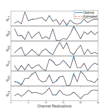
Figure 4: Comparison between optimal and estimated elements in $\mathbf{Q}$ when $n_{t}=3$, $n_{r}=2$, and $n_{e}=1$.

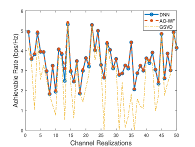
(a) TrainingSet-I with TestSet-I

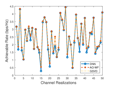
(b) TrainingSet-II with TestSet-II

Figure 5: Comparison of achievable secrecy rate using corresponding training and test sets.

IV-C Performance of the DL-based Precoding

The performance of the proposed DL-based precoding can be evaluated by corresponding training and test data sets, i.e., TrainingSet-I with TestSet-I and TrainingSet-II with TestSet-II. The mean squared error (MSE) for evaluating $\mathbf{Q}$ is shown in Table II. Besides, Fig. 4 illustrates the estimation results and their expected values for TestSet-I. It is seen that the elements in $\mathbf{Q}$ are estimated with fairly good MSEs.

Once the network “learns” to estimate the optimal $\mathbf{Q}$, it is ready to be used for precoding and power allocation based on (4). The achievable rate versus channel realizations is shown in Figs. 5(a) and 5(b), and is compared with those of AO-WF and GSVD. Further, the average secrecy rate of each test process is provided in Table III.

TABLE II: MSE of DL-based Precoding with Corresponding Training and Test Data Sets.

Training Data Set	TrainingSet-I	TrainingSet-II
Test Data Set	TestSet-I	TestSet-II
MSE of $\hat{q}_{11}$	0.1402	0.0779
MSE of $\hat{q}_{22}$	0.1338	0.0740
MSE of $\hat{q}_{33}$	0.1479	0.0633
MSE of $\hat{q}_{12}$	0.1167	0.0770
MSE of $\hat{q}_{23}$	0.1425	0.0741
MSE of $\hat{q}_{13}$	0.1220	0.0711

TABLE III: Average Achievable Secrecy Rate.

Training Set	Test Set	DL-based	AO-WF	GSVD
TrainingSet-I	TestSet-I	3.3980	3.4741	2.5197
TrainingSet-II	TestSet-II	2.3381	2.4827	2.4639
TrainingSet-III	TestSet-I	3.3947	3.4741	2.5197
TrainingSet-III	TestSet-II	2.3267	2.4827	2.4639

As can be seen from the figures, the proposed DL-based precoding is able to reach a secrecy rate comparable to that of AO-WF. Besides, the proposed DL-based precoding performs better than GSVD in the case $n_{t}=3$, $n_{r}=2$, and $n_{e}=1$. More importantly, as illustrated in Table IV, the proposed DL-based precoding is much more efficient than the traditional methods. Although DL’s training time is long, the training process is usually realized offline. Accordingly, a well-trained precoding is a promising tool in the Gaussian MIMO wiretap problem especially for IoT devices with limited energy and computing power.

TABLE IV: Average Time for One Realization.

	DL-based	AO-WF	GSVD
Time Cost (ms)	0.0255	243	0.513

IV-D Cascading Training Sets

If we exchange the test and training data sets in previous simulation, i.e., if we use TrainingSet-II with TestSet-I and TrainingSet-I with TestSet-II, the DL-based precoding cannot estimate $\mathbf{Q}$ very well as shown in Table V. This problem can be solved by cascading the two training sets as a new one, named TrainingSet-III. From Table VI, it is seen that the performance becomes much better and reaches a similar level when training separately without additional training epochs by doubling the batch size, as mentioned in Subsection IV-B. The secrecy rates for this case are shown in Figs. 6(a) and 6(b). The average achievable rate is further shown in the last two rows of Table III. It is seen that the proposed DL architecture is able to learn from existing optimal results with different $n_{r}$ and $n_{e}$ if it is trained with such samples. Overall, the DL-based precoding can achieve secrecy rate more efficiently than traditional iterative methods.

TABLE V: MSE of DL-based Precoding with Opposite
Training and Test Data Sets.

Training Data Set	TrainingSet-II	TrainingSet-I
Test Data Set	TestSet-I	TestSet-II
MSE of $\hat{q}_{11}$	2.8353	7.4462
MSE of $\hat{q}_{22}$	2.8124	7.7543
MSE of $\hat{q}_{33}$	3.0579	6.8545
MSE of $\hat{q}_{12}$	2.7646	5.4432
MSE of $\hat{q}_{23}$	2.3103	4.4098
MSE of $\hat{q}_{13}$	2.1800	5.0406

TABLE VI: MSE of DL-based Precoding with Cascaded Training Sets.

Training Data Set	TrainingSet-III
Test Data Set	TestSet-I	TestSet-II
MSE of $\hat{q}_{11}$	0.1313	0.1564
MSE of $\hat{q}_{22}$	0.1234	0.1386
MSE of $\hat{q}_{33}$	0.1219	0.1364
MSE of $\hat{q}_{12}$	0.1526	0.1351
MSE of $\hat{q}_{23}$	0.1057	0.1596
MSE of $\hat{q}_{13}$	0.1384	0.1123

IV-E Applying a Deeper Network

The performance of DL-based precoding can be further improved by increasing the depth of the NN. The network architecture in Fig. 3 (denoted as DeepNet) contains $7$ FCNN layers, $9$ PReLU activation layers, $4$ shortcut connections, and $4$ addition nodes. If we add anther $4$ FCNN layers and repeat the shortcut connections, a deeper network named as DeeperNet can be obtained. The DeeperNet contains $7$ FCNN layers, $17$ PReLU activation layers, $8$ shortcut connections, and $8$ addition nodes. The average achievable secrecy rates using different data sets are compared in Table VII. The secrecy rate obtained by the DeeperNet outperforms that of the DeepNet. However, since the depth of the network is doubled, the time consumption is increased to $0.0405{\rm ms}$ per channel realization, i.e., it takes two times the DeepNet. Therefore, the proposed DeepNet compromises between secrecy performance and time cost.

TABLE VII: Average of Achievable Secrecy Rate.

Training Set	Test Set	DeepNet	DeeperNet	AO-WF
TrainingSet-I	TestSet-I	3.3980	3.4215	3.4741
TrainingSet-II	TestSet-II	2.3381	2.4137	2.4827

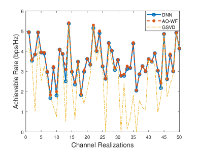
(a) TrainingSet-III with TestSet-I

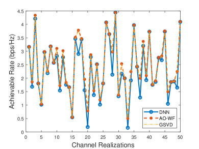
(b) TrainingSet-III with TestSet-II

Figure 6: Comparison of achievable secrecy rate using combined training set and separate test sets.

V Conclusions

In this paper, a DL-based precoding has been proposed for the MIMO Gaussian wiretap channel. The input features of the DL-based precoding are generated by channel matrices and the output have the elements of the covariance matrix. The network is build up with FCNN, residual connections, and PReLU. The experiments show that the proposed precoding is much faster than existing methods and achieves a reasonable and stable secrecy performance. The method is energy-saving and much less complex which makes it a promising approach to physical layer security of IoT networks.

One practical issue in the context of the wiretap channel is that the number of antennas at the eavesdropper is assumed known. This work makes meaningful progress toward eliminating or, at least, being less dependent on this assumption.

References

- [1] A. D. Wyner, “The wire-tap channel,” Bell system technical journal, vol. 54, no. 8, pp. 1355–1387, 1975.
- [2] I. Csiszár and J. Korner, “Broadcast channels with confidential messages,” IEEE Transactions on Information Theory, vol. 24, no. 3, pp. 339–348, 1978.
- [3] A. Khisti and G. W. Wornell, “Secure transmission with multiple antennas—part II: The MIMOME wiretap channel,” IEEE Transactions on Information Theory, vol. 11, no. 56, pp. 5515–5532, 2010.
- [4] F. Oggier and B. Hassibi, “The secrecy capacity of the MIMO wiretap channel,” IEEE Transactions on Information Theory, vol. 57, no. 8, pp. 4961–4972, 2011.
- [5] T. Liu and S. Shamai, “A note on the secrecy capacity of the multiple-antenna wiretap channel,” IEEE Transactions on Information Theory, vol. 55, no. 6, pp. 2547–2553, 2009.
- [6] S. A. A. Fakoorian and A. L. Swindlehurst, “Full rank solutions for the MIMO Gaussian wiretap channel with an average power constraint,” IEEE Transactions on Signal Processing, vol. 61, no. 10, pp. 2620–2631, 2013.
- [7] P. Parada and R. Blahut, “Secrecy capacity of SIMO and slow fading channels,” in Proceedings of IEEE International Symposium on Information Theory (ISIT), pp. 2152–2155, 2005.
- [8] M. Vaezi, W. Shin, and H. V. Poor, “Optimal beamforming for Gaussian MIMO wiretap channels with two transmit antennas,” IEEE Transactions on Wireless Communications, vol. 16, no. 10, pp. 6726–6735, 2017.
- [9] S. A. A. Fakoorian and A. L. Swindlehurst, “Optimal power allocation for GSVD-based beamforming in the MIMO Gaussian wiretap channel,” in Proceedings of IEEE International Symposium on Information Theory (ISIT), pp. 2321–2325, 2012.
- [10] Q. Li, M. Hong, H.-T. Wai, Y.-F. Liu, W.-K. Ma, and Z.-Q. Luo, “Transmit solutions for MIMO wiretap channels using alternating optimization,” IEEE Journal on Selected Areas in Communications, vol. 31, no. 9, pp. 1714–1727, 2013.
- [11] X. Zhang, Y. Qi, and M. Vaezi, “A rotation-based method for precoding in Gaussian MIMOME channels,” arXiv preprint arXiv:1908.00994, 2019.
- [12] T. O’Shea and J. Hoydis, “An introduction to deep learning for the physical layer,” IEEE Transactions on Cognitive Communications and Networking, vol. 3, no. 4, pp. 563–575, 2017.
- [13] L. Deng and D. Yu, “Deep learning: Mthods and applications,” Foundations and Trends in Signal Processing, vol. 7, no. 3–4, pp. 197–387, 2014.
- [14] A. Zappone, M. Di Renzo, and M. Debbah, “Wireless networks design in the era of deep learning: Model-based, AI-based, or both?,” arXiv preprint arXiv:1902.02647, 2019.
- [15] C. Zhang, P. Patras, and H. Haddadi, “Deep learning in mobile and wireless networking: A survey,” IEEE Communications Surveys & Tutorials, 2019.
- [16] M. Vaezi, G. Amarasuriya, Y. Liu, A. Arafa, F. Fang, and Z. Ding, “Interplay between NOMA and other emerging technologies: A survey,” arXiv preprint arXiv:1903.10489, 2019.
- [17] K.-L. Besser, C. R. Janda, P.-H. Lin, and E. A. Jorswieck, “Flexible design of finite blocklength wiretap codes by autoencoders,” in Proceedings of IEEE International Conference on Acoustics, Speech and Signal Processing (ICASSP), pp. 2512–2516, 2019.
- [18] S. Dörner, S. Cammerer, J. Hoydis, and S. ten Brink, “Deep learning based communication over the air,” IEEE Journal of Selected Topics in Signal Processing, vol. 12, no. 1, pp. 132–143, 2017.
- [19] F. A. Aoudia and J. Hoydis, “End-to-end learning of communications systems without a channel model,” in Proceedings of IEEE Conference on Signals, Systems, and Computers, pp. 298–303, 2018.
- [20] R. Fritschek, R. F. Schaefer, and G. Wunder, “Deep learning for the Gaussian wiretap channel,” arXiv preprint arXiv:1810.12655, 2018.
- [21] Y. LeCun, Y. Bengio, and G. Hinton, “Deep learning,” nature, vol. 521, no. 7553, p. 436, 2015.
- [22] K. He, X. Zhang, S. Ren, and J. Sun, “Delving deep into rectifiers: Surpassing human-level performance on imagenet classification,” in Proceedings of the IEEE International Conference on Computer Vision, pp. 1026–1034, 2015.
- [23] J. Long, E. Shelhamer, and T. Darrell, “Fully convolutional networks for semantic segmentation,” in Proceedings of IEEE Conference on Computer Vision and Pattern Recognition (CVPR), pp. 3431–3440, 2015.
- [24] K. He, X. Zhang, S. Ren, and J. Sun, “Deep residual learning for image recognition,” in Proceedings of IEEE Conference on Computer Vision and Pattern Recognition (ICCV), pp. 770–778, 2016.
- [25] D. P. Kingma and J. Ba, “Adam: A method for stochastic optimization,” arXiv preprint arXiv:1412.6980, 2014.