A new scalable algorithm for computational optimal control under uncertainty

Abstract

We address the design and synthesis of optimal control strategies for high-dimensional stochastic dynamical systems. Such systems may be deterministic nonlinear systems evolving from random initial states, or systems driven by random parameters or processes. The objective is to provide a validated new computational capability for optimal control which will be achieved more efficiently than current state-of-the-art methods. The new framework utilizes direct single or multi-shooting discretization, and is based on efficient vectorized gradient computation with adaptable memory management. The algorithm is demonstrated to be scalable to high dimensional nonlinear control systems with random initial condition and unknown parameters.

1 Introduction

Designing optimal control strategies for high-dimensional stochastic dynamical systems is critical in many engineering applications, such as search of unknown targets with autonomous vehicles, path planning of heterogeneous agents, and quantum control [6, 12, 29, 11, 31]. Such systems may be modeled as nonlinear control systems of the form

$$\dot{\bm{x}}=\bm{f}(\bm{x},\bm{u}),\qquad\bm{x}(0)=\bm{x}_{0}(\omega),\qquad t\in[0,t_{f}],$$ (1)

where $\bm{x}(t)\in\mathbb{R}^{n}$ is the system’s state (random process), $\bm{u}(t)\in\mathbb{R}^{m}$ is the (deterministic) control, and $\bm{x}_{0}(\omega)\in\mathbb{R}^{n}$ is an random initial condition with prescribed probability density function $p_{0}(\bm{x})$. As is well known [25, 24, 22], uncertain parameters in $\bm{f}$ can always be transferred to the initial condition. The solution to the Cauchy problem (1) is a function of the initial state $\bm{x}_{0}$ and a functional of the control $\bm{u}(t)$, i.e., $\bm{x}(t)=\bm{x}(t,\bm{x}_{0},[\bm{u}])$. We aim at designing $\bm{u}(t)$ by solving the optimal control problem

$$\begin{cases}\displaystyle\min_{\bm{u}(t)}J([\bm{x}(t)],[\bm{u}(t)])\vspace{0.1cm}\\ \quad\text{subject to:}\\ \begin{array}[]{ll}\qquad\dot{\bm{x}}=\bm{f}(\bm{x},\bm{u}),&\bm{x}(0)=\bm{x}_{0}(\omega)\quad\text{($\bm{x}_{0}$ random)}\\ \qquad\bm{g}(\bm{u}(t))\leq\bm{0},&\textrm{(constraints on the control)}\\ \qquad\bm{h}\left(\mathbb{E}\{\bm{x}(t)\}\right)\leq\bm{0},&\textrm{(ensemble path constraints)}\end{array}\end{cases}$$ (2)

where $J([\bm{x}(t)],[\bm{u}(t)])$ is a cost functional [21] that involves an expectation $\mathbb{E}\{\cdot\}$ over the probability distribution of the initial state $\bm{x}_{0}(\omega)$. For example, $J$ could be of the form

$$J([\bm{x}(t)],[\bm{u}(t)])=\mathbb{E}\{F(\bm{x}(t_{f}))\}+\int_{0}^{t_{f}}r(\bm{u}(\tau))d\tau,$$ (3)

where $F(\bm{x})$ and $r(\bm{u})$ are smooth functions. Other examples of $J$ involve the probability of detecting an unknown target [12], measures of risk [17], or indicator functions of disease propagation in a network of interacting individuals [10]. The optimal control problem (2) is, in general, a high-dimensional (large-scale) non-convex optimization problem. State-of-the-art algorithms to solve such problem are largely based on sampling the random initial state $\bm{x}_{0}$, e.g., using Gauss quadrature [12, 16] or Monte Carlo methods [4, 13, 23], and then computing a large ensemble of trajectories corresponding to a particular control $\bm{u}(t)$. With such ensemble of paths available, one can then evaluate the performance metric $J$ by approximating the expectation operator with an appropriate cubature rule [12, 13, 28, 30], and close the optimal control loop with a suitable optimizer (see Figure 1). The formulation of optimal control strategies based on sample trajectories is straightforward, and it yields an optimal control problem which can be solved by classical algorithms, e.g., pseudospectral methods [5, 7, 8]. However, such algorithms are computationally intensive, and they are not effective even in a moderate number of state variables for the following reasons: First, the set of sample trajectories can propagate in phase space in a very complicated manner. This implies that a large number of paths is usually required to evaluate the performance metric. Secondly, as the number of sample paths increases, the dimension of the discretized optimal control problem rapidly becomes intractable. In particular, for a dynamical system with $n$ state variables and $M$ sample paths, the nonlinear control problem has dimension $nM$ ($M$ copies of the $n$-dimensional dynamical system at each iteration of the optimizer). This is one of the main bottlenecks that limits the applicability of probabilistic collocation methods to systems with low dimensional random input vectors. For systems with large number of random variables, the memory requirements and computational cost becomes unacceptably large.

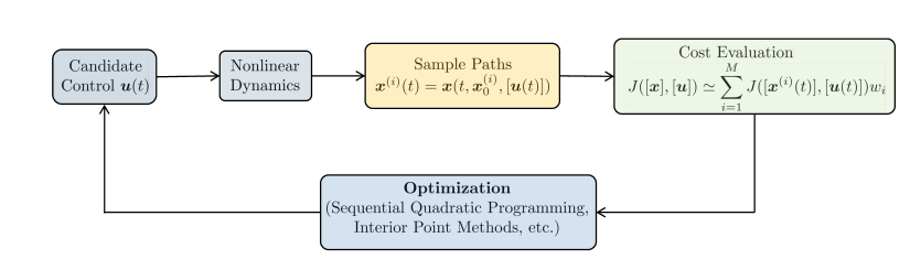
Figure 1: Sketch of the proposed data-driven optimal control architecture. The new control algorithm is based on interior point optimization methods, common sub-expression elimination, and exact gradient information obtained with automatic differentiation and computational graphs.

In this paper, we aim at overcoming these limitations by developing a new algorithm for computational optimal control under uncertainty that is applicable to high-dimensional stochastic dynamical systems, and engineering control applications requiring online (real-time) implementations. The new algorithm is based on interior point optimization methods [26, 3], common sub-expression elimination, and exact gradients obtained via automatic differentiation and computational graphs [1, 2]. They key features of the proposed algorithm are:

1. Multi-shooting optimal control schemes: Multi-shooting is known for its numerical stability in solving deterministic optimal control problems. Based on piece-wise constant (in time) control approximation, we modified the deterministic algorithm and made it effective for uncertain optimal control problems. This includes imposing particle-independent continuity conditions across adjacent time segments.

2. Accurate gradient computations: The optimization solver we developed combines an interior point method [26, 3, 32] which converges most efficiently using accurate gradient calculations over the controlled ensemble. In this work we compare a number of established techniques for gradient computation, namely traditional operator overloading algorithmic differentiation (ADOLC) [27], more modern graph based methods for gradient calculation (TensorFlow) [1] and the most commonly used finite differences approach. We demonstrate that graph based methods offer precision with considerable speed improvement over more traditional algorithms, albeit at the expense of considerable memory utilization, and slowness in initialization.

3. Efficient memory utilization: The algorithm has extremely low memory requirements, which means that it allows us to process a massive number of sample trajectories (in parallel) and determine the performance metric and associated optimal controls in a very efficient way. To achieve these results we developed a common sub-expression elimination (CSE) technique that can substantially reduce memory consumption during computations. As we shall see in section 3.2, CSE considerably reduces the growth of memory requirements with respect to the increase of the time discretization points in multi-shooting. This feature is essential for solving high dimensional problems and problems with long time horizon. It also reduces the discretization error in the control approximation, since smaller time steps can be afforded. Most importantly it does so at little to no loss to the performance of the gradient computation, and without any upfront initialization costs compared to graph based methods.

This paper is organized as follows. In section 2 we formulate the optimal control problem (2) in a fully-discrete setting by using multi-shooting methods. This yields a non-convex optimization problem with nonlinear constraints which can be solved using interior point methods. To this end, it is extremely useful to have available fast and accurate gradient information, which we address in section 3 using dataflow graphs, automatic differentiation, and common sub-expression elimination. In section 4 we develop a new criterion for verification and validation of the computed optimal controls using Pontryagin’s minimum principles. In section 5 we demonstrate the accuracy and computational efficiency of the proposed control algorithms in applications to stochastic path-planning problems involving Unmanned Ground Vehicles (UGVs), Unmanned Aerial Vehicles (UAVs), and nonlinear PDEs. The main findings are summarized in section 6.

2 Multi-shooting schemes for ensemble optimal control

Multi-shooting optimal control algorithms have been used extensively in control of deterministic systems because of their numerical stability and strightforward implementation. In this section we describe an extension of multi-shooting to ensemble optimal control, i.e., control of ensembles of paths generated by the random dynamical system (1). The first step when discretizing (2) with a multi-shooting scheme is to divide control time horizon $[0,t_{f}]$ into $S$ sub-intervals, which we will call shooting intervals,

$$[t_{k},t_{k+1}],\qquad k=1,\ldots,S,$$

with $t_{1}=0$ and $t_{S+1}=t_{f}$. Within each shooting interval we introduce an evenly-spaced grid of points

$$t_{k,j}=t_{k}+(j-1)\Delta t_{k},\qquad j=1,2,\ldots,N_{k},\quad k=1,\ldots,S,$$

where $\Delta t_{k}$ denotes the time step size used in the $k$th shooting interval $[t_{k},t_{k+1}]$. Note that different shooting intervals can have different step size $\Delta t_{k}$, depending on the size of the temporal grid, i.e., $N_{k}$. The total number of time discretization points is

$$N=\sum_{k=1}^{S}N_{k}.$$ (4)

Within each shooting interval $[t_{k},t_{k+1}]$, the control $\bm{u}(t)$ is approximated by a piecewise constant function over the grid $\{t_{k,1},\dots,t_{k,N_{k}}\}$. At this point, it is convenient to introduce the following notation:

$$\bm{x}^{(i)}_{k,j}=\bm{x}^{(i)}(t_{k,j})\qquad\bm{u}_{k,j}=\bm{u}(t_{k,j})$$ (5)

for the discretized trajectory of the state vector and control, where $i=1,\ldots,M$ labels a specific realization of state process ($M$ sample paths total), $k=1,\ldots,S$, labels the shooting interval $[t_{k},t_{k+1}]$, and $j=1,\ldots,N_{k}$ labels the time instant within the $k$th shooting interval. In Figure 2, we summarize the notation we used for the approximation/discretization of the state vector $\bm{x}(t)$ and the control $\bm{u}(t)$. Note that piece-wise constant controls yield continuous sample paths $\bm{x}^{(i)}(t)$ with cusps at $t_{k,j}$. With the piece-wise constant control approximation available, a sample of the state vector at any time instant can be computed by numerical integration as

$$\bm{x}^{(i)}_{k,j+1}\simeq\bm{x}^{(i)}_{k,j}+\int_{t_{k,j}}^{t_{k,{j+1}}}\bm{f}(\bm{x}^{(i)}(\tau),\bm{u}_{k,j})d\tau,\qquad i=1,\dots,M$$ (6)

$M$ being the total number of sample paths.

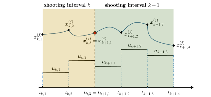
Figure 2: Sketch of the multi-shooting setting for the optimal control of one-dimensional deterministic problem. Shown are the piece-wise constant approximation of the control $\bm{u}(t)$, and the piece-wise differentiable approximation of the state $\bm{x}(t)$.

To ensure the continuity of each path across different shooting intervals, one can impose the continuity constraints

$$\bm{x}^{(i)}_{k+1,1}=\bm{x}^{(i)}_{k,N_{k}},\qquad i=1,\ldots,M.$$ (7)

However, this formulation introduces a very large number of optimization constraints (one for each sample path), making the discrete optimization problem very hard to solve. In fact, a large number constraints usually increases the computational cost, and the size of unfeasible regions. Therefore, instead of adding one continuity constraint for each sample path, we introduce a single constraint for each dimension and each partition, but across all sample paths.

$$\frac{1}{M}\sum_{l=1}^{M}\left(\bm{x}^{(l)}_{k,N_{k}}-\bm{x}^{(l)}_{k+1,1}\right)^{2}=0$$ (8)

which still guarantees continuity of sample trajectories across different shooting intervals, but in a way that is agnostic about the trajectory labels. In other words, across different shooting intervals the constraint (8) allows for a reshuffling of the trajectories labels. As is well know, this does not affect the computation of ensemble statistical properties (see Figure 3).

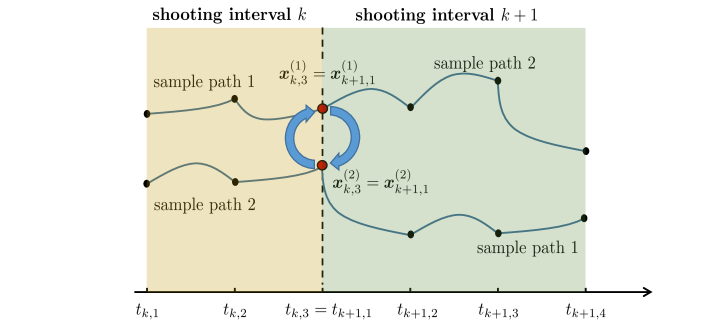
Figure 3: Continuity of sample paths across shooting intervals. The continuity constraint (8) allows us to re-label sample paths at the boundary of each shooting segment. This does not affect ensemble statistical properties at all, but it massively reduces the number of path continuity constraints (equality constraints in the optimizer) from $N$ to essentially one.

Approximating the integral in (6), e.g., with an explicit $s$-stage Adams-Bashforth [9] method yields

$$\bm{x}^{(i)}_{k,j+1}=\bm{x}^{(i)}_{k,j}+\Delta t_{k}\sum_{q=0}^{s-1}b_{j}\bm{f}\left(\bm{x}^{(i)}_{k,j-s},\bm{u}_{k,j-s}\right).$$ (9)

At this point it is convenient to denote the $i$th sample of the fully discrete state process in $[0,t_{f}]$ as

$$\bm{X}^{(i)}=\left\{\bm{x}^{(i)}_{1,1},\ldots\bm{x}^{(i)}_{1,N_{1}},\bm{x}^{(i)}_{2,1},\ldots,\bm{x}^{(i)}_{2,N_{2}},\ldots,\bm{x}^{(i)}_{S,1},\ldots,\bm{x}^{(i)}_{S,N_{S}}\right\},\qquad i=1,...,M.$$

It is also convenient to define a vector collecting the sample values the process $\bm{x}(t)$ at the boundaries of the shooting intervals, i.e.,

$$\bm{X}_{b}^{(i)}=\left\{\bm{x}^{(i)}_{1,1},\bm{x}^{(i)}_{1,N_{1}},\bm{x}^{(i)}_{2,1},\bm{x}^{(i)}_{2,N_{2}},\ldots,\bm{x}^{(i)}_{S,1},\bm{x}^{(i)}_{S,N_{S}}\right\},$$

and the full vectors of states and boundary values

$$\bm{X}=\left\{\bm{X}^{(1)},\ldots,\bm{X}^{(M)}\right\},\qquad\bm{X}_{b}=\left\{\bm{X}_{b}^{(1)},\ldots,\bm{X}_{b}^{(M)}\right\}.$$

Similarly, we denote the discrete control vector as

$$\bm{U}=\left\{\bm{u}_{1,1},\ldots\bm{u}_{1,N_{1}-1},\bm{u}_{2,1},\ldots,\bm{u}_{2,N_{2}-1},\ldots,\bm{u}_{S,1},\ldots,\bm{u}_{S,N_{S}-1}\right\}.$$

With this notation, we can write the fully discrete form of the optimal control problem (2) as

$$\begin{cases}\displaystyle\min_{\bm{U},\bm{X}_{b}}J(\bm{U},\bm{X}_{b})\\ \quad\text{subject to:}\\ \displaystyle\qquad\qquad\bm{x}^{(i)}_{k,j+1}=\bm{x}^{(i)}_{k,j}+\Delta t_{k}\sum_{q=0}^{s-1}b_{j}\bm{f}\left(\bm{x}^{(i)}_{k,j-s},\bm{u}_{k,j-s}\right),\quad\text{$\bm{x}_{1,1}^{(i)}$ random}\qquad\\ \displaystyle\qquad\qquad\sum_{k=1}^{S}\sum_{i=1}^{M}\left\|\bm{x}^{(i)}_{k,N_{k}}-\bm{x}^{(i)}_{k+1,1}\right\|_{2}^{2}=0\qquad\text{(path continuity constraint)}\vspace{0.2cm}\\ \displaystyle\qquad\qquad\bm{g}(\bm{U})\leq\bm{0}\qquad\textrm{(constraints on the control)}\\ \displaystyle\qquad\qquad\bm{h}(\mathbb{E}\{\bm{X}\})\leq\bm{0}\qquad\textrm{(ensemble path constraints)}\end{cases}$$ (10)

Remark 2.1

The first constraints in (10) is the discrete form of the ODE (1), i.e., it defines the temporal dynamics of each sample path under the control $\bm{U}$. In practice, all paths are pushed forward in time simultaneously for a given control by vectorizing the state vector in a way that includes all solution samples. Marching forward in time can take advantage of the massively parallel structure of the discretized ODE system.

3 Fast gradient computations

The large-scale constrained optimization problem (10) can be solved by using optimization algorithms based on gradient information. To this end, it is very important to be able to compute the gradient of the discretized cost function $J(\bm{U},\bm{X}_{b})$ with respect to the decision variables $(\bm{U},\bm{X}_{b})$, with accuracy and efficiency. In this section we provide technical details on how we implemented such gradient computation using automatic differentiation functions available in graph-based methods such as TensorFlow [1], and backward propagation. Our algorithm leverages the fact that forward time integration can be framed as a recurrent neural network, hence providing exact gradients at a negligible computational cost. Indeed, as we will see, all operations can be performed very efficiently on computational graphs.

3.1 Data-flow graphs

Modern machine learning techniques use decentralized data graphs to map computations in different nodes of a computer cluster [1]. Edges and nodes of such graph usually represent flows of data and input-output maps (operations), respectively. The dataflow graph is pre-compiled, optimized and stored as metadata in memory for the duration of the calculation. Using reverse automatic differentiation (backpropagation), the computational graph of the gradients with respect to a given cost function is simultaneously constructed and similarly stored. Using these two graphs one can integrate the system in time for a given control and compute gradients of the state trajectories with respect to the controls. The calculations are performed using a data event driven mechanism allowing for nearly simultaneous calculations of gradients as the dynamical system is being integrated. To illustrate the main idea, consider the follow dynamical system modeling the wheel-driving Unmanned Ground Vehicle (UGV) shown in Fig.4(a).

$$\begin{dcases*}\dot{x}_{1}=Ru_{1}(t)\cos(x_{3})\\ \dot{x}_{2}=Ru_{1}(t)\sin(x_{3})\\ \dot{x}_{3}=Ru_{2}\end{dcases*}$$ (11)

Here, $(x_{1}(t),x_{2}(t))$ denotes the position of the vehicle on the Cartesian plane while $x_{3}(t)$ is the heading angle. The controls are $u_{1}(t)$ (velocity) and $u_{2}(t)$ (steering angle). For illustration purposes, we discretize (11) with the Euler forward scheme (one-step Adams Bashforth (9)). This yields,

$$\begin{dcases*}x_{1}(t_{k+1})=x_{1}(t_{k})+\Delta tRu_{1}(t_{k})\cos(x_{3}(t_{k}))\\ x_{2}(t_{k+1})=x_{2}(t_{k})+\Delta tRu_{1}(t_{k})\sin(x_{3}(t_{k}))\\ x_{3}(t_{k+1})=x_{3}(t_{k})+\Delta tRu_{2}(t_{k})\end{dcases*}.$$ (12)

This system of equations defines explicitly an input-output map of the form

$$\bm{x}_{k+1}=\bm{Q}(\bm{x}_{k},\bm{u}_{k}).$$ (13)

Such map takes in $\bm{x}_{k}=[x_{1}(t_{k}),x_{2}(t_{k}),x_{3}(t_{k})]$ and $\bm{u}_{k}=[u_{1}(t_{k}),u_{2}(t_{k})]$ (which we assumed constant within the time interval $\Delta t$), and sends them to $\bm{x}(t_{k+1})$. Such nonlinear map can be conveniently represented as a “black box” with inputs $\bm{x}(t_{k})$ and $\bm{u}(t_{k})$, and output $\bm{x}(t_{k+1})$ as illustrated in Figure 5. It is clear at this point that the process of integrating the state vector $\bm{x}(t_{0})$ forward in time from $t_{0}$ to $t_{N}=t_{f}$ for any given piece-wise constant (in time) control

$$\bm{U}=\left[\bm{u}(t_{0}),\cdots\bm{u}(t_{N-1})\right]$$

can be seen as a composition of the same nonlinear map (12). This essentially defines a recurrent network that allows for an extremely low memory footprint and fast gradient computation.

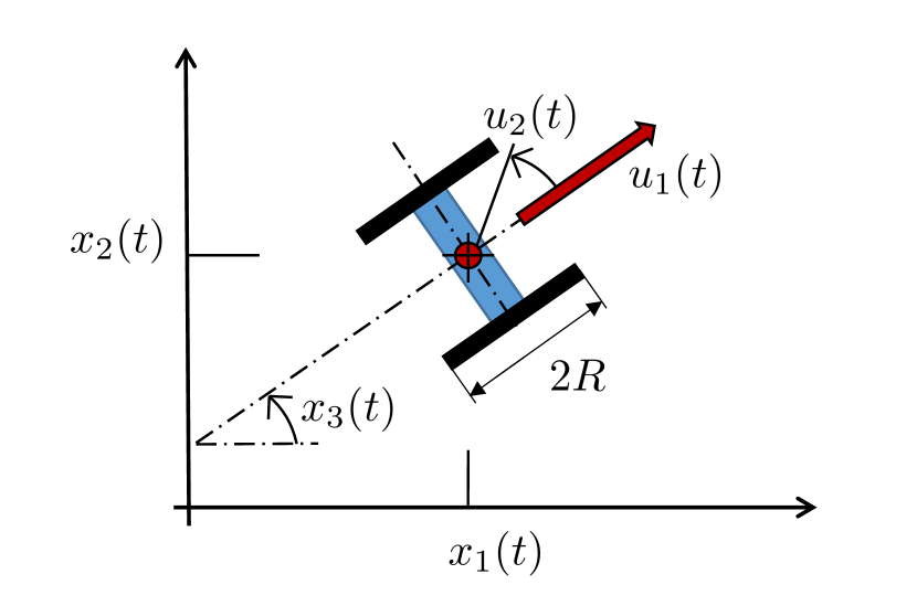
(a) UGV modeled by the system (11).

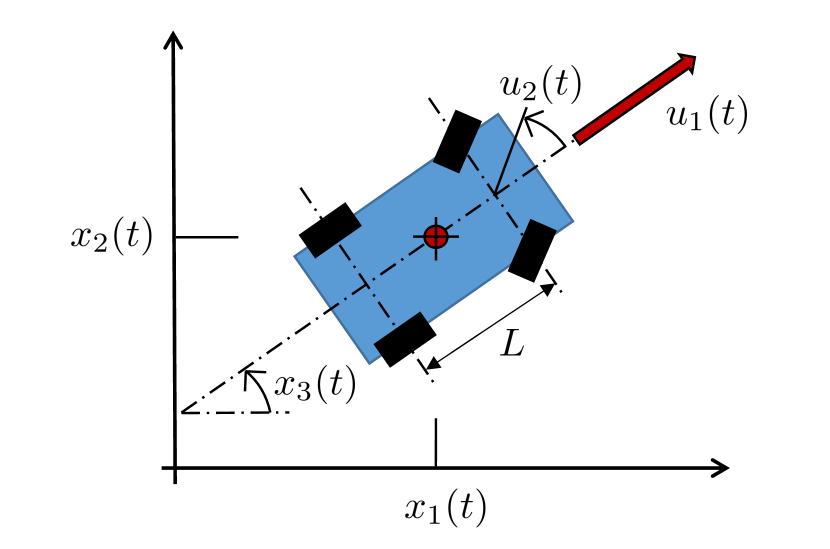
(b) UGV modeled by the system (16).

Figure 4: Sketches of two different Unmanned Ground Vehicles (UGVs). Shown are the state space variables $\{x_{i}(t)\}_{i=1,2,3}$, and the controls $u_{1}(t)$ and $u_{2}(t)$.

Moreover, as clearly seen from the computational graph sketched in Figure 5, portions of the calculations for the forward trajectory propagation as well as the backward gradient calculation are shared. Using reactive programming such shared portions of the graphs are computed only once, while memoization realizes additional substantial computational savings. The exact amount of savings depends on the efficiency of the graph compiler as well as the particular dynamics. Once the compiler creates and compiles the data graph in memory for a single trajectory, adding a dimension for sampling does not involve any changes to the graph or gradient calculations. By choosing a non-adaptive integration scheme, we ensure that the operations can be performed in lock step mode across all samples, and can utilize hardware with wide SIMD capabilities such as GPU, TPU or ASIC cards.

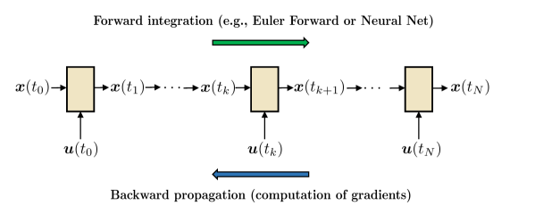
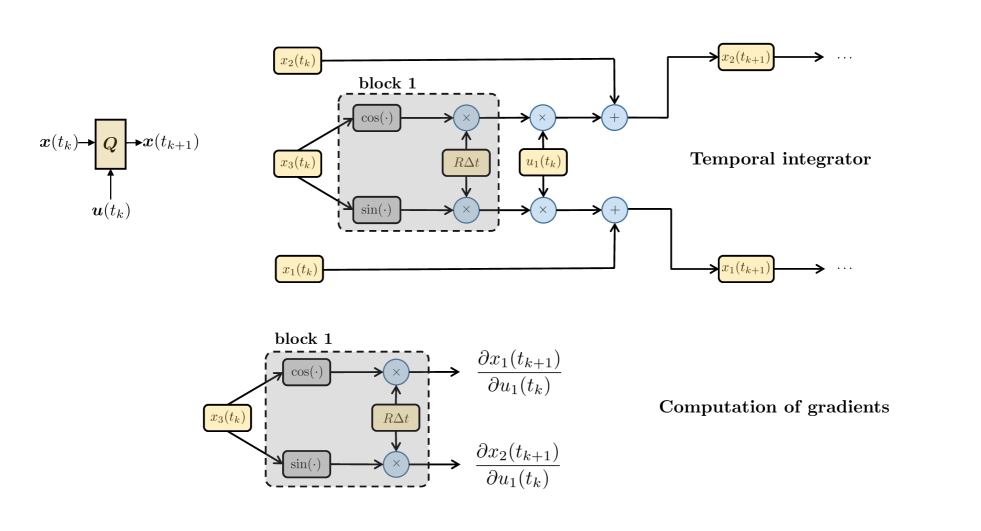
Figure 5: Portion of the data graph for the UGV model discretized with Euler forward time integration and graph the compute the kth component of the gradient of the cost functional. Note that there are sub-graphs that are shared among the computations (boxed graphs). Using reactive programming, all operations within such boxes are computed only once, and then shared across the graph.

3.2 Memory reduction and accelerated computations via Common Sub-expression Elimination (CSE)

Graph based methods for gradient calculations utilized by Deep Neural Net frameworks are scalable and are implemented in a computationally efficient way. However because they are designed to operate on large system for prolonged periods of time, ranging from hours to months, they have the following disadvantages:

1. They consume an inordinate amount of memory of the order of tens of gigabytes, especially for systems that have many constraints.

2. They use lazy initialization which makes the initial ramp up time very slow, often lasting hours for high dimensional systems with long time horizons. This is acceptable for deep neural net architectures, but hampers the response time for solving high dimensional optimal control problem.

3. Because of the hefty memory and time initialization requirements, they are unsuitable for online (real-time) applications, in particular those targeting autonomous vehicles.

The main idea around common sub-expression elimination is the observation that during the construction of the computational graph in systems like Tensorflow, the memory increases linearly with the number of steps. However since the computations are identical from on time step to the next, this motivates the objective of eliminating the common repeated calculations for each trajectory in order to save memory while not sacrificing computational speed, hence the name common sub-expression elimination.

To illustrate the basic idea of CSE in a simple way, let us consider (1) and write the time-discrete form as a symbolic nonlinear one-step recursion of the form (13). Suppose we are interested in minimizing a cost function of the form

$$J(\bm{U})=\frac{1}{M}\sum_{i=1}^{M}F(\bm{x}^{(i)}(t_{f})),$$ (14)

where $F$ is smooth. The gradient of (14) with respect to $\bm{u}(t_{k})$ can be computed using the chain rule as

$$\frac{\partial J(\bm{U})}{\partial\bm{u}(t_{k})}=\frac{1}{M}\sum_{i=1}^{M}\frac{\partial F(\bm{x}^{(i)}_{N})}{\partial\bm{x}}\frac{\partial\bm{Q}(\bm{x}^{(i)}_{N-1},\bm{u}_{N-1})}{\partial\bm{x}}\cdots\frac{\partial\bm{Q}(\bm{x}^{(i)}_{k+1},\bm{u}_{k+1})}{\partial\bm{x}}\frac{\partial\bm{Q}(\bm{x}^{(i)}_{k},\bm{u}_{k})}{\partial\bm{u}}.$$ (15)

This is the well-know backward propagation formula in recurrent neural networks. Indeed, the gradient of $J$ is obtained by iteratively applying the Jacobian maps $\partial\bm{x}(t_{j})/\partial\bm{x}(t_{j-1})$ from $j=N$ to $j=k+1$. Contrary to commonly used patterns in graph methods, here we need to store in memory only one gradient and two Jacobian functions, i.e.,

$$\frac{\partial F}{\partial\bm{x}},\qquad\frac{\partial\bm{Q}(\bm{x},\bm{u})}{\partial\bm{x}},\qquad\text{and}\qquad\frac{\partial\bm{Q}(\bm{x},\bm{u})}{\partial\bm{u}},$$

where $\bm{Q}$ is defined in (13). Even though other memory efficient schemes exist where the Jacobians are not stored explicitly, but rather the Jacobian vector product is done explicitly at each forward step, our numerical experiments indicate that storing the Jacobian explicitly strikes the best balance between computational efficiency and memory consumption. Moreover, the Jacobians for dynamical systems are of much smaller size than the Jacobians for neural nets, especially when the number of hidden layers in the latter is large, which explains why Jacobians are not stored explicitly in neural net frameworks. Taking advantage of the linear nature of the contribution of each trajectory of the ensemble to the end objective, we can leverage this linearity to customize the memory utilization through the mechanism of batching the samples. Specifically, a hundred-dimensional dynamical system over one thousand time steps requires a mere 100MB of memory per sample which is insignificant by today’s standards. On a modest embedded system or a GPU with 10GB or more in memory, this allows for the simultaneous propagation of one hundred trajectories per batch using SIMD instructions. For smaller systems, much larger batches of samples can be propagated simultaneously. The specific number of optimal samples that can be propagated in a single batch needs to be determined by experimentation on the particular hardware architecture in question. The overall number of samples propagated can therefore be as large as required by the problem in question, without increase in memory footprint.

3.2.1 Common Sub-expression Elimination: An example

It is difficult to quantify theoretically the memory and speed of graph-based methods to compute gradients such as (15) . Hence, in this section we illustrate the memory savings and computational speedup we obtained through a series of numerical experiments. To this end, we consider the following model of wheel-driving UGV

$$\dot{x}_{1}=u_{1}\cos(x_{3}),\qquad\dot{x}_{2}=u_{1}\sin(x_{3}),\qquad\dot{x}_{3}=\frac{u_{1}}{L}\tan(u_{2}),$$ (16)

where $(x_{1}(t),x_{2}(t))$ is the position of the vehicle, $x_{3}(t)$ is the heading angle, $u_{1}(t)$ is the forward velocity, and $u_{2}(t)$ is the steering angle (controls) – see Figure 4(b). We set the following box constraints on the controls

$$-1\leq u_{1}(t)\leq 1,\qquad-1\leq u_{2}(t)\leq 1\qquad\forall t\in[0,t_{f}].$$

We integrate (16) in time from $t_{0}=0$ to $t_{f}=100$ using an explicit Runge Kutta 4th order method with step size $\Delta t=0.1$ (i.e., a total of $N=1000$ steps) and with a fixed, randomly generated, controls $u_{1}$ and $u_{2}$. Recall that in the multi-shooting setting we consider here, the controls are assumed to be constant over each given time interval $[t_{i},t_{i+1}]$ (see Figure 2). To compute the gradient (15), hereafter we consider four different approaches, i.e.,

1. Second-order centerd finite differences (FD)

2. Operator overloading algorithmic differentiation (ADOLC [27])

3. Graph-based algorithmic differentiation implemented in TensorFlow [1] (TF)

4. Common Sub-expression Elimination (CSE)

and compare them in terms of memory consumption, speed and accuracy. Owing to lack of an analytical solution, we will use ADOLC [27], a mature algorithmic differentiation package to provide the benchmark gradient. In this example we consider an objective that is the simple average of the UGV squared distance to the origin, namely

$$J(\bm{U})=\frac{1}{M}\sum_{i=1}^{M}\left[x_{1}^{(i)}(t_{f})\right]^{2}+\left[x_{2}^{(i)}(t_{f})\right]^{2},$$ (17)

where $M$ is the number of sample paths. In Figure 6 we compare the absolute error in computing the gradient $\partial J/\partial u(t_{j})$ for each $t_{j}$ in $[0,100]$. It is seen that CSE and tensor flow are numerically exact, while second order (centered) finite-differences have accuracy of order $10^{-7}$, corresponds to the threshold we set. Lower precision in gradient calculations typically results in more iterations during optimization when utilizing interior point methods.

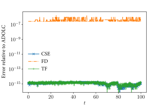
Figure 6: Absolute error of $\partial J/\partial u_{1}(t)$ with respect to the benchmark gradient computed with ADOLC for CSE, second-order centered finite differences (FD) and TensorFlow (TF). It is seen that tensor flow and CSE are numerically exact.

Next, we compare ADOLC, second-order finite-differences, tensorflow and CSE in terms of speed and memory consumption. This is done in Figure 7 and Figure 8, respectively. All numerical experiments were conducted on dual Xeon E5-2651 v2 processors operating at 1.80GHz with 145 GB of memory. For equivalence no GPUs were used. ADOLC appears to scale best for very large samples, but it is slower for samples below $M=10^{5}$ because of its lack of vectorization capabilities.

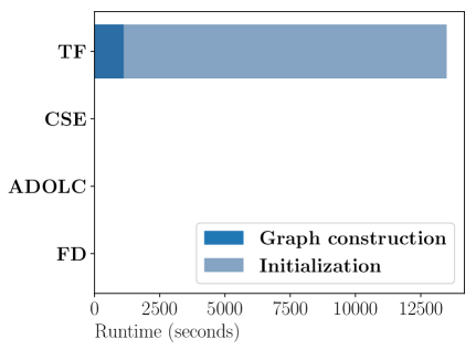
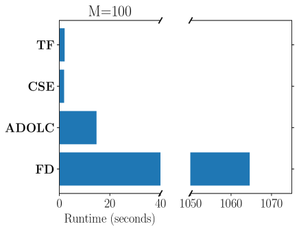
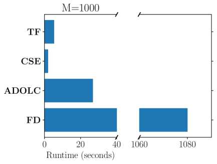
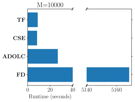
Figure 7: Execution times in seconds for different gradient methods. Here TF stands for tensorflow, and FD represents second-order finite differences. The CSE algorithm uses batch sizes of 100 samples for each thread, whereas ADOLC is parallelized one sample at a time. Tensorflow automatically optimizes its configuration for the target hardware architecture. Note the clear disadvantage in runtime that finite difference methods exhibit. All numerical experiments were conducted on a dual Xeon E5-2651 v2 processor workstation operating at 1.80GHz with 145 GB of memory.

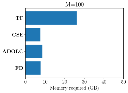
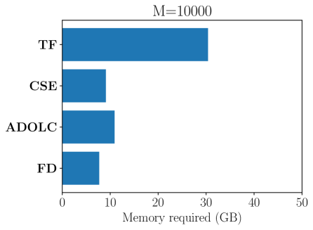
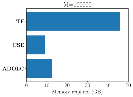
Figure 8: Memory consumption for different gradient calculation methods. Note that Tensorflow (TF) has the highest memory footprint, which grows substantially with sample size. On the other hand, CSE, ADOLC and fnite-differences (FD) have fairly constant memory footprints. All numerical experiments were conducted on a dual Xeon E5-2651 v2 processor workstation operating at 1.80GHz with 145 GB of memory.

The numerical experiments we presented in this section suggest that CSE and ADOLC and both suitable algorithms for ensemble gradient calculations. CSE is faster and more memory efficient and can be vectorized on GPU devices, wheres ADOLC is currently restricted to run on CPUs. Tensorflow is extremely fast and suitable for solving only smaller problems because of its memory consumption and very long initialization times.

4 Verification and validation of optimal controls

In this section we propose a new criterion to verify and validate the numerical solution to the optimal control problem (2). The criterion is based on the stochastic Pontryagin’s minimum principle [16, 12]. To describe method, consider the optimal control problem (2) and set

$$J([\bm{x}(t)],[\bm{u}(t)])=\mathbb{E}\left\{F(\bm{x}(t_{f}))\right\}+\int_{0}^{t_{f}}r(\bm{u}(\tau))d\tau,$$ (18)

$r$, and $F$ being given functions. The second term at the right hand side is usually referred to as “control energy” term, and it can provide regularization of the optimization problem. Let us define the Hamilton’s function

$$H(\bm{u},\bm{x},\bm{\lambda})=r(\bm{u})+\bm{\lambda}\cdot\bm{f}(\bm{x},\bm{u}).$$ (19)

From this we obtain the Hamilton’s equations

$$\begin{dcases*}\dot{\bm{x}}=\frac{\partial H}{\partial\bm{\lambda}}=\bm{f}(\bm{x},\bm{u}),\\ \dot{\bm{\lambda}}=-\frac{\partial H}{\partial\bm{x}}=-\frac{\partial\bm{f}}{\partial\bm{x}}\cdot\bm{\lambda}.\end{dcases*}$$ (20)

As shown in [16], the system (20) is supplemented with a (random) initial condition for $\bm{x}(t)$, and a final condition for $\bm{\lambda}(t)$

$$\bm{x}(0)=\bm{x}_{0}(\omega),\qquad\bm{\lambda}(t_{f})=\frac{\partial F(\bm{x}(t_{f}))}{\partial\bm{x}}.$$ (21)

In other words, (20)-(21) is a two-point boundary value problem. Given any control $\widehat{\bm{u}}(t)$, we can solve (20)-(21) using forward-backward propagation as illustrated in Figure 9. How can we check whether $\widehat{\bm{u}}(t)$ is optimal, i.e., it solves (2)-(18)? A necessary condition is that the control satisfies the following minimization principle (extended Pontryagin’s principle)

$$\bm{u}^{*}(t)=\operatorname*{\arg\!\min}_{\bm{u}(t)}\mathbb{E}\{H({\bm{u}}(t),\bm{x}(t),\bm{\lambda}(t)\}\qquad\forall t\in[0,t_{f}],$$ (22)

subject to the Hamilton’s equations (20)-(21), and the constraints $\bm{g}(\bm{u}(t))\leq\bm{0}$ on the control $\bm{u}(t)$. Note that both $\bm{x}(t)$ and $\bm{\lambda}(t)$ in (22) are functionals of $\bm{u}(t)$. The Pontryagin’s principle (22) offers us a simple way to verify the optimality of a given control. To this end, suppose we have available a solution of (2), say $\widehat{\bm{u}}(t)$, computed using an optimizer, and we want to verify whether such solution is indeed optimal. A possible way to perform this calculation is to sample a large number of initial states $\bm{x}_{0}(\omega)$ and propagate them through the forward/backward problem (20)-(21). This allows us to obtain many realizations of $\bm{x}^{(i)}(t)$ and $\bm{\lambda}^{(i)}(t)$ for the given candidate control $\widehat{\bm{u}}(t)$. With such realizations available, we can approximate the expectation in (22) using, e.g., Monte Carlo and compute

$$\bm{u}^{*}(t)=\operatorname*{\arg\!\min}_{\bm{u}(t)}\frac{1}{M}\sum_{i=1}^{M}H\left(\bm{u},\bm{x}^{(i)}(t),\bm{\lambda}^{(i)}(t)\right).$$ (23)

At this point we can compare $\bm{u}^{*}(t)$ with $\widehat{\bm{u}}(t)$ and verify whether the two controls are close to each other.

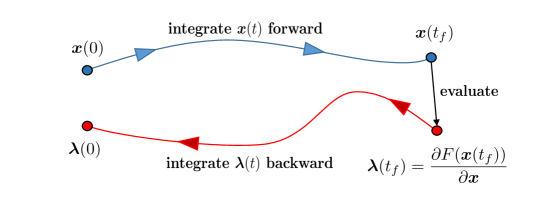
Figure 9: Schematic of the forward-backward integration process for validation and verification of optimal controls.

5 Numerical applications

In this section we demonstrate the proposed optimal control algorithms in applications to stochastic path planning problems involving models of an unmanned ground vehicles (UGVs) and a fixed-wing unmanned aerial vehicles (UAVs).

5.1 UGV stochastic path planning problem

Consider the systems of equations (11), describing the dynamics of a simple two-wheeled UGV with differential drive. We would like to control the velocity $u_{1}(t)$ and the steering angle $u_{2}(t)$ of the UGV in in a way that the vehicle hits a target located at $(x_{1},x_{2})=(3,3)$ at time $t_{f}=10$. To this end, we first assume that the initial state of the system is deterministic, i.e.,

$$x_{1}(0)=0,\qquad x_{2}(0)=0,\qquad x_{3}(0)=0,\qquad R=1.25.$$ (24)

Moreover, we assume that the controls $u_{1}(t)$ and $u_{2}(t)$ are subject to the following constraints

$$-1\leq u_{1}(t)\leq 1,\qquad-1\leq u_{2}(t)\leq 1.$$ (25)

We determined the optimal control for this deterministic problem by minimizing the objective functional

$$J([u_{1}(t),u_{2}(t)])=\frac{1}{2}\left\{\left(x_{1}(t_{f})-3\right)^{2}+\left(x_{2}(t_{f})-3\right)^{2}\right\}+\frac{q}{2}\int_{0}^{t_{f}}\left[u_{1}(t)^{2}+u_{2}(t)^{2}\right]dt.$$ (26)

with respect to $u_{1}(t)$ and $u_{2}(t)$. Note that $x_{1}(t_{f})$ and $x_{2}(t_{f})$ are both functionals of $(u_{1}(t),u_{2}(t))$. We will refer to the controls minimizing (26) subject to the dynamics (11), the initial condition (24) and the constraints (25) as the nominal controls. This nominal control is used as the initial guess for the stochastic version of the problem, which can be formulated as follows: find controls $\{u_{1}(t),u_{2}(t)\}$ maximizing the probability that the UGV hits a target located at $(x_{1},x_{2})=(3,3)$ at $t_{f}=10$ under uncertain initial conditions and wheel radius $R$. In particular, we model such uncertainty as uniformly distributed independent random variables

$$x_{1}(0)\sim\mathcal{U}(-0.05,0.05),\ \ x_{2}(0)\sim\mathcal{U}(-0.05,0.05),\ \ x_{3}(0)\sim\mathcal{U}(-0.05,0.05),\ \ R\sim\mathcal{U}(1,1.5).$$ (27)

Note that the wheel radius $R$ here is assumed to be random. The stochastic version of the functional (26) can be written as

$$J([u_{1}(t),u_{2}(t)])=\frac{1}{2}\mathbb{E}\left\{\left(x_{1}(t_{f})-3\right)^{2}+\left(x_{2}(t_{f})-3\right)^{2}\right\}+\frac{q}{2}\int_{0}^{t_{f}}\left[u_{1}(t)^{2}+u_{2}(t)^{2}\right]dt,$$ (28)

where $\mathbb{E}\{\cdot\}$ denotes an expectation over the (jointly uniform) PDF of $x_{1}(0)$, $x_{2}(0)$, $x_{3}(0)$, and $R$. The optimal control problem reads as follows: minimize (28) subject the dynamics (25), initial codnitions (27) and control constraints (25). The integral in both (26) and (28) represents the energy of the control, and it provides a regularization of the control profiles, even for very small values of $q$. To compute the nominal and the optimal controls we utilized the multi-shooting algorithm we described in Section 2, with $S=2$ shooting intervals, explicit RK4 time integration ($\Delta t=0.05$), and CSE (section 3.2) to calculate the ensemble gradient of the cost functional (see Eq. (15)). The number of sample paths to approximate the expectation in (28) with a Monte Carlo cubature were set to $M=10000$. This yields a fully discrete optimal control problem of the form (10) (with no path constraints), which we solved using IPOPT [26, 3, 32] linked with CSE and verified using Tensorflow (see Section 3). The results of our simulations are summarized in Figure (10). We see that, as expected, the final position of the UGV under nominal and optimal controls is clustered around the target located at $(x_{1},x_{2})=(3,3)$. However, in the optimal control case, to reduce the variance of the set of trajectories at final time, the UGV does not head directly towards the target, but it initially heads rights and then takes a steep left turn. On the other hand, in the nominal control case, the UGV heads directly towards the target, but the set of trajectories at final time is more spread out around the target than in the optimal control case.

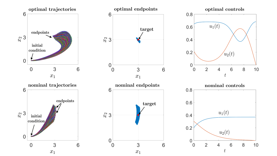
Figure 10: UGV stochastic path planning problem. Stochastic dynamics under optimal and nominal controls. It is seen that in both cases the endpoints of the UGV trajectories are clustered around the target located at $(x_{1},x_{2})=(3,3)$. However, in the optimal control case, to reduce the variance of the set of trajectories at final time, the UGV does not head directly towards the target, but it initially heads rights and then takes a steep left turn. On the other hand, in the nominal control case, the UGV heads directly towards the target, but the set of trajectories at final time is more spread out around the target than in the optimal control case.

For verification and validation of the optimal controls, we analytically derive the Hamiltonian function for the system (11)

$$H(\bm{u},\bm{x},\bm{\lambda})=\frac{q}{2}\left(u_{1}^{2}+u_{2}^{2}\right)+\lambda_{1}Ru_{1}\cos(x_{3})+\lambda_{2}Ru_{1}\sin(x_{3})+\lambda_{3}Ru_{2}.$$ (29)

The adjoint system is given by

$$\begin{dcases*}\dot{\lambda}_{1}=0,\\ \dot{\lambda}_{2}=0,\\ \dot{\lambda}_{3}=\lambda_{1}Ru_{1}(t)\sin(x_{3})-\lambda_{2}Ru_{1}(t)\cos(x_{3}).\end{dcases*}$$ (30)

We follow the process described in section 4 to measure the optimality of the computed solution. This is done in Figure 11, where we compare the control $\bm{u}^{*}(t)=\{u_{1}^{*}(t),u_{2}^{*}(t)\}$ we obtained by solving (23) with optimal control $\widehat{\bm{u}}$ that minimizes (28). It is seen that the two controls are very close to each other, which means that $\widehat{\bm{u}}$ is a good approximation to the optimal control.

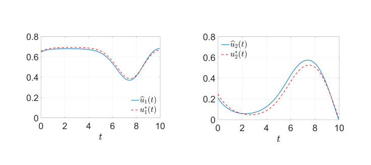
Figure 11: UGV stochastic path planning problem. Verification and Validation of the optimal control using the extended Pontryagin’s minimum principle presented in Section 4.

5.2 UAV stochastic path planning problem

In this section we consider a more challenging problem, namely stochastic path planning for a fixed-wing unmanned aerial vehicle (UAV) model under uncertain initial state such as position, heading angle, angle of attach and aerodynamic forces. The nonlinear dynamical system modeling the UAV is [18, 19]:

$$\begin{cases*}\dot{x}=v\cos\gamma\cos\sigma\\ \dot{y}=v\cos\gamma\sin\sigma\\ \dot{z}=v\sin\gamma\\ \dot{v}=\displaystyle\frac{1}{m}(-D+T\cos\alpha)-g\sin\gamma\\ \dot{\gamma}=\displaystyle\frac{1}{mv}(L\cos\mu+T\cos\mu\sin\alpha)-\frac{g}{v}\cos\gamma\\ \dot{\sigma}=\displaystyle\frac{1}{mv\cos\gamma}(L\sin\mu+T\sin\mu\sin\alpha)\\ \dot{T}=u_{T}\\ \dot{\alpha}=u_{\alpha}\\ \dot{\mu}=u_{\mu}\end{cases*}$$ (31)

where $(x(t),y(t),z(t))$ is the position of the UAV in a Cartesian reference frame, $v(t)$ is the velocity, $(\gamma(t),\sigma(t))$ are elevation and heading angles, $T(t)$ is the thrust, $\alpha(t)$ is the angle of attack, and $\mu(t)$ is the bank angle (see Figure 12). The UAV model (31) is valid only in the region of the phase space defined by the following constraints

$$13\leq v(t)\leq 42,\quad-\frac{\pi}{6}\leq\gamma(t)\leq\frac{\pi}{6},\quad-\pi\leq\sigma(t)\leq\pi,\quad 3.0\leq T(t)\leq 35.0,\quad-\frac{\pi}{8}\leq\alpha(t)\leq\frac{\pi}{8}.$$ (32)

These are effectively linear state space constraints that needs to be added to the optimal control problem (see Eqs. (2) and (10)).

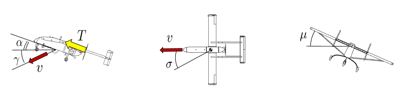
Figure 12: Sketch of the fixed wing Unmanned Aerial Vehicle (UAV). Shown are some of the phase variables appearing in the model (31). The controls act on the trust $T$, the angle of attack $\alpha$, and the bank angle $\mu$.

The other parameters appearing in (31) are the UAV mass $m=2$ kg, the acceleration of gravity $g=9.8$ m/s², and the aerodynamic lift and drag forces given by

$$L=\frac{1}{2}\rho v^{2}SC_{L},\qquad D=\frac{1}{2}\rho v^{2}SC_{D},$$ (33)

In these expressions $\rho(z)=1.21e^{-z/8000}$ kg/m³ is the mass density of air, $S=0.982$ m² is the wing surface area, and $C_{L}$ and $C_{D}$ are the lift and drag coefficients defined as

$$C_{L} =(C_{x0}+C_{xa}\alpha)\sin\alpha-(C_{z0}+C_{za}\alpha)\cos\alpha,$$ (34)

$$C_{D} =-(C_{x0}+C_{xa}\alpha)\cos\alpha-(C_{z0}+C_{za}\alpha)\sin\alpha.$$ (35)

Note that $C_{L}$ and $C_{D}$ depend on the parameters $C_{x0},C_{xa},C_{z0},$ and $C_{za}$ which are usually unknown and must be estimated from data. In our simulation we model such coefficients as independent random variables with given probability distributions.

We aim at computing optimal controls for the angle of attach $u_{\alpha}(t)$, the bank angle $u_{\mu}(t)$ and trust $u_{T}(t)$ so that the UAV hits the target located at $(x,y,z)=(500,500,500)$ under uncertain aerodynamic forces, uncertain initial position/angles, and uncertain initial velocity. The controls are subject to the following box constraints.

$$u_{T}\in[-1.0,1.0],\qquad u_{\alpha}\in[-0.05,0.05],\qquad u_{\mu}\in[-0.05,0.05].$$ (36)

Following the same steps as in the UGV example we studied in section 5.1, we first calculate the nominal control where we minimize the functional

$$J\left([u_{T}(t)],[u_{\alpha}(t)],u_{\mu}(t)]\right)= (x(t_{f})-500)^{2}+(y(t_{f})-500)^{2}+(z(t_{f})-500)^{2}+$$

$$\frac{1}{200}\int_{0}^{t_{f}}\left[u_{T}^{2}(t)+u_{\alpha}^{2}(t)+u_{\mu}^{2}(t)\right]dt$$ (37)

subject to (31), (32), (36) and the deterministic initial states

$$x(0)=0,\quad y(0)=0,\quad z(0)=0,\quad v(0)=27.5,\quad\gamma(0)=0,\quad\sigma(0)=\pi,\quad T(0)=16.1,$$

$$\alpha(0)=-0.0088,\quad\mu(0)=0,\quad C_{x0}=-0.03554,\quad C_{xa}=0.00292,\quad C_{z0}=-0.055,\quad C_{za}=-5.578.$$

Note that this defines a challenging maneuver whereby the UAV has to move from $(x(0),y(0),z(0))=(0,0,0)$ to $(x(t_{f}),y(t_{f}),z(t_{f}))=(500,500,500)$ while the initial heading angle $\sigma$ is in the opposite direction (see Figure 14(a)).

Next, we consider the stochastic path planning problem, i.e., the problem of computing robust controls that can steer the UAV from an uncertain initial state (position, velocity, and configuration angles) to the final position $(x(t_{f}),y(t_{f}),z(t_{f}))=(500,500,500)$, under random aerodynamics forces. A simplified version of this problem was recently studied by Shaffer et. al in [19], where uncertainty was modeled in terms of only one random variable, i.e., $C_{x0}$ in Eqs. (34) and (35). The main reason for studying such simplified model was that the computational control algorithm could not handle higher-dimensional random input vectors. Indeed, the memory requirements and computational cost of the algorithms proposed in [19] are currently beyond the capabilities of a modern workstation. To compute the optimal controls in the stochastic path planning UAV problem we minimize the cost functional

$$J\left([u_{T}(t)],[u_{\alpha}(t)],[u_{\mu}(t)]\right)= \mathbb{E}\left\{(x(t_{f})-500)^{2}+(y(t_{f})-500)^{2}+(z(t_{f})-500)^{2}\}\right\}+$$

$$\frac{1}{200}\int_{0}^{t_{f}}\left[u_{T}^{2}(t)+u_{\alpha}^{2}(t)+u_{\mu}^{2}(t)\right]dt,$$ (38)

subject to (31), (32), the random initial condition

$$x(0)=r\sin(\theta)\cos(\phi),\qquad y(0)=r\sin(\theta)\sin(\phi),\qquad z(0)=r\cos(\phi),$$ (39)

$$v(0)\sim\mathcal{U}(25.5750,29.4250),\qquad\gamma(0)\sim\mathcal{U}(-0.05,0.05),\qquad\sigma(0)\sim\mathcal{U}(3.1,3.2),$$ (40)

$$C_{x0}\sim\mathcal{U}(-0.0380,-0.0330),\qquad C_{xa}\sim\mathcal{U}(0.0027,0.0031),$$

$$C_{z0}\sim\mathcal{U}(-0.0589,-0.0548),\qquad C_{za}\sim\mathcal{U}(-5.9685,-5.1875),$$ (41)

where $r\sim\mathcal{U}(0,5.0)$, $\theta\sim\mathcal{U}(0,\pi)$ $\phi\sim\mathcal{U}(0,2\pi)$, and the ensemble path constraints

$$13\leq\mathop{\mathbb{E}}\{v(t)\}\leq 42,\qquad-\frac{\pi}{6}\leq\mathop{\mathbb{E}}\{\gamma(t)\}\leq\frac{\pi}{6},\qquad-\pi\leq\mathop{\mathbb{E}}\{\sigma(t)\}\leq\pi,$$

$$3.0\leq\mathop{\mathbb{E}}\{T(t)\}\leq 35.0,\qquad-\frac{\pi}{12}\leq\mathop{\mathbb{E}}\{\alpha(t)\}\leq\frac{\pi}{12}.$$

In Eqs. (5.2) and (31) $\mathbb{E}\{\cdot\}$ is an expectation over the joint PDF of the random variables in the initial state, which we approximate using Monte Carlo cubature rule with $M=4800$ randomly drawn sample paths.

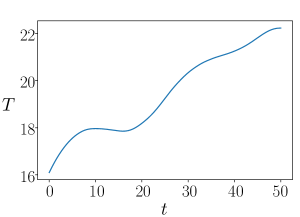
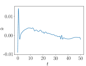
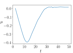
Figure 13: Stochastic path planning problem for the fixed-wing UAV model (31). Shown are the optimal trust $T(t)$, angle of attack $\alpha(t)$ and bank angle $\mu(t)$ (integrals of $u_{T}$, $u_{\alpha}$ and $u_{\mu}$) we obtained to steer the UAV from the random initial position (39) to the final position $(x,y,z)=(500,500,500)$, under random aerodynamic forces.

To compute the nominal and the optimal controls we utilized a single shooting algorithm with explicit RK3 time integration ($\Delta t=0.1$), and CSE to calculate the ensemble gradient of the cost functional (see Eq. (15)). This yields a fully discrete optimal control problem of the form (10), which we solved using IPOPT [26, 3, 32] linked with CSE, and verified using ADOLC [27]. The optimal trust, angle of attack and bank angle are shown in Figure 13. To verify the performance of the optimal controls under random initial conditions and uncertain parameters, we propagated in time the controlled dynamics of $10000$ randomly generated trajectories, with initial conditions and parameters sampled according to (39)-(41). Such trajectories are shown in Figure 14. It is seen that the final positions of the UAV converge to a smaller region about the target location $(x,y,z)=(500,500,500)$.

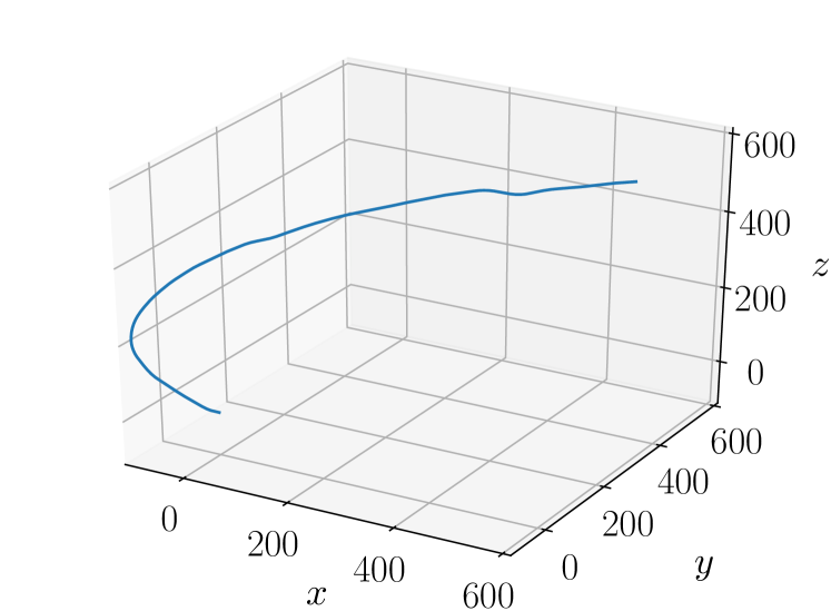
(a) Nominal trajectory.

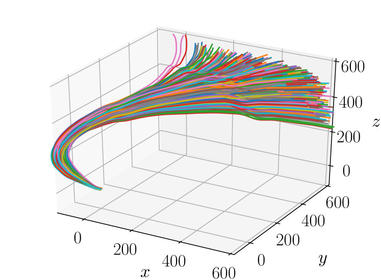
(b) Random trajectories under nominal controls.

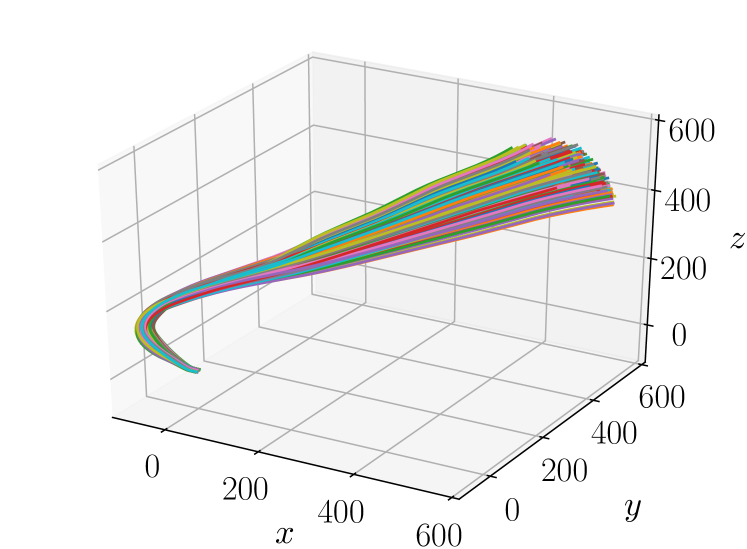
(c) Random trajectories under optimal controls.

Figure 14: UAV stochastic path planning problem. Shown are trajectories obtained by sampling the random initial condition and the random parameters of the model (31) and then propagating them forward in time using nominal and optimal controls. It is seen that the optimal controls can mitigate the effects of uncertainty, and they yield final states clustered around the target located at $(x,y,z)=(500,500,500)$. Figures drawn to the same scale for comparison.

5.2.1 Nonlinear advection-reaction-diffusion PDE

In this section we study open-loop control under uncertainty of nonlinear PDEs. Specifically, we consider the following initial-boundary value problem involving a nonlinear advection-reaction-diffusion equation

$$\left\{\begin{array}[]{ll}\displaystyle\frac{\partial\psi}{\partial t}=\psi\frac{\partial\psi}{\partial x}+\frac{1}{5}\frac{\partial^{2}\psi}{\partial x^{2}}+\frac{3}{2}\psi e^{-\psi/10}+I_{\Omega}(x)u(t),\vspace{0.2cm}\\ \psi(t,-1)=\psi(t,1)=0,\vspace{0.2cm}\\ \psi(0,x)=\psi_{0}(x),\end{array}\right.$$ (42)

where $\psi(x,t):[-1,1]\times[0,t_{f}]\mapsto\mathbb{R}$ is a random field that is a functional of $\psi_{0}$ (random initial condition) and $u(t):[0,t_{f}]\to\mathbb{R}$ (control). Note that $u(t)$ is actuated only on the spatial domain $\Omega=[-0.5,-0.2]$, which is the support of the indicator function $I_{\Omega}(x)$. We aim at determining the optimal control $u(t)$ that minimizes the cost functional

$$J([\psi],[u])=\frac{1}{2}\mathbb{E}\left\{\int_{-1}^{1}\psi(t_{f},x)^{2}dx+2\int_{0}^{t_{f}}\int_{-1}^{1}\psi(\tau,x)^{2}dxd\tau\right\}+\frac{1}{20}\int_{0}^{t_{f}}u(\tau)^{2}d\tau,\qquad t_{f}=8,$$ (43)

where $\mathbb{E}\{\cdot\}$ is an expectation over the probability distribution of the initial state $\psi_{0}(x)$. To this end, we first discretize (42) in space using a Chebyshev pseudo-spectral method [20]. This yields the semi-discrete form

$$\left\{\begin{array}[]{ll}\displaystyle\dot{\bm{\psi}}=\bm{\psi}\circ\bm{D}\bm{\psi}+\frac{1}{5}{\bm{D}}^{2}\bm{\psi}+\frac{3}{2}\bm{\psi}\circ e^{-\bm{\psi}/10}+\bm{I}_{\Omega}u(t),\vspace{0.2cm}\\ \bm{\psi}(0)=\bm{\psi}_{0},\end{array}\right.$$ (44)

where $\bm{\psi}(t)=[\psi(t,x_{1}),...,\psi(t,x_{n})]^{T}$ collects the values of the solution $\psi(t,x)$ at the (inner) Chebyshev nodes

$$x_{j}=\cos\left(\frac{j\pi}{n+1}\right)\qquad j=1,...,n.$$ (45)

In equation (44), the circle “$\circ$” denotes element-wise multiplication (Hadamard product), $\bm{I}_{\Omega}$ is the discrete indicator function, while $\bm{D}$ and $\bm{D}^{2}\in\mathbb{R}^{n\times n}$ are, respectively, the first- and second-order Chebyshev differentiation matrices. These matrices obtained by deleting the first and last rows and columns of the full differentiation matrices. In Figure 15 we plot two solution samples of the initial-boundary value problem (42) we obtained by integrating the discretized system (44) in time.

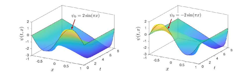
Figure 15: Solution samples of the initial-boundary value problem (42) corresponding to different initial conditions. Here we set the control $u(t)$ equal to zero (uncontrolled dynamics).

The cost functional (43) can be discretized as

$$J=\frac{1}{2M}\sum_{i=1}^{M}\bm{w}^{T}\left[\bm{\psi}^{(i)}(t_{f})^{2}+2\int_{0}^{t_{f}}\bm{\psi}^{(i)}(\tau)^{2}d\tau\right]+\frac{1}{20}\int_{0}^{t_{f}}u(\tau)^{2}d\tau,$$ (46)

where $\bm{w}$ are Clenshaw-Curtis quadrature weights (column vector), and $M$ is the total number of samples.

To quantify the effectiveness of the ensemble optimal control algorithm we propose, we first determine the nominal control corresponding to the deterministic initial condition $\psi_{0}(x)=2\sin(\pi x)$. Such control minimizes the functional (46) with $M=1$ and $\psi^{(1)}_{j}(0)=2\sin(\pi x_{j})$, and sends $\psi(t,x)$ to zero after a small transient (see Figure 16).

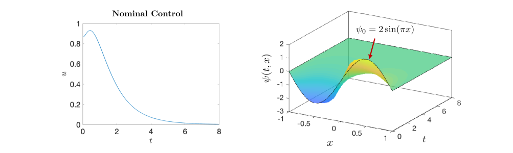
Figure 16: Open loop control of the nonlinear PDE (42). Shown is the nominal control minimizing (43) for the deterministic initial condition $\psi_{0}=2\sin(\pi x)$ and the corresponding solution dynamics. It is seen that the control $u(t)$ sends $\psi(t,x)$ to zero after a small transient.

Next, we introduce uncertainty in the initial condition. Specifically, we set

$$\bm{\psi}_{0j}=2\sin(\pi x_{j})+\epsilon_{j}\qquad\epsilon_{j}\sim\mathcal{N}(0,001).$$ (47)

This makes the solution to (42) and (44) stochastic. As seen in Figure 17 the introduction of this small uncertainty, causes large perturbations to the system solution under nominal control especially at t=8. To compute the optimal control, we minimized the functional (46) subject to $M=1000$ replicas of the dynamical system (44). Specifically, we considered the single-shooting setting described in section 2 with $\Delta t=0.0005$, Euler time integrator, and CSE gradient algorithm. In Figure 17 we compare the mean and the standard deviation of the solution we obtain by using nominal and optimal controls. It is that the optimal control is more effective is driving the solution ensemble to zero. In fact, both the mean and standard deviation of the optimally controlled dynamics are closer to zero. Note also that the optimal control differs substantially from the nominal control.

Figure 17: Comparison between the mean and the standard deviation of the stochastic solution to the PDE (42) under optimal or nominal controls. The initial condition here is set to be random as (47). It is seen that the optimal control is more effective is driving the stochastic solution to zero. In fact, both the mean and standard deviation of the optimally controlled solution are closer to zero. Note also that the optimal control differs substantially from the nominal control.

6 Summary

In this paper we developed a new scalable algorithm for computational optimal control under uncertainty. The new algorithm combines multi-shooting discretization methods, interior point optimization, common sub-expression elimination, and exact gradients obtained via automatic differentiation and computational graphs. It also allows for point-wise control constraints and ensemble state-space constraints. The algorithm has an extremely low memory footprint, which allows us to process a large number of sample trajectories and controls random dynamical systems over long time horizons. We also developed a new criterion for verification and validation of optimal control based on the stochastic version of the Pontryagin’s minimum principle. We demonstrated the accuracy and computational efficiency of the new algorithm in applications to stochastic path planning problems involving models of unmanned aerial and ground vehicles, and in distributed control of a nonlinear advection-reation-diffusion PDE.

Acknowledgements This research was developed with funding from the Defense Advanced Research Projects Agency (DARPA) grant FA8650-18-1-7842.

References

- [1] M. Abadi, P. Barham, J. Chen, Z. Chen, A. Davis, et al., et al. Tensorflow: a system for large-scale machine learning. In OSDI, volume 16, pages 265–283, 2016.
- [2] A. G. Baydin, B. A. Pearlmutter, A. A. Radul, and J. M. Siskind. Automatic differentiation in machine learning: a survey. Journal of Marchine Learning Research, 18:1–43, 2018.
- [3] L. T. Biegler and V. M. Zavala. Large-scale nonlinear programming using ipopt: An integrating framework for enterprise-wide dynamic optimization. Computers & Chemical Engineering, 33(3):575–582, 2009.
- [4] J. Dick, F. Y Kuo, and I. H. Sloan. High-dimensional integration: The quasi-Monte Carlo way. Acta Numerica, 22:133–288, 2013.
- [5] F. Fahroo and I. M. Ross. Costate estimation by a Legendre pseudospectral method. AIAA Journal of Guidance, Control and Dynamics, 24(2):270–277, 2001.
- [6] J. Foraker, J. O. Royset, and I. Kaminer. Search-trajectory optimization: Part I, formulation and theory. Journal of Optimization Theory and Applications, 169(2):530–549, 2016.
- [7] Q. Gong, W. Kang, I. M. Ross, and F. Fahroo. A pseudospectral method for the optimal control of constrained feedback linearizable systems. IEEE Trans. On Automatic Control, 51(7):1115–1129, 2006.
- [8] Q. Gong, I. M. Ross, and F. Fahroo. Spectral and pseudospectral optimal control over arbitrary grids. Journal of Optimization Theory and Applications, 169(3):759–783, 2016.
- [9] E. Hairer, C. Lubich, and G. Wanner. Geometric numerical integration: structure-preserving algorithms for ordinary differential equations. Springer, second edition, 2006.
- [10] M. J. Keeling and K. T. D. Eames. Networks and epidemic models. J. R. Soc. Interface, 2(4):295–307, 2005.
- [11] J. S. Li, J. Ruths, T. Y. Yu, H. Arthanari, and G. Wagner. Optimal pulse design in quantum control: A unified computational method. Proceedings of the National Academy of Sciences, 108(5):1879–1884, 2011.
- [12] C. Phelps, Q. Gong, J. O. Royset, C. Walton, and I. Kaminer. Consistent approximation of a nonlinear optimal control problem with uncertain parameters. Automatica, 50(12):2987–2997, 2014.
- [13] C. Phelps, J. O. Royset, and Q. Gong. Optimal control of uncertain systems using sample average approximations. SIAM Journal on Control and Optimization, 54(1):1–29, 2016.
- [14] S. C. Reddy and L. N. Trefethen. Stability of the method of lines. Numer. Math., 62:235–267, 1992.
- [15] A. Rodgers and D. Venturi. Stability analysis of hierarchical tensor methods for time-dependent pdes. arXiv, 1908.09803:1–20, 2019.
- [16] I. M. Ross, R. J. Proulx, M. Karpenko, and Q. Gong. Riemann–Stieltjes optimal control problems for uncertain dynamic systems. AIAA Journal of Guidance, Control, and Dynamics, 38(7):1251–1263, 2015.
- [17] A. Ruszczyński and A. Shapiro. Optimization of risk measures. In G. Calafiore and F. Dabbene, editors, Probabilistic and randomized methods for design under uncertainty, pages 119–157. Springer, 2006.
- [18] M. Savage. Design and hardware-in-the-loop implementation of optimal canonical maneuvers for an autonomous planetary aerial vehicle. Master’s thesis, Naval Postgraduate School, Monterey, California, 2012.
- [19] R. Shaffer, M. Karpenko, and Q. Gong. Unscented guidance for waypoint navigation of a fixed-wing UAV. In 2016 American Control Conference (ACC), pages 473–478, July 2016.
- [20] L. N. Trefethen. Spectral Methods in MATLAB. Society for Industrial and Applied Mathematics, 2000.
- [21] D. Venturi. The numerical approximation of nonlinear functionals and functional differential equations. Physics Reports, 732:1–102, 2018.
- [22] D. Venturi, H. Cho, and G. E. Karniadakis. The Mori-Zwanzig approach to uncertainty quantification. In R. Ghanem, D. Higdon, and H. Owhadi, editors, Handbook of uncertainty quantification. Springer, 2016.
- [23] D. Venturi, M. Choi, and G. E. Karniadakis. Supercritical quasi-conduction states in stochastic Rayleigh-Bénard convection. Int. J. Heat and Mass Transfer, 55(13-14):3732–3743, 2012.
- [24] D. Venturi and G. E. Karniadakis. Convolutionless Nakajima-Zwanzig equations for stochastic analysis in nonlinear dynamical systems. Proc. R. Soc. A, 470(2166):1–20, 2014.
- [25] D. Venturi, T. P. Sapsis, H. Cho, and G. E. Karniadakis. A computable evolution equation for the joint response-excitation probability density function of stochastic dynamical systems. Proc. R. Soc. A, 468(2139):759–783, 2012.
- [26] A. Wächter and L. T. Biegler. On the implementation of an interior-point filter line-search algorithm for large-scale nonlinear programming. Mathematical Programming, 106(1):25–57, 2006.
- [27] A. Walther, A. Griewank, and O. Vogel. Adol-c: Automatic differentiation using operator overloading in c++. In PAMM: Proceedings in Applied Mathematics and Mechanics, volume 2, pages 41–44. Wiley Online Library, 2003.
- [28] C. Walton, Q. Gong, I. Kaminer, and J. O. Royset. Optimal motion planning for searching for uncertain targets. In the 19th World Congress of the International Federation of Automatic Control, Cape Town, South Africa,, August 2014.
- [29] C. Walton, P. Lambrianides, I. Kaminer, J. Royset, and Q. Gong. Optimal motion planning in rapid-fire combat situations with attacker uncertainty. Naval Research Logistics (NRL), 65:101–119, 2018.
- [30] C. Walton, C. Phelps, Q. Gong, and I. Kaminer. A numerical algorithm for optimal control of systems with parameter uncertainty. In 10th IFAC Symposium on Nonlinear Control Systems, (NOLCOS), Monterey, CA, August 2016.
- [31] S. Wang and J. S. Li. Free-endpoint optimal control of inhomogeneous bilinear ensemble systems. Automatica, 95:306–315, 2018.
- [32] E. Xu. Pyipopt. https://github. com/xuy/pyipopt, 2014.