An Internal Learning Approach to Video Inpainting

Abstract

We propose a novel video inpainting algorithm that simultaneously hallucinates missing appearance and motion (optical flow) information, building upon the recent ‘Deep Image Prior’ (DIP) that exploits convolutional network architectures to enforce plausible texture in static images. In extending DIP to video we make two important contributions. First, we show that coherent video inpainting is possible without a priori training. We take a generative approach to inpainting based on internal (within-video) learning without reliance upon an external corpus of visual data to train a one-size-fits-all model for the large space of general videos. Second, we show that such a framework can jointly generate both appearance and flow, whilst exploiting these complementary modalities to ensure mutual consistency. We show that leveraging appearance statistics specific to each video achieves visually plausible results whilst handling the challenging problem of long-term consistency.

1 Introduction

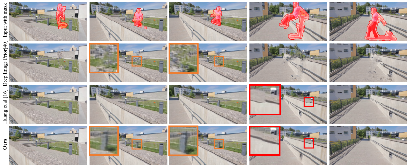
Figure 1: Video inpainting results for the ‘parkour’ sequence. Our video-based internal learning framework enables much more coherent video inpainting results compared to the frame-based baseline [40] ($2^{nd}$ row), even for content unseen in multiple frames (orange box). As a network-based synthesis framework, our method can employ natural image priors to avoid shape distortions, which often occur in patch-based methods such as  [16] ($3^{rd}$ row) for challenging videos (red box).

Video inpainting is the problem of synthesizing plausible visual content within a missing region (‘hole’); for example, to remove unwanted objects. Inpainting is fundamentally ill-posed; there is no unique solution for the missing content. Rather, the goal is to generate visually plausible content that is coherent in both space and time. Priors play a critical role in expressing these constraints. Patch-based optimization methods  [16, 27, 33, 44] effectively leverage different priors such as patch recurrence, total variation, and motion smoothness to achieve state-of-the-art video inpainting results. These priors, however, are mostly hand-crafted and often not sufficient to capture natural image priors, which often leads to distortion in the inpainting results, especially for challenging videos with complex motion (Fig.  1). Recent image inpainting approaches  [18, 31, 35, 48] learn better image priors from an external image corpus via a deep neural network, applying the learned appearance model to hallucinate content conditioned upon observed regions. Extending these deep generative approaches to video is challenging for two reasons. First, the coherency constraints for video are much stricter than for images. The hallucinated content must not only be consistent within its own frame, but also be consistent across adjacent frames. Second, the space of videos is orders of magnitude larger than that of images, making it challenging to train a single model on an external dataset to learn effective priors for general videos, as one requires not only a sufficiently expressive model to generate all variations in the space, but also large volumes of data to provide sufficient coverage.

This paper proposes internal learning for video inpainting inspired by the recently proposed ‘Deep Image Prior’ (DIP) for single image generation  [40]. The striking result of DIP is that ‘knowledge’ of natural images can be encoded through a convolutional neural network (CNN) architecture; i.e. the network structure rather than actual filter weights. The translation equivariance of CNN enables DIP to exploit the internal recurrence of visual patterns in images  [37], in a similar way as the classical patch-based approaches  [19] but with more expressiveness. Furthermore, DIP does not require an external dataset and therefore suffers less from the aforementioned exponential data problem. We explore this novel paradigm of DIP for video inpainting as an alternative to learning priors from external datasets.

Our core technical contribution is the first internal learning framework for video inpainting. Our study establishes the significant result that it is possible to internally train a single frame-wise generative CNN to produce high quality video inpainting results. We report on the effectiveness of different strategies for internal learning to address the fundamental challenge of temporal consistency in video inpainting. Therein, we develop a consistency-aware training strategy based on joint image and flow prediction. Our method enables the network to not only capture short-term motion consistency but also propagate the information across distant frames to effectively handle long-term consistency. We show that our method, whilst trained internally on one (masked) input video without any external data, can achieve state-of-the-art video inpainting result. As a network-based framework, our method can incorporate natural image priors learned from CNN to avoid shape distortions which occur in patch-based methods. (Fig.  1)

A key challenge in extending DIP to video is to ensure temporal consistency; content should be free from visual artifacts and exhibit smooth motion (optical flow) between adjacent frames. This is especially challenging for video inpainting (e.g. versus video denoising) due to the reflexive requirements of pixel correspondence over time to generate missing content, as well as such correspondence to enforce temporal smoothness of that content. We break this cycle by jointly synthesizing content in both appearance and motion domains, generating content through an Encoder-Decoder network that exploits DIP not only in the visual domain but also in the motion domain. This enables us to jointly solve the inpainted appearance and optical flow field – maintaining consistency between the two. We show that simultaneous prediction of both appearance and motion information not only enhances spatial-temporal consistency, but also improves visual plausibility by better propagating structural information within larger hole regions.

2 Related Work

Image/Video Inpainting. The problem of image inpainting/completion [3] has been studied extensively, with classical approaches focusing on patch-based non-parametric optimization [2, 11, 12, 14, 15, 23, 26, 28, 39, 46] as well as more recent work using deep generative neural networks [18, 31, 35, 47, 48]. On the other hand, the video inpainting problem has received far less attention from research community. Most existing video inpainting methods build on patch-based synthesis with spatial-temporal matching [16, 27, 33, 44] or explicit motion estimation and tracking [1, 6, 8, 9]. Very recently, deep convolutional networks have been used to directly inpaint holes in videos and achieve promising results [24, 41, 45], leveraging large external video corpus for training along with specialized recurrent frameworks to model spatial-temporal coherence. Different from their works, we explore the orthogonal direction of learning-based video inpainting by investigating an internal (within-video) learning approach. Video inpainting has also been used as a self-supervised task for deep feature learning [32] which has a different goal from ours.

Internal Learning. Our work is inspired by the recent ‘Deep Image Prior’ (DIP) work by Ulyanov et al. [40] which shows that a static image may be inpainted by a CNN-based generative model trained directly on the non-hole region of the same image with a reconstruction loss. The trained model encodes the visible image contents with white noise, which at the same time enables the synthesis of plausible texture in the hole region. The idea of internal learning has also been shown effective in other application domains, such as image super-resolution  [37], semantic photo manipulation  [4] and video motion transfer  [5]. Recently, Gandelsman et al. [7] further proposes ‘Double-DIP’ for unsupervised image decomposition by reconstructing different layers with multiple DIP. Their framework can also be applied for video segmentation. In this paper, we extend a single DIP to video and explore the effective internal learning strategies for video inpainting.

Flow Guided Image/Video Synthesis. Only encoding frames with a 2D CNN is insufficient to maintain the temporal consistency of a video. Conventionally, people have used optical flow from input source videos as guidance to enhance the temporal consistency of target videos in various video processing tasks such as denoising [20], super-resolution [17], frame interpolation [21], and style transfer [10]. Our work incorporates the temporal consistency constraint of inpainted area by jointly generating images and flows with a new loss function.

3 Video Inpainting via Internal Learning

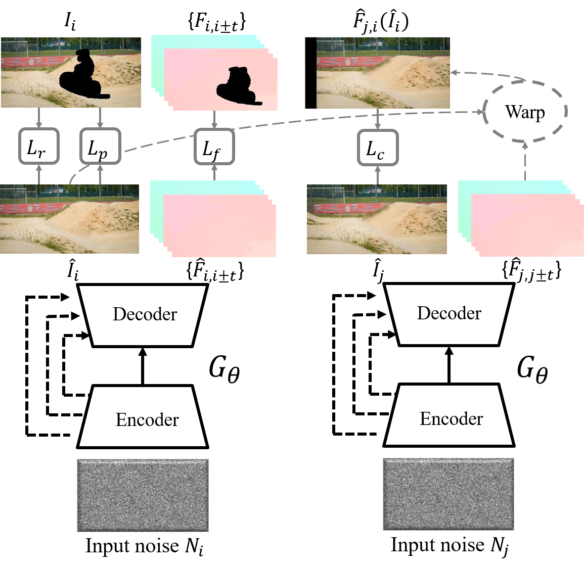
Figure 2: Overview of our video inpainting framework. Given the input random noise $N_{i}$ for each individual frame, a generative network $G_{\theta}$ is used to predict both frame $\hat{I}_{i}$ and optical flow maps $\hat{F}_{i,i\pm t}$. $G_{\theta}$ is trained entirely on the input video (with holes) without any external data, optimizing the combination of the image generation loss $L_{r}$, perceptual loss $L_{p}$, flow generation loss $L_{f}$ and consistency loss $L_{c}$.

The input to video inpainting is a (masked) video sequence $\bar{V}=\{I_{i}\odot M_{i}\}_{i=1..T}$ where $T$ is the total number of frames in the video. $M_{i}$ is the binary mask defining the known regions in each frame $I_{i}$ (1 for the known regions, and 0 otherwise). $\odot$ denotes the element-wise product. Let $I^{*}_{i}$ denote the desired version of $I_{i}$ where the masked region is filled with the appropriate content. The goal in video inpainting is to recover $V^{*}=\{I^{*}_{i}\}_{i=1..T}$ from $\bar{V}$.

In this work, we approach video inpainting with an internal learning formulation. The general idea is to use $\bar{V}$ as the training data to learn a generative neural network $G_{\theta}$ to generate each target frame $I^{*}_{i}$ from a corresponding noise map $N_{i}$. The noise map $N_{i}$ has one channel and shares the same spatial size with the input frame. We sample the input noise maps independently for each frame and fix them during training. Once trained, $G_{\theta}$ can be used to generate all the frames in the video to produce the inpainting results.

$$\vspace{-1mm}I^{*}_{i}=G_{\theta^{*}}(N_{i})\vspace{-2mm}$$ (1)

​​where $\theta$ denotes the network parameters which are optimized during the training process. We implement $G_{\theta}$ as an Encoder-Decoder architecture with skip connections. For each input video, we train an individual model from scratch.

One may concern that a generative model $G_{\theta}$ defined in this way would be too limited for the task of video inpainting as it does not contain any temporal modeling structure required for video generation, e.g. recurrent prediction, attention, memory modeling, etc. In this paper, however, we intentionally keep this extreme form of internal learning and focus on exploring appropriate learning strategies to unleash its potential to perform the video inpainting task. In this section, we discuss our training strategies to train $G_{\theta}$ such that it can generate plausible $V^{*}$.

3.1 Loss Functions

Let $\hat{I}_{i}=G_{\theta}(N_{i})$ be the network output at frame $i$. We define a loss function $L$ at each frame prediction $\hat{I}_{i}$ and accumulate the loss over the whole video to obtain the total loss to optimize the network parameters during training.

$$L=\omega_{r}L_{r}+\omega_{f}L_{f}+\omega_{c}L_{c}+\omega_{p}L_{p}$$ (2)

where $L_{r}$, $L_{f}$, $L_{c}$, and $L_{p}$ denote the image generation loss, flow generation loss, consistency loss, and perceptual loss, respectively. The weights are empirically set as $\omega_{r}{=}1$, $\omega_{f}{=}0.1$, $\omega_{c}{=}1$, $\omega_{p}{=}0.01$ and fixed in all of our experiments. We define each individual loss term as follows:

Image Generation Loss. In the context of image inpainting,  [40] employs the $L_{2}$ reconstruction loss defined on the known regions of the image. Our first attempt to explore internal learning for video inpainting is to define a similar generation loss on each predicted frame.

$$L_{r}(\hat{I_{i}})=\parallel M_{i}\odot\big{(}\hat{I_{i}}-I_{i}\big{)}\parallel^{2}_{2}$$ (3)

Flow Generation Loss. Image generation loss enables the network to reconstruct individual frames, but fails to capture the temporal consistency across frames. Therefore, it is necessary to allow information to be propagated across frames. Our key idea is to encourage the network to learn such propagation mechanism during training. We first augment the network to jointly predict the color and flow values at each pixel: $(\hat{I}_{i},\hat{F}_{i,j})=G_{\theta}(N_{i})$, where $\hat{F}_{i,j}$ denotes the predicted optical flow from frame $i$ to frame $j$ (Fig. 2). To increase the robustness and better capture long-term temporal consistency, our network is designed to jointly predict flow maps with respect to 6 adjacent frames of varying temporal directions and ranges: $j\in\{i\pm 1,i\pm 3,i\pm 5\}$. We define the flow generation loss similarly as the image generation loss to encourage the network to learn the ‘flow priors’ from the known regions:

$$L_{f}(\hat{F}_{i,j})=\parallel O_{i,j}\odot M^{f}_{i,j}\odot\big{(}\hat{F}_{i,j}-F_{i,j}\big{)}\parallel^{2}_{2}.$$ (4)

The known flow $F_{i,j}$ is estimated using PWC-NET [38] from the original input frame $I_{i}$ to $I_{j}$, which also estimates the occlusion map $O_{i,j}$ through the forward-backward consistency check. $M^{f}_{i,j}=M_{i}\cap M_{j}(F_{i,j})$ represents the reliable flow region computed as the intersection of the aligned masks of frame $i$ and $j$.

Consistency Loss. With the network jointly predicts images and flows, we define the image-flow consistency loss to encourage the generated frames and the generated flows to constrain each other: the neighboring frames should be generated such that they are consistent with the predicted flow between them.

$$L_{c}(\hat{I}_{j},\hat{F}_{i,j})=\parallel(1-M^{f}_{i,j})\odot\big{(}\hat{I}_{j}(\hat{F}_{i,j})-\hat{I}_{i}\big{)}\parallel^{2}_{2}$$ (5)

where $\hat{I}_{j}(\hat{F}_{i,j})$ denotes the warped version of the generated frame $\hat{I}_{j}$ using the generated flow $\hat{F}_{i,j}$ through backward warping. We constrain this loss only in the hole regions using the inverse mask $1{-}M^{f}_{i,j}$ to encourage the training to focus on propagating information inside the hole. We find this simple and intuitive loss term allows the network to learn the notion of flow and leverage it to propagate training signal across distant frames (as illustrated in Fig. 3).

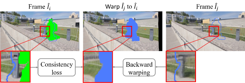
Figure 3: Effectiveness of consistency loss. By warping the predicted frame $\hat{I_{j}}$ into frame $\hat{I_{i}}$, part of the hole region in $\hat{I_{j}}$ can be spatially matched to the visible regions in $\hat{I_{i}}$ (red boxes). This not only provides useful training signal to constrain the inpainting of that region in $\hat{I_{j}}$, but also effectively propagates the content in the visible regions from one frame into the hole regions of its neighboring frames.

Perceptual Loss. To further improve the frame generation quality, we incorporate the popular perceptual loss, defined according to the similarity on extracted feature maps from the pre-trained VGG16 model [22].

$$L_{p}(\hat{I_{i}})=\Sigma_{k\in K}\parallel\psi_{k}(M_{i})\odot\big{(}\phi_{k}(\hat{I_{i}})-\phi_{k}(I_{i})\big{)}\parallel^{2}_{2}$$ (6)

where $\phi_{k}(I_{i})$ denotes the feature extracted from $I_{i}$ using the $k^{th}$ layer of the pre-trained VGG16 network, $\psi_{k}(M_{i})$ denotes the resized mask with the same spatial size as the feature map. This perceptual loss has been used to improve the visual sharpness of generated images [22, 30, 34, 49]. We use 3 layers $\{\mbox{relu}1\_2,\mbox{relu}2\_2,\mbox{relu}3\_3\}$ to define our perceptual loss.

3.2 Network Training

While the standard stochastic training works reasonably, we use the following curriculum-based training procedure during network optimization: Instead of using pure random frames in one batch, we pick $N$ frames which are consecutive with a fixed frame interval of $t$ as a batch. While training with the batch, the flow generation loss and consistency loss are computed only using the corresponding flows ($F_{i,i\pm t}$). We find this helps propagate the information more consistently across the frames in the batch. In addition, inspired by DIP, we perform the parameter update for each batch multiple times continuously, with one forward pass and one back-propagation each time. This allows the network to be optimized locally until the image and flow generation reach their consistent state. We find that using 50-100 updates per batch gives the best performance through experiments of hyper-parameter tuning.

3.3 Implementation Details

We implement our method using PyTorch and run our experiments on a single NVIDIA TITAN Xp GPU. We initialize the model weights using the initialization method described in  [29] and use Adam  [25] with the learning rate of 0.01 and batch size of 5 during training.

Our network is implemented as an Encoder-Decoder architecture with skip connections, which is found to perform well for image inpainting  [40]. The details of the network architecture is provided in the supplementary material.

4 Experiments

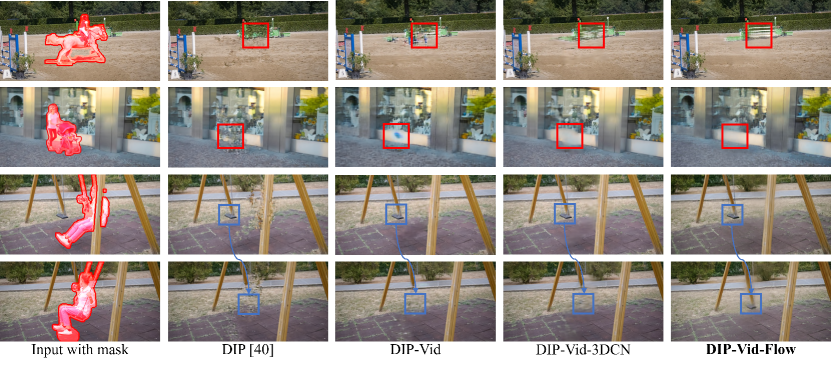
Figure 4: Result comparison between different internal learning frameworks (videos provided in [16]). Frame-wise DIP tends to copy textures from known regions, generating incoherent structures. Optimizing over the whole video (DIP-Vid and DIP-Vid-3DCN) improves the visual quality but does not capture temporal consistency well (blue boxes in $3^{rd}$ and $4^{th}$ rows). Our proposed consistency loss (DIP-Vid-Flow) improves long-term temporal consistency.

We evaluate our method on a variety of real-world videos used in previous works, including 28 videos collected by Huang et al. [16] from the DAVIS dataset [36], and 13 videos collected from  [8, 9, 33].

To facilitate quantitative evaluation, we create an additional dataset in which each video has both the foreground masks and the ground-truth background frames. We retrieved 50 background videos from Flickr using different keywords to cover a wide range of scenes and motion types. We randomly select a segment of 60 frames for each video and compose each video with 5 masks randomly picked from DAVIS. This results in 250 videos with real video background and real object masks, which is referred as our Composed dataset.

4.1 Ablation Study

We first compare the video inpainting quality between different internal learning approaches. In particular, we compare our final method, referred to as DIP-Vid-Flow, with the following baselines:

DIP: This baseline directly applies the ‘Deep Image Prior’ framework [40] to video in a frame-by-frame manner.

DIP-Vid: This is our framework when the model is trained only using the image generation loss (Eq. 3).

DIP-Vid-3DCN: Besides directly using the DIP framework in [40] with pure 2D convolution, we modify the network to use 3D convolution and apply the image generation loss.

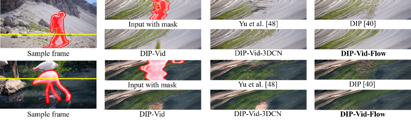
Figure 5: Temporal consistency comparison (videos provided in [16]). We stack the pixels in a fixed row (indicated by the yellow line) from all the frames of the video. Our full model (DIP-Vid-Flow) shows the smoothest temporal transition.

We evaluate the video inpainting quality in terms of frame-wise visual plausibility, temporal consistency and reconstruction accuracy on our Composed dataset for which the ‘ground-truth’ background videos are available. For visual plausibility, we compute the Fréchet Inception Distance (FID) score [13] of each inpainted frame independently against the full collection of ground-truth frames and aggregate the value over the whole video. For temporal consistency, we use the consistency metric introduced in [10]. For each $50{\times}50$ patch sampled in the hole region at frame $t$ we search within the spatial neighborhood of 20 pixels at time $t+1$ for the patch that maximizes the peak signal-to-noise ratio (PSNR) between the two patches. We compute the average PSNR from all the patches as the metric. Similar metric is also computed using SSIM [43]. For reconstruction accuracy, we compute the standard PSNR and SSIM on each frame, accumulate the metrics over each video, and report the average performance for each method.

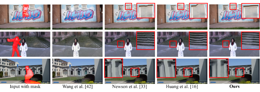
Figure 6: Video inpainting results on the videos provided in [16] ($1^{st}$ row) and  [8]($2^{nd}$ row) as well as our Composed dataset ($3^{rd}$). Our results are less prone to shape distortion compared to those generated by patch-based methods.

Method	FID	Consistency	PSNR/SSIM
DIP  [40]	22.3	18.8/0.532	25.2/.926
DIP-Vid	16.1	23.6/0.768	28.7/.956
DIP-Vid-3DCN	12.1	26.7/0.871	30.9/.966
DIP-Vid-Flow	10.4	28.1/0.895	32.1/.969

Table 1: Ablation Study. Visual plausibility (FID), temporal consistency (PSNR/SSIM), and reconstruction accuracy (PSNR/SSIM) on our Composed dataset. Our full model outperforms all the baselines in all the metrics.

Tab. 1 shows the results of different methods. For all metrics, the video-wise methods significantly improve over the frame-wise DIP method. Incorporating temporal information can further improve the results. Explicitly modeling the temporal information in the form of flow prediction leads to the best results.

Fig. 4 shows some visual examples. DIP often borrows textures from known regions to fill in the hole, generating incoherent structures in many cases. Training the model over the whole video (DIP-Vid) allows the network to generate better structures, improving the visual quality in each frame. Using 3D convolution tends to constrain the large hole better than 2D due to the larger context provided by the spatial-temporal volume. The result, however, tends to be more blurry and distorted as it is in general very challenging to model the space of spatial-temporal patches. Training the model with our full internal learning framework allows the information to propagate properly across frames which constrains the hole regions with the right information.

Fig. 5 visualizes temporal consistency of different video inpainting results on two video sequences.We visualize the video content at a fixed horizontal stride across the whole video. Note that the strides cut through the hole regions in many frames. As the video progresses, the visualization from a good video inpainting result should appear smooth. Applying the image inpainting methods [40, 48] result in inconsistency between the hole regions and non-hole regions across the video. DIP-Vid and DIP-Vid-3DCN result in smoother visualizations compared to DIP yet still exhibit inconsistent regions while our full model gives the smoothest visualization, indicating high temporal consistency.

4.2 Video Inpainting Performance

We compare the video inpainting performance of our internal-learning method with different state-of-the-art inpainting methods, including the inpainting results obtained from one state-of-the art image inpainting method by Yu et al. [48], Vid2Vid (Wang et al. [42]) model trained on video inpainting data, and two state-of-the-art video inpainting methods by Newson et al. [33] and Huang et al. [16]. For Vid2Vid, we train the model on a different composed dataset created for video inpainting. The training set containing 1000 videos of 30-frames each is constructed with the same procedure used for our Composed dataset.

	All	Complex	Simple
Yu et al. [48]	24.9/.929	24.7/.926	25.1/.931
Wang et al. [42]	26.0/.914	25.3/.908	26.6/.920
Newson et al. [33]	30.6/.962	30.9/.963	30.4/.960
Huang et al. [16]	32.3/.971	31.6/.968	33.0/.974
Ours	32.1/.969	31.9/.970	32.2/.968

Table 2: Quantitative Evaluation. PSNR/SSIM on our Composed dataset as well as its two partitions. Our method produces more accurate video inpainting results than most of the existing methods. Our method performs favorably for challenging videos with complex motion.

For quantitative evalution, we report PSNR and SSIM on our Composed dataset in Tab. 2. The results show that our method produces more accurate video inpainting results than most of the existing methods, except for Huang et al. [16]. Fig. 6 shows some visual examples of the inpainted frames from different methods. Please refer to our supplementary video for more results.

Interestingly, we observe that our results complement those of the patch-based methods when videos have more complex background motion or color/lighting changes. Patch-based methods rely on explicit patch matching and flow tracking during synthesis, which often fail when the appearance or motion varies significantly. This leads to distorted shapes inconsistent with the known regions (see Fig. 6 for visual examples). On the other hand, our network-based synthesis tends to capture better natural image priors and handles those scenarios more robustly.

To further understand this complementary behavior, we separate our Composed dataset into two equal partitions according to video complexity defined by the metric as the sum of two terms: the standard deviation of average pixel values across the frames, which measures the appearance change; and the mean of the flow gradient magnitude, which reflects the motion complexity. We report PSNR and SSIM for these two partitions in Tab. 2, as well as in Fig. 7, where we plot the average performance of videos whose complexity metric is above certain threshold. It shows that our method tends to perform slightly better compared with patch-based methods when the video complexity increases.

Figure 7: Comparison between our method and the state-of-the-art video inpainting method [16]. We plot the average performance of videos whose complexity metric are above the threshold in x-axis. Our method performs consistently better when the appearance and motion gets more complex.

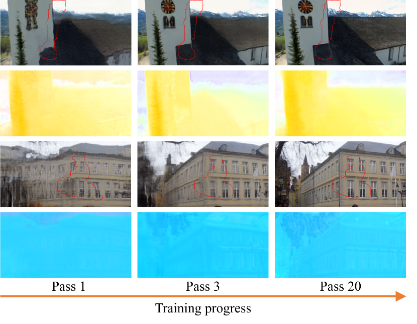
Figure 8: Intermediate results during training. Generated frames: red curve outlines the hole region. Generated flow maps (forward flow with range 1): hue denotes the flow orientation, value denotes the magnitude. As the training progresses, the model captures more accurate texture and motion (the flow map becomes smoother and more consistent with the actual video scene).

Fig. 8 shows our generated frames and flow maps during training process. After one pass through all the frames, our model is able to reconstruct the global structure of the frames. Ghosting effect is usually observed at this stage because the mapping from noise to image is still not well established for individual frames. During the next several passes, the model gradually learns more texture details of the frames, both inside and outside the hole region. The inpainting result is generally good after just a few passes through the whole video. In practice, we keep training longer to further improve the long-term temporal consistency, since it takes more iterations for the contents from distant frames to come into play via the consistency loss. In Fig. 8, we observe that the predicted flow in the hole region is coherent with their neighboring content, indicating effective flow inpainting. We also note that the predicted flow orientation (represented by the hue in the visualized flow maps) is also consistent with the camera motion, thereby serving as a guidance for the image generation.

5 Discussion

In this section, we visualize the encoded latent feature and investigate the influence of input window length to further understand our model.

5.1 Visualization of Encoded Latent Feature

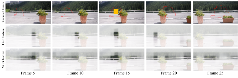
Figure 9: Visualization of feature similarity of our model compared with VGG. A higher opacity patch indicates higher feature similarity. Our learned feature is able to track the exact patch instead of only searching for visually similar patches.

Recall that our generator $G_{\theta}$ has an Encoder-Decoder structure that encodes random noise to latent features and decodes the features to generate image pixels. To better understand how the model works, it is helpful to inspect the feature learned by the encoder. In Fig. 9, we visualize the feature similarity between a reference patch and all the other patches from neighboring locations and other frames. Specifically, we select a reference patch from the middle frame with patch size 32x32 matching the receptive field of the encoder, and calculate the cosine similarity between the features of the reference and other patches. The feature vector of a patch is given by the neuron responses at the corresponding 1x1 spatial location of the feature map. The patch similarity map is shown on the middle frame as well as 4 nearby frames, encoded in the alpha channel. A higher opacity patch indicates a higher feature similarity. As a comparison, we show the similarity map calculated with both our learned feature (middle row) and VGG16-pool5 feature (bottom row). It can be observed from the example in Fig. 9 that the most similar patches identified by our learned feature are located on the exact same object across a long range of frames; VGG feature can capture general visual similarity but fails to identify the same object instance. This interesting observation provides some indication that certain video specific features have been learned during the internal learning process.

5.2 Influence of Window Length

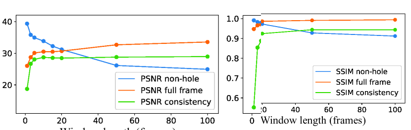
Figure 10: Influence of window length: As the window length increases, the reconstruction quality in the non-hole region decreases. However, the overall inpainting quality improves, indicating the improvement in generalization in the hole regions as more frames become available.

In our framework, the input video can be considered as the training data with which the inpainting generative network is trained. To investigate how the inpainting performance is affected by the input window length, we perform an experiment on a subset of 10 videos randomly selected from our Composed dataset. We divide each video into clips of window length $k$ and apply our inpainting method on each clip independently. We experiment with different window length $k\in\{1,3,5,10,15,25,50,100\}$. We plot the average PSNR and SSIM scores of both generated non-hole region and full frame (the generated hole fused with the input non-hole region), as well as the consistency metric introduced in Sec. 4.1 under each setting in Fig. 10.

Interestingly, while the overall inpainting quality improves as $k$ increases, the reconstruction quality in the non-hole region decreases. This indicates overfitting when training on limited data. In fact, when $k{=}1$, it reduces to running DIP frame-wise which gives the best reconstruction quality on the non-hole region. The fact that our method achieves better inpainting results with larger window length indicates the capability of the model in leveraging distant frames to generate better results in the hole region.

5.3 Limitation and Future Work

As is the case with DIP [40] and many other back-propagation based visual synthesis system, long processing time is the main limitation of our method. It often takes hours to train an individual model for each input video. Our method can fail when the hole is large and has little motion relative to the background. In those cases, there is too little motion to propagate the content across frames. Nevertheless, the value of our work lies in exploring the possibilities of internal learning on video inpainting and identifying its strength that complements other learning-based methods relying on external training data. In future work, we plan to further investigate how to combine representations learned internally with externally trained models to enable powerful learning systems.

It remains an open question that, in the context of internal learning, what network structure can best serve as a prior to represent video sequence data. In this work, we have intentionally restricted the network to a 2D CNN structure to study the capability of such a simple model in encoding temporal information. In future work, we plan to study more advanced architectures with explicit in-network temporal modeling, such as recurrent networks and sequence modeling in Vid2Vid [42].

6 Conclusion

In this paper, we introduce a novel approach for video inpainting based on internal learning. In extending Deep Image Prior  [40] to video, we explore effective strategies for internal learning to address the fundamental challenge of temporal consistency in video inpainting. We propose a consistency-aware training framework to jointly generate both appearance and flow, whilst exploiting these complementary modalities to ensure mutual consistency. We demonstrate that it is possible for a regular image-based generative CNN to achieve coherent video inpainting results, while optimizing directly on the input video without reliance upon an external corpus of visual data. With this work, we hope to attract more research attention to the interesting direction of internal learning, which is complementary to the mainstream large-scale learning approaches. We believe combining the strengths from both directions can potentially lead to better learning methodologies.

Acknowledgments This project is supported in part by the Brown Institute for Media Innovation. We thank Flickr users Horia Varlan, tyalis_2, Andy Tran and Ralf Kayser for their permissions to use their videos in our experiments.

Appendix A Network Architecture

In our experiments, we use two different networks. Our 2D baselines (DIP and DIP-Vid) and our final model (DIP-Vid-Flow) share the same Encoder-Decoder architecture. Our 3D baseline (DIP-Vid-3DCN) uses a modified version with 3D convolution. The source code is available at our project website https://cs.stanford.edu/~haotianz/publications/video_inpainting/.

A.1 2D Network

Encoder The Encoder consists of 12 convolution layers. Every two consecutive layers form a block, where the two layers have the same number of channels. The first layer in each block uses the stride of 2 to reduce the spatial resolution. All the convolution layers use the filter size of 5. The number of channels for each layer is shown below.

C16-C16-C32-C32-C64-C64-C128-C128-C128-C128-C128-C128

Decoder The Decoder also consists of 12 convolution layers in 6 blocks. One Nearest-neighbor upsampling layer is added to the beginning of each block. All the convolution layers use the filter size of 3. The number of channels for each layer are symmetric to those in the Encoder.

Skip Connection A skip connection is added from the beginning of the $i$ th block of the Encoder to the beginning of the $(n-i)$ th block (after the upsampling layer) of the Decoder. All skip connections use one convolution layer with 4 channels and filter size of 1.

Final Layer For DIP and DIP-Vid, the final layer only contains a convolution layer with 3 channels followed by a sigmoid to generate the final image. For DIP-Vid-Flow, a flow generation branch is added parallel to the image generation branch, which contains a convolution layer with 12 channels, corresponding to 6 different flow maps of temporal range 1, 3, 5 in both forward and backward directions.

All the convolution layers except those in the final layer are followed by a Batch-Norm layer and a LeakyReLU layer with slope 0.2.

A.2 3D Network

Our 3D version of the network shares the same structure with the 2D version except all the 2D convolution layers are replaced with 3D convolution layers. We also keep all the number of channels and filter size as the same as our 2D version. For the added $3^{rd}$ dimension, we use the filter size of 3 for the Encoder and the Decoder and the filter size of 1 for the skip connections.

Appendix B Network Input

As mentioned in the main paper, we sample the input noise maps independently for each frame and fix them during training. The noise map has one channel and shares the same spatial size with the input frame. Each noise map is filled with uniform noise between 0 and 0.1. For our 2D network, we feed input noise maps as a 2D batch of dimension $N\times 1\times H\times W$, where N is the batch size. For our 3D network, we transfer the 2D batch into a 3D batch of dimension $1\times 1\times N\times H\times W$, where $N$ becomes the size of the $3^{rd}$ dimension with batch size of 1. In all of our experiments, frames are resized and cropped to $384\times 192$.

Appendix C Network Training

In this section, we describe the training details for all the baselines and our final model.

C.1 DIP

We train a DIP model for each frame independently. Due to the destabilization issue mentioned in the original paper  [40], we run optimization on each frame for 5k iterations and save the result every 100 iterations. The intermediate result with the lowest loss is chosen as the final result.

C.2 DIP-Vid

We train a single DIP model on the entire video. In each epoch, we randomly pick $N$ consecutive frames as a training batch to enumerate all the possible batch permutations. Inspired by the training procedure used in DIP, we run optimization on the selected batch for $M$ iterations before moving to the next batch. After training for $E$ epochs, we run one inference using the trained model to get the final inpainting results. Only the image generation loss is applied in this baseline. The destabilization issue is also observed in this method, but considerably rare compared to DIP.

C.3 DIP-Vid-3DCN

All the settings are as the same as DIP-Vid, except for replacing the 2D network with the 3D version.

C.4 DIP-Vid-Flow

In our final model, we need to generate both images and flows. We randomly pick N frames which are consecutive with a fixed frame interval of t as a batch, $t\in\{1,3,5\}$. We do not use intervals larger than 5 due to the increasing error in estimated flows. We run optimization on the batch with all the image and flow related loss (See Sec3.1 in our main paper), but only using forward or backward flow at interval $t$ for $M$ iterations. Optimizing flows in both directions at the same time is observed to cause artifacts in the results occasionally, potentially due to the conflict in the flows. We select batches by enumerating all the possible permutations and finish training after $E$ epochs on the whole video.

We use $N=5$, $M=100$ and $E=20$ in all of our experiments.

References

- [1] Mahmoud Afifi, Khaled F Hussain, Hosny M Ibrahim, and Nagwa M Omar. Fast video completion using patch-based synthesis and image registration. In 2014 International Symposium on Intelligent Signal Processing and Communication Systems (ISPACS), pages 200–204. IEEE, 2014.
- [2] Connelly Barnes, Eli Shechtman, Adam Finkelstein, and Dan B Goldman. Patchmatch: A randomized correspondence algorithm for structural image editing. ACM Transactions on Graphics (ToG), 28(3):24, 2009.
- [3] Connelly Barnes and Fang-Lue Zhang. A survey of the state-of-the-art in patch-based synthesis. Computational Visual Media, 3(1):3–20, 2017.
- [4] David Bau, Hendrik Strobelt, William Peebles, Jonas Wulff, Bolei Zhou, Jun-Yan Zhu, and Antonio Torralba. Semantic photo manipulation with a generative image prior. ACM Transactions on Graphics (Proceedings of ACM SIGGRAPH), 38(4), 2019.
- [5] Caroline Chan, Shiry Ginosar, Tinghui Zhou, and Alexei A Efros. Everybody dance now. arXiv preprint arXiv:1808.07371, 2018.
- [6] Mounira Ebdelli, Olivier Le Meur, and Christine Guillemot. Video inpainting with short-term windows: application to object removal and error concealment. IEEE Transactions on Image Processing, 24(10):3034–3047, 2015.
- [7] Yossi Gandelsman, Assaf Shocher, and Michal Irani. ”double-dip”: Unsupervised image decomposition via coupled deep-image-priors. In The IEEE Conference on Computer Vision and Pattern Recognition (CVPR), 6 2019.
- [8] Miguel Granados, Kwang In Kim, James Tompkin, Jan Kautz, and Christian Theobalt. Background inpainting for videos with dynamic objects and a free-moving camera. In European Conference on Computer Vision, pages 682–695. Springer, 2012.
- [9] Miguel Granados, James Tompkin, K Kim, Oliver Grau, Jan Kautz, and Christian Theobalt. How not to be seen—object removal from videos of crowded scenes. In Computer Graphics Forum, volume 31, pages 219–228. Wiley Online Library, 2012.
- [10] Agrim Gupta, Justin Johnson, Alexandre Alahi, and Li Fei-Fei. Characterizing and improving stability in neural style transfer. In Proceedings of the IEEE Conference on Computer Vision and Pattern Recognition, pages 4067–4076, 2017.
- [11] James Hays and Alexei A Efros. Scene completion using millions of photographs. ACM Transactions on Graphics (TOG), 26(3):4, 2007.
- [12] Kaiming He and Jian Sun. Image completion approaches using the statistics of similar patches. IEEE transactions on pattern analysis and machine intelligence, 36(12):2423–2435, 2014.
- [13] Martin Heusel, Hubert Ramsauer, Thomas Unterthiner, Bernhard Nessler, and Sepp Hochreiter. Gans trained by a two time-scale update rule converge to a local nash equilibrium. In Advances in Neural Information Processing Systems, pages 6626–6637, 2017.
- [14] Joo Ho Lee, Inchang Choi, and Min H Kim. Laplacian patch-based image synthesis. In Proceedings of the IEEE Conference on Computer Vision and Pattern Recognition, pages 2727–2735, 2016.
- [15] Jia-Bin Huang, Sing Bing Kang, Narendra Ahuja, and Johannes Kopf. Image completion using planar structure guidance. ACM Transactions on graphics (TOG), 33(4):129, 2014.
- [16] Jia-Bin Huang, Sing Bing Kang, Narendra Ahuja, and Johannes Kopf. Temporally coherent completion of dynamic video. ACM Transactions on Graphics (TOG), 35(6):196, 2016.
- [17] Yan Huang, Wei Wang, and Liang Wang. Video super-resolution via bidirectional recurrent convolutional networks. IEEE transactions on pattern analysis and machine intelligence, 40(4):1015–1028, 2017.
- [18] Satoshi Iizuka, Edgar Simo-Serra, and Hiroshi Ishikawa. Globally and locally consistent image completion. ACM Transactions on Graphics (ToG), 36(4):107, 2017.
- [19] Daniel Glasner Shai Bagon Michal Irani. Super-resolution from a single image. In Proceedings of the IEEE International Conference on Computer Vision, Kyoto, Japan, pages 349–356, 2009.
- [20] Hui Ji, Chaoqiang Liu, Zuowei Shen, and Yuhong Xu. Robust video denoising using low rank matrix completion. In 2010 IEEE Computer Society Conference on Computer Vision and Pattern Recognition, pages 1791–1798. IEEE, 2010.
- [21] Huaizu Jiang, Deqing Sun, Varun Jampani, Ming-Hsuan Yang, Erik Learned-Miller, and Jan Kautz. Super slomo: High quality estimation of multiple intermediate frames for video interpolation. In Proceedings of the IEEE Conference on Computer Vision and Pattern Recognition, pages 9000–9008, 2018.
- [22] Justin Johnson, Alexandre Alahi, and Li Fei-Fei. Perceptual losses for real-time style transfer and super-resolution. In European Conference on Computer Vision, pages 694–711. Springer, 2016.
- [23] Nima Khademi Kalantari, Eli Shechtman, Soheil Darabi, Dan B Goldman, and Pradeep Sen. Improving patch-based synthesis by learning patch masks. In 2014 IEEE International Conference on Computational Photography (ICCP), pages 1–8. IEEE, 2014.
- [24] Dahun Kim, Sanghyun Woo, Joon-Young Lee, and In So Kweon. Deep video inpainting. In Proceedings of the IEEE Conference on Computer Vision and Pattern Recognition, pages 5792–5801, 2019.
- [25] Diederik P Kingma and Jimmy Ba. Adam: A method for stochastic optimization. arXiv preprint arXiv:1412.6980, 2014.
- [26] Nikos Komodakis. Image completion using global optimization. In 2006 IEEE Computer Society Conference on Computer Vision and Pattern Recognition (CVPR), volume 1, pages 442–452. IEEE, 2006.
- [27] Thuc Trinh Le, Andrés Almansa, Yann Gousseau, and Simon Masnou. Motion-consistent video inpainting. In 2017 IEEE International Conference on Image Processing (ICIP), pages 2094–2098. IEEE, 2017.
- [28] Olivier Le Meur, Mounira Ebdelli, and Christine Guillemot. Hierarchical super-resolution-based inpainting. IEEE transactions on image processing, 22(10):3779–3790, 2013.
- [29] Yann A LeCun, Léon Bottou, Genevieve B Orr, and Klaus-Robert Müller. Efficient backprop. In Neural networks: Tricks of the trade, pages 9–48. Springer, 2012.
- [30] Christian Ledig, Lucas Theis, Ferenc Huszár, Jose Caballero, Andrew Cunningham, Alejandro Acosta, Andrew Aitken, Alykhan Tejani, Johannes Totz, Zehan Wang, et al. Photo-realistic single image super-resolution using a generative adversarial network. In Proceedings of the IEEE conference on computer vision and pattern recognition, pages 4681–4690, 2017.
- [31] Guilin Liu, Fitsum A Reda, Kevin J Shih, Ting-Chun Wang, Andrew Tao, and Bryan Catanzaro. Image inpainting for irregular holes using partial convolutions. In Proceedings of the European Conference on Computer Vision (ECCV), pages 85–100, 2018.
- [32] Adithya Reddy Nallabolu. Unsupervised Learning of Spatiotemporal Features by Video Completion. PhD thesis, Virginia Tech, 2017.
- [33] Alasdair Newson, Andrés Almansa, Matthieu Fradet, Yann Gousseau, and Patrick Pérez. Video inpainting of complex scenes. SIAM Journal on Imaging Sciences, 7(4):1993–2019, 2014.
- [34] Simon Niklaus, Long Mai, and Feng Liu. Video frame interpolation via adaptive separable convolution. In Proceedings of the IEEE International Conference on Computer Vision, pages 261–270, 2017.
- [35] Deepak Pathak, Philipp Krahenbuhl, Jeff Donahue, Trevor Darrell, and Alexei A Efros. Context encoders: Feature learning by inpainting. In Proceedings of the IEEE conference on computer vision and pattern recognition, pages 2536–2544, 2016.
- [36] Federico Perazzi, Jordi Pont-Tuset, Brian McWilliams, Luc Van Gool, Markus Gross, and Alexander Sorkine-Hornung. A benchmark dataset and evaluation methodology for video object segmentation. In Proceedings of the IEEE Conference on Computer Vision and Pattern Recognition, pages 724–732, 2016.
- [37] Assaf Shocher, Nadav Cohen, and Michal Irani. “zero-shot” super-resolution using deep internal learning. In Proceedings of the IEEE Conference on Computer Vision and Pattern Recognition, pages 3118–3126, 2018.
- [38] Deqing Sun, Xiaodong Yang, Ming-Yu Liu, and Jan Kautz. Pwc-net: Cnns for optical flow using pyramid, warping, and cost volume. In Proceedings of the IEEE Conference on Computer Vision and Pattern Recognition, pages 8934–8943, 2018.
- [39] Jian Sun, Lu Yuan, Jiaya Jia, and Heung-Yeung Shum. Image completion with structure propagation. ACM Transactions on Graphics (ToG), 24(3):861–868, 2005.
- [40] Dmitry Ulyanov, Andrea Vedaldi, and Victor Lempitsky. Deep image prior. In Proceedings of the IEEE Conference on Computer Vision and Pattern Recognition, pages 9446–9454, 2018.
- [41] Chuan Wang, Haibin Huang, Xiaoguang Han, and Jue Wang. Video inpainting by jointly learning temporal structure and spatial details. In Proceedings of the AAAI Conference on Artificial Intelligence, volume 33, pages 5232–5239, 2019.
- [42] Ting-Chun Wang, Ming-Yu Liu, Jun-Yan Zhu, Guilin Liu, Andrew Tao, Jan Kautz, and Bryan Catanzaro. Video-to-video synthesis. In Advances in Neural Information Processing Systems, pages 1144–1156, 2018.
- [43] Zhou Wang, Alan C Bovik, Hamid R Sheikh, and Eero P Simoncelli. Image quality assessment: from error visibility to structural similarity. IEEE transactions on image processing, 13(4):600–612, 2004.
- [44] Yonatan Wexler, Eli Shechtman, and Michal Irani. Space-time video completion. In Proceedings of the 2004 IEEE Computer Society Conference on Computer Vision and Pattern Recognition, 2004. CVPR 2004., volume 1, pages I–I. IEEE, 2004.
- [45] Rui Xu, Xiaoxiao Li, Bolei Zhou, and Chen Change Loy. Deep flow-guided video inpainting. In The IEEE Conference on Computer Vision and Pattern Recognition (CVPR), June 2019.
- [46] Zongben Xu and Jian Sun. Image inpainting by patch propagation using patch sparsity. IEEE transactions on image processing, 19(5):1153–1165, 2010.
- [47] Chao Yang, Xin Lu, Zhe Lin, Eli Shechtman, Oliver Wang, and Hao Li. High-resolution image inpainting using multi-scale neural patch synthesis. In Proceedings of the IEEE Conference on Computer Vision and Pattern Recognition, pages 6721–6729, 2017.
- [48] Jiahui Yu, Zhe Lin, Jimei Yang, Xiaohui Shen, Xin Lu, and Thomas S Huang. Generative image inpainting with contextual attention. In Proceedings of the IEEE Conference on Computer Vision and Pattern Recognition, pages 5505–5514, 2018.
- [49] Richard Zhang, Phillip Isola, Alexei A Efros, Eli Shechtman, and Oliver Wang. The unreasonable effectiveness of deep features as a perceptual metric. In Proceedings of the IEEE Conference on Computer Vision and Pattern Recognition, pages 586–595, 2018.