Sparse Canonical Correlation Analysis via Concave Minimization

Abstract

A new approach to the sparse Canonical Correlation Analysis (sCCA) is proposed with the aim of discovering interpretable associations in very high-dimensional multi-view, i.e. observations of multiple sets of variables on the same subjects, problems. Inspired by the sparse PCA approach of Journée et al. (2010), we also show that the sparse CCA formulation, while non-convex, is equivalent to a maximization program of a convex objective over a compact set for which we propose a first-order gradient method. This result helps us reduce the search space drastically to the boundaries of the set. Consequently, we propose a two-step algorithm, where we first infer the sparsity pattern of the canonical directions using our fast algorithm, then we shrink each view, i.e. observations of a set of covariates, to contain observations on the sets of covariates selected in the previous step, and compute their canonical directions via any CCA algorithm. We also introduce Directed Sparse CCA, which is able to find associations which are aligned with a specified experiment design, and Multi-View sCCA which is used to discover associations between multiple sets of covariates. Our simulations establish the superior convergence properties and computational efficiency of our algorithm as well as accuracy in terms of the canonical correlation and its ability to recover the supports of the canonical directions. We study the associations between metabolomics, trasncriptomics and microbiomics in a multi-omic study using MuLe, which is an R package that implements our approach, in order to form hypotheses on mechanisms of adaptations of Drosophila Melanogaster to high doses of environmental toxicants, specifically Atrazine, which is a commonly used chemical fertilizer.

Keywords: sparse CCA, Canonical Correlation Analysis, Multivariate Analysis, Multivariate Learning

1 Introduction

Canonical Correlation Analysis(CCA), Hotelling (1935) , is a powerful set of approaches for analyzing the relationship between two sets of random vectors, and discovering associations between elements of said vectors. Classical CCA is specifically concerned with finding linear combinations of the elements of each random vector such that they are maximally correlated estimated using observations of each random vector on matching subjects/individuals, i.e. different views, of the same latent random vector. In this article, we use the terms view and dataset interchangeably, denoted by $\bm{X}_{i}\in\mathbb{R}^{n\times p_{i}}$, to refer to $n$ observations of a random vector of length $p_{i}$.

CCA has been widely used in various fields of data science and machine learning and has found successful applications in finance, neuro-imaging, computer vision, NLP, social sciences, geography, collaborative filtering, astronomy and a new surge in genomics, especially in recently popular multi-assay genetic/clinical population studies. After its proposition by Hotelling (1935), CCA was first applied in Waugh (1942) where he studied the relationship between the characteristics of wheat and the resulting flour. He demonstrated that desirable wheat is high in texture, density and protein content and low on damaged kernels and foreign materials. Other rather classic applications of CCA include: medical geography, where Monmonier and Finn (1973) showed direct association between the number of hospital beds per capita and physician ratios, socio-medical studies, e.g. Hopkins (1969) studies the relationship between housing and health in Baltimore, education, Dunham and Kravetz (1975) analyzes the association between measures of academic performance in college and exam scores in high school, economics, where Simonson et al. (1983) employs this technique to identify and describe hedging behavior between the asset side and the capital side of the balance sheets of a selection of US. banks, signal processing, e.g. Schell and Gardner (1995) introduces Programmable CCA to design filters to distinguish between desired signal and noise, time-series analysis, e.g. Heij and Roorda (1991) employs CCA for state-space modeling, geography, e.g. Ouarda et al. (2001) perform a regional flood frequency analysis using CCA by investigating the correlation structure between watershed characteristics and flood peaks, medical imaging, e.g. Friman et al. (2001) benefited from CCA in detecting activated brain regions based on physiological parameters such as temporal shape and delay of the hemodynamic response. There are plenty of other examples in the fields of chemistry, e.g. Tu et al. (1989), physics, e.g. Wong et al. (1980), dentistry, e.g. Lindsey et al. (1985) where CCA is utilized to discover complex yet meaningful associations between two sets of variables.

CCA and its variants have also found substantial grounds in modern fields of research such as artificial intelligence and statistical learning, neuro-imaging and human perception, context-based content retrieval, collaborative filtering, dimensionality reduction and feature selection, and spatial and temporal genome-wide association studies. Cao et al. (2015) and Nakanishi et al. (2015) used CCA in the area of Brain Computer Interface(BCI) to recognize the frequency components of target stimuli. In the area of image recognition, Hardoon et al. (2004) use a kernel CCA method to perform content-based image retrieval and learn semantics of multimedia content by combining image and text data. Ogura et al. (2013), Shen et al. (2013), and Wang et al. (2013) have employed CCA and its variants for the purpose of feature selection/extraction/fusion and dimensionality reduction.

Modern Canonical Correlation Analysis algorithms have had a significant surge in genomics esp. multi-omic genetic and environmental studies in the last few years mainly due to fast and efficient genome sequencing and measurement technologies becoming more accessible. Such studies typically involve two or more, usually high-dimensional, omic datasets, e.g. trascriptomic, metabolomic, microbiomic data. An instance of such study is Hyman et al. (2002) where they performed CGH analysis on cDNA microarrays in breast cancer and compared copy number and mRNA expression levels to infer the impact of genomic changes on gene expression. Yamanishi et al. (2003) successfully utilized this method to recognize the operons in Escherichia Coli genome by comparing three datasets corresponding to functional, locational and expression relationships between the genes. Morley et al. (2004), Pollack et al. (2002), Snijders et al. (2017), Orsini et al. (2018), Fang et al. (2016), Rousu et al. (2013), Seoane et al. (2014), Baur and Bozdag (2015), Sarkar and Chakraborty (2015), and Cichonska et al. (2016) are few other notable relevant works.

In the next section we provide an overview of the common approaches, but we first compile the notation used throughout the paper in the subsection below.

2 Notation

Each view, i.e. the observation matrix on random vector $X_{i}(\omega):\Omega\rightarrow\mathbb{R}^{p_{i}}$, is denoted by $\bm{X}_{i}\in\mathbb{R}^{n\times p_{i}}$, $i=1,\ldots,m$. $n$ is reserved to denote the sample size and $p_{i}$ to denote the length of each random vector $X_{i},i=1,\ldots,m$. Canonical directions are denoted by $\bm{z}_{i}\in\mathcal{B}^{p_{i}}$, or $\bm{z}_{i}\in\mathcal{S}^{p_{i}}$, and $\bm{Z}_{i}\in\mathcal{S}_{d}^{p_{i}}$, where $\mathcal{B}=\{\bm{x}\in\mathbb{R}|\|\bm{x}\|_{2}\leq 1\}$ and $\mathcal{S}=\{\bm{x}\in\mathbb{R}|\|\bm{x}\|_{2}=1\}$. $l_{x}(\bm{z})=\|\bm{z}\|_{x}:\mathbb{R}^{p}\rightarrow\mathbb{R}$ denotes any norm function, more specifically $l_{0/1}(\bm{z})=\|\bm{z}\|_{0/1}$, and $\bm{\tau}^{(i)}$ refers to the $i-th$ non-zero element of the vector which is specifically used for the sparsity pattern vector. Sample covariance matrices corresponding to the $i$-th and $j$-th views is denoted by $\bm{C}_{ij}$. We drop the subscript when we only have two views. $max(x,0)$ is also denoted by $[x]_{+}$. We also coin the term accessory variables in Section 5.2 to refer to the variables towards which we direct estimated canonical directions, disregarding their causal roles as covariates or dependent variables. We also use “program” to refer to “optimization programs”.

3 An Overview of Approaches to the CCA Problem

This subsection covers a literature review of Canonical Correlation Analysis, common approaches, and their statistical assumptions and approximations. While linear approaches and especially their regularized extensions are the main focus of this paper, we have also provided an overview of non-linear approaches, e.g. kernelized model of Lai and Fyfe (2000) and DeepCCA of Andrew et al. (2013).

3.1 CCA

Let $X(\omega):\Omega\rightarrow\mathbb{R}^{p}$ be a random vector with covariance matrix $\bm{\Sigma}\in\mathbb{R}^{p\times p}$. Further assume that $\mathbb{E}X=\mathbf{0}$. Now partition $X$ into $X_{1}\in\mathbb{R}^{p_{1}}$ and $X_{2}\in\mathbb{R}^{p_{2}}$. The covariance matrix can be partitioned accordingly.

$$\bm{\Sigma}=\begin{bmatrix}\bm{\Sigma_{11}}&\bm{\Sigma_{12}}\\ \bm{\Sigma_{21}}&\bm{\Sigma_{22}}\end{bmatrix}$$ (1)

Canonical Correlation Analysis, Hotelling (1935), identifies two weight vectors $\bm{z}_{1}$ and $\bm{z}_{2}$ such that the Pearson correlation coefficient between the images $X_{1}\bm{z_{1}}$ and $X_{2}\bm{z_{2}}$ is maximized,

$$\begin{split}\rho(\bm{z}_{1}^{*},\bm{z}_{2}^{*})=&\max_{\bm{z}_{1}\in\mathbb{R}^{p_{1}},\bm{z}_{2}\in\mathbb{R}^{p_{2}}}\frac{\mathbb{E}[(X_{1}\bm{z_{1}})^{\top}X_{2}\bm{z_{2}}]}{\mathbb{E}[(X_{1}\bm{z_{1}})^{2}]^{1/2}\mathbb{E}[(X_{2}\bm{z_{2}})^{2}]^{1/2}}\\ =&\max_{\bm{z}_{1}\in\mathbb{R}^{p_{1}},\bm{z}_{2}\in\mathbb{R}^{p_{2}}}\frac{\bm{z}_{1}^{\top}\bm{\Sigma}_{12}\bm{z}_{2}}{\sqrt{\bm{z}_{1}^{\top}\bm{\Sigma}_{11}\bm{z}_{1}}\sqrt{\bm{z}_{2}^{\top}\bm{\Sigma}_{22}\bm{z}_{2}}}\\ =&\max_{\begin{subarray}{c}\bm{z}_{1}\in\mathbb{R}^{p_{1}},\bm{z}_{2}\in\mathbb{R}^{p_{2}}\\ \bm{z}_{1}^{T}\bm{\Sigma}_{11}\bm{z}_{1}=1\\ \bm{z}_{2}^{T}\bm{\Sigma}_{22}\bm{z}_{2}=1\end{subarray}}\bm{z}_{1}^{T}\bm{\Sigma}_{12}\bm{z}_{2}\end{split}$$ (2)

where the last line is due to scale-invariability of $\rho$.

The images $X_{1}\bm{z}_{1}$ and $X_{2}\bm{z}_{2}$ are called the canonical variables and the weights $\bm{z}_{1}$ and $\bm{z}_{2}$ are the canonical loading vectors or the canonical directions. The loading vectors $(\bm{z}_{1}^{(1)},\bm{z}_{2}^{(1)})$ obtained from optimizing Program 2 reveal the first canonical correlation. $(\bm{z}_{1}^{(2)},\bm{z}_{2}^{(2)})$ that maximize 2 but with an added constraint that their corresponding images are respectively orthogonal to the first pair determine the second canonical correlation. This procedure is continued until no more pairs are found. The number $r\leq min\{p_{1},p_{2}\}$ of pairs of canonical variables can be interpreted as the number of patterns in the correlation structure.

We estimate the population parameters by plugging in sample estimates of the expectations in Program 2. With $\bm{X}_{1}\in\mathbb{R}^{n\times p_{1}}$ and $\bm{X}_{2}\in\mathbb{R}^{n\times p_{2}}$ being the sample matrices corresponding to $X_{1}$ and $X_{2}$ respectively, $\bm{\Sigma}_{ij},i,j\in\{1,2\}$ is estimated by the sample covariance matrices $\bm{C}_{ij}=\frac{1}{n}\bm{X}_{i}^{\top}\bm{X}_{j},i,j\in\{1,2\}$.

Therefore the sample CCA optimization problem may be written as,

$$\max_{\begin{subarray}{c}\bm{z}_{1}\in\mathbb{R}^{p_{1}},\bm{z}_{2}\in\mathbb{R}^{p_{2}}\\ \bm{z}_{1}^{\top}\bm{C}_{11}\bm{z}_{1}=1\\ \bm{z}_{2}^{\top}\bm{C}_{22}\bm{z}_{2}=1\end{subarray}}\bm{z}_{1}^{\top}\bm{C}_{12}\bm{z}_{2}$$ (3)

Generally, this optimization problem is solved using one of the three classes of techniques. Hotelling (1935) solves this problem using Lagrange multipliers to obtain the characteristic equation which is a standard eigenvalue problem,

$$\bm{C}_{22}^{-1}\bm{C}_{21}\bm{C}_{11}^{-1}\bm{C}_{12}^{-1}\bm{z}_{2}=\rho^{2}\bm{z}_{2}$$ (4)

Bach and Jordan (2002) and Hardoon et al. (2004) form the following system of equations using the same Lagrange multiplier technique,

$$\begin{pmatrix}0&\bm{C}_{12}\\ \bm{C}_{21}&0\end{pmatrix}\begin{pmatrix}\bm{z}_{1}\\ \bm{z}_{2}\end{pmatrix}=\rho\begin{pmatrix}\bm{C}_{11}&0\\ 0&\bm{C}_{22}\end{pmatrix}\begin{pmatrix}\bm{z}_{1}\\ \bm{z}_{2}\end{pmatrix}$$ (5)

Which can be regarded as a generalized eigenvalue problem and the positive generalized eigenvalues as the squared canonical correlations.

Healy (1957) and Ewerbring and Luk (1989) used singular value decomposition to find canonical correlations. In this approach, inverse square roots of the sample covariance matrices $\bm{C}_{11}^{-1/2}$ and $\bm{C}_{22}^{-1/2}$ are computed. Canonical loading vectors are computed using the following SVD,

$$\bm{C}_{11}^{-1/2}\bm{C}_{12}\bm{C}_{22}^{-1/2}=\bm{U}\bm{D}\bm{V}^{\top}$$ (6)

Where $\bm{U}$ and $\bm{V}$ are orthonormal matrices and the non-zero elements of the diagonal matrix $D$ correspond to the singular values which are equal to the canonical correlations. $\bm{z}_{1}^{(k)}$ and $\bm{z}_{2}^{(k)}$ are obtained using $\bm{C}_{11}^{-1/2}\bm{U}_{.k}$ and $\bm{C}_{22}^{-1/2}\bm{V}_{.k}$ respectively.

3.2 Regularized CCA

Techniques reviewed above are applicable in over-determined systems or low-dimensional regimes. However, in high-dimensional regimes where there are fewer observations than variables, $n\leq max\{p_{1},p_{2}\}$, new approaches are needed to overcome the issues of singular covariance matrices and overfitting as well as lack of identifiability of original parameter. These approaches are also helpful in reducing the estimation variance, providing robustness to outliers, and, of special relevance to this paper, offering more interpretable models.

3.2.1 Ridge Regularization

So called canonical ridge was proposed in Vinod (1976) to address the problem of insufficient sample size. Here, the innvertibility of the sample covariance matrices $C_{11}$ and $C_{22}$ is improved by introducing ridge penalties, which comes at the cost of introducing two more hyper-parameters, $c_{1},c_{2}\geq 0$. Ultimately, the optimization constraints in Program 3 become

$$\begin{split}z_{1}^{\top}(C_{11}+c_{1}I)z_{1}=&1\\ z_{2}^{\top}(C_{22}+c_{2}I)z_{2}=&1\end{split}$$ (7)

Any of the three algorithms of Section 3.1 may be modified for solving this problem.

3.2.2 Lasso Regularization

LASSO or $L_{1}$ regularized CCA, which is one of the two main foci of this paper, is specifically useful when there are not nearly as many observations as covariates. In such high-dimensional settings ridge-regularized methods, although successfully reducing instability, lack interpretability and overfitting is still an issue. To this end, a school of methods exist which does both variable selection and estimation simultaneously or sequentially through sparsity inducing regularization. Parkhomenko et al. (2007), Parkhomenko et al. (2009) , and Witten and Tibshirani (2009) advise a simple soft-thresholding algorithm to enforce sparsity. They apply sparse CCA methods to find meaningful associations between genomic datasets, be it RNA expression datasets, single-loci DNA modifications or regions of loss/gain within the genome. Waaijenborg et al. (2008) incorporates a combination of $L_{1}$ and $L_{2}$ penalties into the CCA model to identify gene networks that are influenced by multiple genetic changes. Hardoon and Shawe-Taylor (2011) offers a different formulation using convex least squares. In their approach the association between the linear combination of one view and the Gram matrix of the other view is computed. They demonstrate that in cases when the observations are very high-dimensional, their sparse CCA approach outperforms KCCA significantly.

The approaches to the $L_{1}$ regularized CCA proposed in the literature referenced above are almost identical, except for that of Hardoon and Shawe-Taylor (2011). Despite small differences, e.g. Waaijenborg et al. (2008) uses elastic net which is a mixture of LASSO and ridge penalties, they all solve a regularized SVD using alternating maximization of slightly different optimization programs. Penalized Matrix Decomposition(PMD) algorithm which was first introduced in Witten et al. (2009), then extended in Witten and Tibshirani (2009) estimates the sample covariance matrix $\bm{C}_{12}$ with closest rank-one matrix in a Frobenius norm sense under some constraints.

$$\begin{split}(\bm{z}_{1}^{*},\bm{z}_{2}^{*})&=\operatorname*{arg\,min}_{\begin{subarray}{c}\bm{z}_{1}\in\mathcal{B}^{p_{1}},\bm{z}_{2}\in\mathcal{B}^{p_{2}}\\ \|\bm{z}_{1}\|_{1}\leq c_{1},\|\bm{z}_{2}\|_{1}\leq c_{2},\sigma\geq 0\end{subarray}}\|\bm{C}_{12}-\sigma\bm{z}_{1}\bm{z}_{2}^{\top}\|^{2}_{F}=\operatorname*{arg\,max}_{\begin{subarray}{c}\bm{z}_{1}\in\mathcal{B}^{p_{1}},\bm{z}_{2}\in\mathcal{B}^{p_{2}}\\ \|\bm{z}_{1}\|_{1}\leq c_{1},\|\bm{z}_{2}\|_{1}\leq c_{2}\end{subarray}}\bm{z}_{1}^{\top}\bm{C}_{12}\bm{z}_{2}\end{split}$$ (8)

where $c_{i}\geq 0,i=1,2$ are sparsity parameters. The last statement in Program 8 is of course a penalized SVD.

3.2.3 Cardinality Regularization

Most approaches to the sparse CCA problem involve the LASSO regularization which was reviewed in Section 3.2.2. However, few greedy approaches were also developed cardinality or $L_{0}$ regularized case.

$$\begin{split}(\bm{z}_{1}^{*},\bm{z}_{2}^{*})=\operatorname*{arg\,max}_{\begin{subarray}{c}\bm{z}_{1}\in\mathcal{B}^{p_{1}},\bm{z}_{2}\in\mathcal{B}^{p_{2}}\\ \|\bm{z}_{1}\|_{0}\leq c_{1},\|\bm{z}_{2}\|_{0}\leq c_{2}\end{subarray}}\bm{z}_{1}^{\top}\bm{C}_{12}\bm{z}_{2}\end{split}$$ (9)

where as before the sparsity parameters are non-negative. Wiesel et al. (2008) develop a greedy algorithm which is based on the sparse PCA approach of d’Aspremont et al. (2008), which we also base our $L_{0}$ regularized algorithm on, and demonstrate the effectiveness of their backward greedy algorithm in high-dimensional settings.

3.3 Bayesian CCA

Bayesian approaches to CCA were introduced to increase the robustness of the model in low sample size scenarios and improve the validity of the model by allowing different distributions. Klami et al. (2012) offer a detailed review of Bayesian approaches to CCA, and Bach and Jordan (2005) offer a formalization of this problem within a probabilistic framework. In these models latent variables $U\sim\mathcal{N}(0,I_{l})$ where $l\leq min\{p_{1},p_{2}\}$ are assumed to generate the observations $\bm{x}_{1}^{(i)}\in\mathbb{R}^{p_{1}}$ and $\bm{x}_{2}^{(i)}\in\mathbb{R}^{p_{2}}$ through

$$\begin{split}X_{1}|U&\sim\mathcal{N}(\bm{S}_{1}U+\bm{\mu}_{1},\bm{\Psi}_{1})\\ X_{2}|U&\sim\mathcal{N}(\bm{S}_{2}U+\bm{\mu}_{2},\bm{\Psi}_{2})\end{split}$$ (10)

where $\bm{S}_{1}$ and $\bm{S}_{2}$ are transform matrices and $\bm{\Psi}_{1}$ and $\bm{\Psi}_{1}$ noise covariance matrices. Maximum likelihood estimates of model parameters are used to estimate the posterior expectation of $U$.

3.4 Non-Linear Transformations

So far, our discussion of CCA and its extensions were constrained to linear transformations of observed random variables. Analyzing non-linear correlation structures, however, requires further innovation. (Deep) neural networks(DNN) based CCA and kernel CCA are reviewed as the two main schools of methods for uncovering non-linear canonical correlations.

3.4.1 DNN-Based CCA

Lai and Fyfe (1999) used neural networks to find non-linear canonical correlation and detect shift information in a random dot stereogram data. Lai and Fyfe (2000) extends this by adding a non-linearity to their network and also by non-linearly transforming the data to a feature space and then performing linear CCA. Andrew et al. (2013) developed the package deepCCA, which will be explained here briefly. In this approach, each dataset, $\bm{X}_{i}$, is transformed through multiple layers by applying sigmoid functions on linear transformation of the input to the layer $j=1,\ldots,J$ of network $i=1,\ldots,I$,

$$\bm{a}_{i}^{j}=\sigma(\bm{Z}_{i}^{j}\bm{x}_{i}+\bm{b}_{i}^{j}),\quad i=1,\ldots,I,j=1,\ldots,J$$ (11)

where $\sigma$ is a nonlinear sigmoid function and $\bm{Z}_{i}^{j}$ and $\bm{b}_{i}^{j}$ are the weight matrices and bias vectors respectively that need to be learned such that some cost function is minimized. The cost function they defined was the correlation between the output views of all $I$ datasets. Assuming output matrices $\bm{H}_{1}\in\mathbb{R}^{o\times n}$ and $\bm{H}_{2}\in\mathbb{R}^{o\times n}$, define $\bm{C}_{12}=\frac{1}{n-1}\tilde{\bm{H}}_{1}\tilde{\bm{H}}_{2}^{\top}$, $\bm{C}_{11}=\frac{1}{n-1}\tilde{\bm{H}}_{1}\tilde{\bm{H}}_{1}^{\top}+\gamma_{1}\bm{I}$ and $\bm{C}_{22}=\frac{1}{n-1}\tilde{\bm{H}}_{2}\tilde{\bm{H}}_{2}^{\top}+\gamma_{2}\bm{I}$, where $\tilde{\bm{H}}_{i}=\bm{H}_{i}-\frac{1}{n}\bm{H}_{i}\bm{1}$ are the centered output matrices. Also define $\bm{T}=\bm{C}_{11}^{-1/2}\bm{C}_{12}\bm{C}_{22}^{-1/2}$. Then the correlation objective to be maximized can be written as the trace norm of $\bm{T}$.

$$corr(\bm{H}_{1},\bm{H}_{2})=tr(\bm{T}^{\top}\bm{T})^{1/2}$$ (12)

Obviously $H_{i}=f(\bm{z}_{i}^{j},b_{i}^{j}),j=1,\ldots,J$.

Using DNNs for multi-view learning is a very active line of research. Recently, models based on Variational Auto-Encoders(VAE) have become popular[Wang et al. (2016)].

3.4.2 Kernel CCA & The Kernel Trick

Kernel methods are more popular for analyzing non-linear associations[Lai and Fyfe (2000)]. This is for the most part due to the vast theoretical literature on kernel methods, mainly from SVM literature, [Gestel et al. (2001); Cai (2013); Blaschko et al. (2008); Hardoon and Shawe-Taylor (2009); Alam et al. (2008)] and part due to the significantly fewer number of parameters to be estimated compared to DNNs[Akaho (2001)]. Melzer et al. (2001) applies non-linear feature extraction to object recognition and compares it to non-linear PCA. Bach and Jordan (2002) uses CCA based methods in kernel Hilbert spaces for Independent Component Analysis(ICA) and present efficient computation of their derivatives. Larson et al. (2014) utilizes kernel CCA to discover complex multi-loci disease-inducing SNPs related to ovarian cancer.

Kernelized methods use non-linear mappings,$\phi_{1}(\bm{X}_{1})$ and $\phi_{2}(\bm{X}_{2})$, of observations to non-Euclidean spaces, $\mathcal{H}_{1}$ and $\mathcal{H}_{1}$, where the measures of similarity between images are no longer linear. The similarity may be captured by a symmetric positive semi-definite kernel, which corresponds to the inner product in Hilbert spaces. In essence, KCCA first transforms the observations into Hilbert spaces $\mathcal{H}_{1}$ and $\mathcal{H}_{2}$ using PSD kernels,

$$k_{1}(\bm{x}_{1i},\bm{x}_{1j})=\langle\phi_{1}(\bm{x}_{1i}),\phi_{1}(\bm{x}_{1j})\rangle_{\mathcal{H}_{1}},\quad k_{2}(\bm{x}_{2i},\bm{x}_{2j})=\langle\phi_{2}(\bm{x}_{2i}),\phi_{2}(\bm{x}_{2j})\rangle_{\mathcal{H}_{2}}$$ (13)

In practice, we don’t need to specify the mappings $\phi_{i}(\bm{x}_{i,j})$. Mercer’s theorem[Mercer (1909)] guarantees that as long as $k_{1}(\bm{x}_{ij},\bm{x}_{ij}^{\prime})$ is a positive semi-definite inner-product kernel, there is a corresponding $\phi_{i}:\mathbb{R}^{p_{i}}\rightarrow\mathcal{H}$ equipped with inner-product $<.,.>_{\mathcal{H}}$. This permits us to bypass evaluating $\phi_{i}$ and go straight to evaluating inner-product kernels $k_{i},1,\ldots,I$. The rest of the analysis will be quite similar to the CCA problem except that the observation matrices $\bm{X}_{i}$ are replaced by their corresponding Gram matrices $K_{i}$ for $i=1,\ldots,I$. For a more comprehensive treatment, refer to Hardoon et al. (2004) and Bach and Jordan (2002).

The remainder of this paper is organized as follows: In Section 4 we introduce the optimization problems corresponding to $L_{0}$/$L_{1}$regularized CCA which are then extended to Multi-View Sparse CCA and Directed Sparse CCA in Section 5. In Section 6, we propose algorithms that solve the optimization programs of Sections 4 and 5. In Section 7 we apply MuLe, the R-package that implements our algorithms, to simulated data, where we benchmark our method and also compare it to several other available approaches. We also utilize it in Section 8 to discover and interpret multi-omic associations which explain the mechanisms of adaptations of Dropsophila Melanogaster to environmental pesticides. We conclude this paper in Chapter 9. Appendices are referenced in the text wherever applicable.

4 Sparse Canonical Correlation Analysis

We consider sparse CCA formulations of the following form,

$$\phi_{l_{x},l_{x}}(\gamma_{1},\gamma_{2})=\max_{\bm{z}_{1}\in\mathcal{B}^{p_{1}}}\max_{\bm{z}_{2}\in\mathcal{B}^{p_{2}}}\bm{z}_{1}^{T}\bm{C}_{12}\bm{z}_{2}-\gamma_{1}l_{x}(\bm{z}_{1})-\gamma_{2}l_{x}(\bm{z}_{2})$$ (14)

where $l_{x}=l_{x}(\bm{z})$ is a sparsity-inducing norm function, $\gamma_{i}\geq 0$, $i=1,2$ are regularization parameters, and $\bm{C}_{12}=1/n\bm{X}_{1}^{\top}\bm{X}_{2}$ is the sample covariance matrix.

4.1 $L_{1}$ Regularization

Consider $x=1$ in Program 14,

$$\phi_{l_{1},l_{1}}(\gamma_{1},\gamma_{2})=\max_{\bm{z}_{1}\in\mathcal{B}^{p_{1}}}\max_{\bm{z}_{2}\in\mathcal{B}^{p_{2}}}\bm{z}_{1}^{T}\bm{C}_{12}\bm{z}_{2}-\gamma_{1}\|\bm{z}_{1}\|_{1}-\gamma_{2}\|\bm{z}_{2}\|_{1}$$ (15)

This optimization program is equivalent to the one in 8.

Theorem 1

Maximizers, $(\bm{z}_{1}^{*},\bm{z}_{2}^{*})$, of $\phi_{l_{1},l_{1}}(\gamma_{1},\gamma_{2})$ in Program 15 are given by,

$$\bm{z}_{1}^{*}=\operatorname*{arg\,max}_{\bm{z}_{1}\in\mathcal{B}^{p_{1}}}\sum_{i=1}^{p_{2}}[|\bm{c}_{i}^{T}\bm{z}_{1}|-\gamma_{2}]_{+}^{2}-\gamma_{1}\|\bm{z}_{1}\|_{1}$$ (16)

and

$$z_{2i}^{*}=z_{2i}^{*}(\gamma_{2})=\frac{sgn(\bm{c}_{i}^{T}\bm{z}_{1})[|\bm{c}_{i}^{T}\bm{z}_{1}|-\gamma_{2}]_{+}}{\sqrt{\sum_{k=1}^{p_{2}}[|\bm{c}_{k}^{T}\bm{z}_{1}|-\gamma_{2}]_{+}^{2}}},\quad i=1,\ldots,p_{2}.$$ (17)

Proof 

$$\begin{split}\phi_{l_{1},l_{1}}(\gamma_{1},\gamma_{2})&=\max_{\bm{z}_{1}\in\mathcal{B}^{p_{1}}}\max_{\bm{z}_{2}\in\mathcal{B}^{p_{2}}}\bm{z}_{1}^{\top}\bm{C}_{12}\bm{z}_{2}-\gamma_{1}\|\bm{z}_{1}\|_{1}-\gamma_{2}\|\bm{z}_{2}\|_{1}\\ &=\max_{\bm{z}_{1}\in\mathcal{B}^{p_{1}}}\max_{\bm{z}_{2}\in\mathcal{B}^{p_{2}}}\sum_{i=1}^{p_{2}}z_{2i}(\bm{c}_{i}^{\top}\bm{z}_{1})-\gamma_{2}\|\bm{z}_{2}\|_{1}-\gamma_{1}\|\bm{z}_{1}\|_{1}\\ &=\max_{\bm{z}_{1}\in\mathcal{B}^{p_{1}}}\max_{\bm{z}_{2}^{\prime}\in\mathcal{B}^{p_{2}}}\sum_{i=1}^{p_{2}}|z^{\prime}_{2i}|(|\bm{c}_{i}^{\top}\bm{z}_{1}|-\gamma_{2})-\gamma_{1}\|\bm{z}_{1}\|_{1}\end{split}$$ (18)

where we used the following change-of-variable $\bm{z}_{2i}=sgn(\bm{c}_{i}^{\top}\bm{z}_{1})\bm{z}_{2i}^{\prime}$. We optimize 18 for $\bm{z}_{2}^{\prime}$ for fixed $\bm{z}_{1}$ and change it back to $\bm{z}_{2}$ to get the result in Equation 17. Substituting this result back in 18,

$$\phi_{l_{1},l_{1}}^{2}(\gamma_{1},\gamma_{2})=\operatorname*{arg\,max}_{\bm{z}_{1}\in\mathcal{B}^{p_{1}}}\sum_{i=1}^{p_{2}}[|\bm{c}_{i}^{T}\bm{z}_{1}|-\gamma_{2}]_{+}^{2}-\gamma_{1}\|\bm{z}_{1}\|_{1}$$ (19)

 

The following corollary asserts that we can provide the necessary and sufficient conditions based on the solution $\bm{z}_{1}^{*}$ in order to find the sparsity pattern of $\bm{z}_{2}^{*}$, i.e. $supp(\bm{z}_{2}^{*})$, denoted in this paper as $\bm{\tau}_{2}\in\{0,1\}^{p_{2}}$.

Corollary 2

Given the sparsity parameter $\gamma_{2}$ and maximizer $\bm{z}_{1}^{*}$ of the program 19, entries $z_{2i}^{*}$, refer to 17, for which $|\bm{c}_{i}^{\top}\bm{z}_{1}^{*}|\leq\gamma_{2}$ are identically zero.

Proof  According to Equation 17 of Theorem 1,

$$z_{2i}^{*}=0\Leftrightarrow[|\bm{c}_{i}^{T}\bm{z}_{1}^{*}|-\gamma_{2}]_{+}=0\Leftrightarrow|\bm{c}_{i}^{T}\bm{z}_{1}^{*}|\leq\gamma_{2}$$ (20)

We can go further and show that we can talk about $\bm{\tau}_{2}$ without solving for $\bm{z}_{1}^{*}$. Consider Equation 17 once again,

$$|\bm{c}_{i}^{T}\bm{z}_{1}|\leq\|\bm{c}_{i}\|_{2}\|\bm{z}_{1}\|_{2}=\|\bm{c}_{i}\|_{2}$$ (21)

Hence, $z_{2i}=0$ for $i\in 1,\ldots,p_{2}$ if $\|\bm{c}_{i}\|_{2}\leq\gamma_{2}$ without regard to $\bm{z}_{1}^{*}$.  

Program 16 can be viewed as a $L_{1}$ regularized maximization of a quadratic function over a compact set. Obviously the objective is not convex, since it’s the difference of two convex functions. However, as we will elaborate more Chapter 6 where we propose our two-stage algorithm, MuLe, we are only interested in $\bm{z}_{1}^{*}$ for the purpose of inferring $\bm{\tau}_{2}$. Hence we will optimize Program 19 with no regularization term in the first stage.

$$\phi_{l_{1},l_{1}}^{2}(\gamma_{1},\gamma_{2})\approx\max_{\bm{z}_{1}\in\mathcal{B}^{p_{1}}}\sum_{i=1}^{p_{2}}[|\bm{c}_{i}^{T}\bm{z}_{1}|-\gamma_{2}]_{+}^{2}=\max_{\bm{z}_{1}\in\mathcal{S}^{p_{1}}}\sum_{i=1}^{p_{2}}[|\bm{c}_{i}^{T}\bm{z}_{1}|-\gamma_{2}]_{+}^{2}$$ (22)

Remark 3

As a result of this approximation, as stated in Program 22, the search space is drastically shrunk from a $p_{1}$-dimensional Euclidean ball to a $p_{1}$-dimensional sphere. This is as a result of maximizing a convex function over a compact set.

Remark 4

Program 22 is a valid approximation of the Program 19. Beside our simulation results in Section 7, we can see that there is a one-to-one mapping $\gamma_{1}=h(\gamma_{2})$ in light of Equation 20; in other words, for every $\gamma_{1}$ for which $z_{1i}^{*}=0$ there is a $\gamma_{2}$ for which the last inequality in 20 is true.

4.2 $L_{0}$ Regularization

Adapting formulation 9 of Wiesel et al. (2008) to our approach is equivalent to setting $x=0$ in 14,

$$\phi_{l_{0},l_{0}}(\gamma_{1},\gamma_{2})=\max_{\bm{z}_{1}\in\mathcal{B}^{p_{1}}}\max_{\bm{z}_{2}\in\mathcal{B}^{p_{2}}}\bm{z}_{1}^{T}\bm{C}_{12}\bm{z}_{2}-\gamma_{1}\|\bm{z}_{1}\|_{0}-\gamma_{2}\|\bm{z}_{2}\|_{0}$$ (23)

However, to make use of the results in the previous section, we consider the following program instead,

$$\phi_{l_{0},l_{0}}^{\prime}(\gamma_{1},\gamma_{2})=\max_{\bm{z}_{1}\in\mathcal{B}^{p_{1}}}\max_{\bm{z}_{2}\in\mathcal{B}^{p_{2}}}(\bm{z}_{1}^{T}\bm{C}_{12}\bm{z}_{2})^{2}-\gamma_{1}\|\bm{z}_{1}\|_{0}-\gamma_{2}\|\bm{z}_{2}\|_{0}$$ (24)

Theorem 5

Maximizers, $(\bm{z}_{1}^{*},\bm{z}_{2}^{*})$, to $\phi_{l_{0},l_{0}}(\gamma_{1},\gamma_{2})$ in Program 23 are given by,

$$\bm{z}_{1}^{*}=\operatorname*{arg\,max}_{\bm{z}_{1}\in\mathcal{B}^{p_{1}}}\sum_{i=1}^{p_{2}}[(\bm{c}_{i}^{T}\bm{z}_{1})^{2}-\gamma_{2}]_{+}-\gamma_{1}\|\bm{z}_{1}\|_{0}$$ (25)

and

$$z_{2i}^{*}=z_{2i}^{*}(\gamma_{2})=\frac{[sgn((\bm{c}_{i}^{T}\bm{z}_{1})^{2}-\gamma_{2})]_{+}\bm{c}_{i}^{\top}\bm{z}_{1}}{\sqrt{\sum_{k=1}^{p_{2}}[sgn((\bm{c}_{k}^{T}\bm{z}_{1})^{2}-\gamma_{2})]_{+}(\bm{c}_{k}^{\top}\bm{z}_{1})^{2}}},\quad i=1,\ldots,p_{2}.$$ (26)

Proof  Consider optimizing over $\bm{z}_{2}$ while keeping $\bm{z}_{1}$ fixed. First, assume $\gamma_{2}=0$. Obviously, $\phi_{l_{0},l_{0}}(\gamma_{1},0)|_{\bm{z}_{1}=const.}$ is maximized at $\bm{z}_{2}^{*}=\bm{c}_{i}^{\top}\bm{z}_{1}$. Now, considering the case for $\gamma_{2}>0$, for which $z_{2i}^{*}=0$ for any $\bm{z}_{1}$ such that $\phi_{l_{0},l_{0}}(\gamma_{1},0)|_{\bm{z}_{1}=const.}=(\bm{c}_{i}^{T}\bm{z}_{1})^{2}\leq\gamma_{2}$. Considering this analysis and normalizing we obtain Equation 26. Substituting back in 24, we arrive at 25.

 

Similar to the $L_{1}$ regularized case, the following corollary formalizes the relationship between $\bm{z}_{1}^{*}$ and the sparsity pattern $\bm{\tau}_{2}\in\{0,1\}^{p_{2}}$ of $\bm{z}_{2}^{*}$.

Corollary 6

Given the sparsity parameter $\gamma_{2}$ and solution $\bm{z}_{1}^{*}$ to the program 25,

$$\bm{\tau}_{2i}=\begin{cases}0&-\sqrt{\gamma_{2}}\leq\bm{c}_{i}^{\top}\bm{z}_{1}^{*}\leq\sqrt{\gamma_{2}}\\ 1&otherwise\end{cases}$$ (27)

Proof  According to Equation 26 of Theorem 5,

$$z_{2i}^{*}=0\Leftrightarrow sgn((\bm{c}_{i}^{T}\bm{z}_{1}^{*})^{2}-\gamma_{2})\leq 0\Leftrightarrow(\bm{c}_{i}^{T}\bm{z}_{1}^{*})^{2}\leq\gamma_{2}$$ (28)

Again, even without solving for $\bm{z}_{1}^{*}$ we can show that

$$(\bm{c}_{i}^{T}\bm{z}_{1})^{2}\leq\|\bm{c}_{i}\|_{2}^{2}\|\bm{z}_{1}\|_{2}^{2}=\|\bm{c}_{i}\|_{2}^{2}$$ (29)

Hence, in light of 26, $z_{2i}=0$ for $i\in 1,\ldots,p_{2}$ if $\|\bm{c}_{i}\|_{2}^{2}\leq\gamma_{2}$ without regards to $\bm{z}_{1}^{*}$.  

As before, Program 25 can be viewed as a $L_{0}$ regularized maximization of a quadratic function over a compact set. Also, we are only interested in $\bm{z}_{1}^{*}$ for the purpose of inferring $\bm{\tau}_{2}$. Therefore, to be able to use the previous result in shrinking the search domain, we will optimize Program 25 with no regularization in the first stage.

$$\phi_{l_{0},l_{0}}^{\prime}(\gamma_{1},\gamma_{2})\approx\max_{\bm{z}_{1}\in\mathcal{B}^{p_{1}}}\sum_{i=1}^{p_{2}}[(\bm{c}_{i}^{\top}\bm{z}_{1})^{2}-\gamma_{2}]_{+}=\max_{\bm{z}_{1}\in\mathcal{S}^{p_{1}}}\sum_{i=1}^{p_{2}}[(\bm{c}_{i}^{\top}\bm{z}_{1})^{2}-\gamma_{2}]_{+}$$ (30)

The same justifications as presented in Remarks 3 and 4 apply here analogously.

So far we proposed methods to infer the sparsity patterns $\bm{\tau}_{1}$ and $\bm{\tau}_{2}$ which can be used to shrink the covariance matrix drastically, as explain in Section 6. Now, efficient CCA algorithms may be used to estimate the active entries of $\bm{z}_{1}^{*}$ and $\bm{z}_{2}^{*}$. Assuming we have estimated the $i-th$ pair of canonical loading vectors, $(\bm{z}_{1},\bm{z}_{2})^{(i)},i=1,\ldots,I$, where $I=rank(\bm{C}_{12})\leq n$ assuming $n<<min\{p_{1},p_{2}\}$, we define the i-th Residual Covariance Matrix as,

$$\bm{C}_{12}^{(i)}=\bm{C}_{12}-\sum_{k=1}^{i}(\bm{z}_{1}^{(k)*\top}\bm{C}_{12}^{(k-1)}\bm{z}_{2}^{(k)*})\bm{z}_{1}^{(k)*}\bm{z}_{2}^{(k)*\top}\quad 1\leq i\leq I$$ (31)

The $(i+1)-th$ pair of canonical loading vectors are estimated by the leading canonical loading vectors of $\bm{C}_{12}^{(i)}$, using any of the previous two methods. Refer to Algorithm 9 in Appendix B.1 for more details.

5 Further Applications and Extensions

In this section we further extend the methods developed in Section 4. In 5.1 we introduce our approach to Multi-View Sparse CCA, where more than two views are available. In 5.2 we extend our approach to Directed Sparse CCA, where an observed variable, other than the observed views, is available, towards which we direct the canonical directions.

5.1 Multi-View Sparse CCA

So far we limited ourselves to a pair of views in discussing the sub-space learning problem. In this section we extend our approach to learning sub-spaces from multiple views, i.e. when we have multiple groups of observations, $\bm{X}_{i}\in\mathbb{R}^{n\times p_{i}},i=1,\ldots,m$ on matching samples. An example of this problem is multi-omic genetic studies where transcriptomic, metabolomic, and microbiomic data are collected from a single group of individuals. Thus, we try to discover the association structures between random vectors $X_{i}$ by estimating $\bm{z}_{i}$ such that $\bm{X}_{i}\bm{z}_{i}$ are maximally correlated in pairs. Here, we propose a solution to the following optimization program which is equivalent to the one proposed in Witten and Tibshirani (2009),

$$\phi_{l_{x}}^{M}(\bm{\Gamma})=\max_{\begin{subarray}{c}\bm{z}_{i}\in\mathcal{B}^{p_{i}}\\ \forall i=1,\ldots,m\end{subarray}}\sum_{r<s=2}^{m}\bm{z}_{r}^{T}\bm{C}_{rs}\bm{z}_{s}-\sum_{s=2}^{m}\sum_{\begin{subarray}{c}r=1\\ r\neq s\end{subarray}}^{s-1}\Gamma_{sr}\|\bm{z}_{s}\|_{1}$$ (32)

where $m$ is the total number of available views, $\bm{\Gamma}\in\mathbb{R}^{m\times m}$, $\Gamma_{ij}\geq 0$ is a Lagrange multiplier matrix, and $\bm{C}_{rs}=1/n\bm{X}_{r}^{T}\bm{X}_{s}$ is the sample covariance matrix of the $(r,s)$ pairs of views. Following similar procedure as in 4.1, we analyze the solution to Program 32.

Theorem 7

The local optima $\bm{z}_{1}^{*},\ldots,\bm{z}_{m}^{*}$ of the optimization problem 32 is given by,

$$z_{si}^{*}=z_{si}^{*}(\bm{\Gamma})=\frac{sgn(\sum_{\begin{subarray}{c}r=1\\ r\neq s\end{subarray}}^{m}\tilde{\bm{c}}_{rsi}^{\top}\bm{z}_{r})[|\sum_{\begin{subarray}{c}r=1\\ r\neq s\end{subarray}}^{m}\tilde{\bm{c}}_{rsi}^{\top}\bm{z}_{r}|-\sum_{\begin{subarray}{c}r=1\\ r\neq s\end{subarray}}^{m}\Gamma_{sr}]_{+}}{\sqrt{\sum_{k=1}^{p_{2}}[|\sum_{\begin{subarray}{c}r=1\\ r\neq s\end{subarray}}^{m}\tilde{\bm{c}}_{rsk}^{\top}\bm{z}_{r}|-\sum_{\begin{subarray}{c}r=1\\ r\neq s\end{subarray}}^{m}\Gamma_{sr}]_{+}^{2}}}$$ (33)

and for $r=1,\ldots,m$ and $r\neq s$,

$$\begin{split}\bm{z}_{r}(\bm{\Gamma})=\max_{\begin{subarray}{c}\bm{z}_{r}\in\mathcal{B}^{p_{r}}\\ r\neq s,r=1,\ldots,m\end{subarray}}&\sum_{i=1}^{p_{s}}[|\sum_{\begin{subarray}{c}r=1\\ r\neq s\end{subarray}}^{m}\tilde{\bm{c}}_{rsi}^{\top}\bm{z}_{r}|-\sum_{\begin{subarray}{c}r=1\\ r\neq s\end{subarray}}^{m}\Gamma_{sr}]_{+}^{2}+\\ &\sum_{\begin{subarray}{c}i<j=2\\ i,j\neq s\end{subarray}}^{m}\bm{z}_{i}^{\top}\bm{C}_{ij}\bm{z}_{j}-\sum_{\begin{subarray}{c}i=1\\ i\neq s\end{subarray}}^{m}\sum_{\begin{subarray}{c}j=1\\ i\neq j\end{subarray}}^{m-1}\Gamma_{ij}\|\bm{z}_{i}\|_{1}\end{split}$$ (34)

Proof  Here we follow a progression similar to the proof of Theorem 1.

$$\phi_{l_{1}}^{m}(\bm{\Gamma}) =\max_{\begin{subarray}{c}\bm{z}_{r}\in\mathcal{B}^{p_{r}}\\ r\neq s,r=1,\ldots,m\end{subarray}}\max_{\bm{z}_{s}\in\mathcal{B}^{p_{s}}} \sum_{r<s=2}^{m}\bm{z}_{r}^{\top}\bm{C}_{rs}\bm{z}_{s}-\sum_{s=1}^{m}\sum_{\begin{subarray}{c}r=1\\ r\neq s\end{subarray}}^{m-1}\Gamma_{sr}\|\bm{z}_{s}\|_{1}$$ (35)

$$=\max_{\begin{subarray}{c}\bm{z}_{r}\in\mathcal{B}^{p_{r}}\\ r\neq s,r=1,\ldots,m\end{subarray}}\max_{\bm{z}_{s}\in\mathcal{B}^{p_{s}}} \sum_{i=1}^{p_{s}}z_{si}(\sum_{\begin{subarray}{c}r=1\\ r\neq s\end{subarray}}^{m}\tilde{\bm{c}}_{rsi}^{\top}\bm{z}_{r})-\sum_{\begin{subarray}{c}r=1\\ r\neq s\end{subarray}}^{m}\Gamma_{sr}\|\bm{z}_{s}\|_{1}+$$

$$\overbrace{\sum_{\begin{subarray}{c}i<j=2\\ i,j\neq s\end{subarray}}^{m}\bm{z}_{i}^{\top}\bm{C}_{ij}\bm{z}_{j}-\sum_{\begin{subarray}{c}i=1\\ i\neq s\end{subarray}}^{m}\sum_{\begin{subarray}{c}j=1\\ i\neq j\end{subarray}}^{i-1}\Gamma_{ij}\|\bm{z}_{i}\|_{1}}^{\text{{I}}}$$ (36)

$$=\max_{\begin{subarray}{c}\bm{z}_{r}\in\mathcal{B}^{p_{r}}\\ r\neq s,r=1,\ldots,m\end{subarray}}\max_{\bm{z}_{s}\in\mathcal{B}^{p_{s}}} \sum_{i=1}^{p_{s}}|z_{si}^{\prime}|(|\sum_{\begin{subarray}{c}r=1\\ r\neq s\end{subarray}}^{m}\tilde{\bm{c}}_{rsi}^{\top}\bm{z}_{r}|-\sum_{\begin{subarray}{c}r=1\\ r\neq s\end{subarray}}^{m}\Gamma_{sr})+I$$ (37)

The last line follows from $z_{si}=sgn(\sum_{\begin{subarray}{c}r=1\\ r\neq s\end{subarray}}^{m}\tilde{\bm{c}}_{rsi}^{\top}\bm{z}_{r})z_{si}^{\prime}$. $\tilde{\bm{c}}_{rsi}=\bm{c}_{rsi}$ if $r<s$, and $\tilde{\bm{c}}_{rsi}=\bm{c}_{rsi}^{\top}$ if $r>s$ where $\bm{c}_{rsi}$ is the $i$th row of $\bm{C}_{rs}=1/n\bm{X}_{r}^{T}\bm{X}_{s}$. Solving for $\bm{z}_{s}^{\prime}$ and converting back to $\bm{z}_{s}$, using the aforementioned change-of-variable and normalizing, we get the local optimum in 33. Substituting back to 37,

$$\begin{split}{\phi_{l_{1}}^{m}}^{2}(\bm{\Gamma})=\max_{\begin{subarray}{c}\bm{z}_{r}\in\mathcal{B}^{p_{r}}\\ r\neq s,r=1,\ldots,m\end{subarray}}&\sum_{i=1}^{p_{s}}[|\sum_{\begin{subarray}{c}r=1\\ r\neq s\end{subarray}}^{m}\tilde{\bm{c}}_{rsk}^{\top}\bm{z}_{r}|-\sum_{\begin{subarray}{c}r=1\\ r\neq s\end{subarray}}^{m}\Gamma_{sr}]_{+}^{2}+\\ &\sum_{\begin{subarray}{c}i<j=2\\ i,j\neq s\end{subarray}}^{m}\bm{z}_{i}^{\top}\bm{C}_{ij}\bm{z}_{j}-\sum_{\begin{subarray}{c}i=1\\ i\neq s\end{subarray}}^{m}\sum_{\begin{subarray}{c}j=1\\ i\neq j\end{subarray}}^{m-1}\Gamma_{ij}\|\bm{z}_{i}\|_{1}\end{split}$$ (38)

 

As pointed out in Section 4.1, we’re only interested in the optimizing 38 in order to find the sparsity pattern $\bm{\tau}_{s}\in\{0,1\}^{p_{s}}$. Per Remark 4, we can make a good approximation by not considering the regularization terms, simplifying the problem to,

$$\begin{split}{\phi_{l_{1}}^{m}}^{2}(\bm{\Gamma})=\max_{\begin{subarray}{c}\bm{z}_{r}\in\mathcal{B}^{p_{r}}\\ r\neq s,r=1,\ldots,m\end{subarray}}\sum_{i=1}^{p_{s}}[|\sum_{\begin{subarray}{c}r=1\\ r\neq s\end{subarray}}^{m}\tilde{\bm{c}}_{rsi}^{\top}\bm{z}_{r}|-\sum_{\begin{subarray}{c}r=1\\ r\neq s\end{subarray}}^{m}\Gamma_{sr}]_{+}^{2}+\sum_{\begin{subarray}{c}i<j=2\\ i,j\neq s\end{subarray}}^{m}\bm{z}_{i}^{\top}\bm{C}_{ij}\bm{z}_{j}\end{split}$$ (39)

As before, we can talk about $\bm{\tau}_{s}$, by just looking at $\bm{z}_{r}^{*}$ for $r=1,\ldots,m$ and $r\neq s$.

Corollary 8

For a sparsity parameter matrix $\bm{\Gamma}$ and the solution, $\bm{z}_{r}^{*}$ for $r=1,\ldots,m$ and $r\neq s$, to the Program 39,

$$\bm{\tau}_{2i}=\begin{cases}0&|\sum_{\begin{subarray}{c}r=1\\ r\neq s\end{subarray}}^{m}\tilde{\bm{c}}_{rsi}^{\top}\bm{z}_{r}|\leq\sum_{\begin{subarray}{c}r=1\\ r\neq s\end{subarray}}^{m}\Gamma_{sr}\\ 1&otherwise\end{cases}$$ (40)

Proof  Scanning Equation 33,

$$z_{si}^{*}=0\Leftrightarrow[|\sum_{\begin{subarray}{c}r=1\\ r\neq s\end{subarray}}^{m}\tilde{\bm{c}}_{rsi}^{\top}\bm{z}_{r}|-\sum_{\begin{subarray}{c}r=1\\ r\neq s\end{subarray}}^{m}\Gamma_{sr}]_{+}^{2}=0\Leftrightarrow|\sum_{\begin{subarray}{c}r=1\\ r\neq s\end{subarray}}^{m}\tilde{\bm{c}}_{rsi}^{\top}\bm{z}_{r}|\leq\sum_{\begin{subarray}{c}r=1\\ r\neq s\end{subarray}}^{m}\Gamma_{sr}$$ (41)

Regardless of $\bm{z}_{r}^{*}$ we have,

$$|\sum_{\begin{subarray}{c}r=1\\ r\neq s\end{subarray}}^{m}\tilde{\bm{c}}_{rsi}^{\top}\bm{z}_{r}|\leq\sum_{\begin{subarray}{c}r=1\\ r\neq s\end{subarray}}^{m}\|\tilde{\bm{c}}_{rsi}\|_{2}\|\bm{z}_{r}\|_{2}=\sum_{\begin{subarray}{c}r=1\\ r\neq s\end{subarray}}^{m}\|\tilde{\bm{c}}_{rsi}\|_{2}$$ (42)

Hence, $\tau_{si}=0$ for $i\in 1,\ldots,p_{s}$ if $\sum_{\begin{subarray}{c}r=1\\ r\neq s\end{subarray}}^{m}\|\tilde{\bm{c}}_{rsi}\|_{2}\leq\sum_{\begin{subarray}{c}r=1\\ r\neq s\end{subarray}}^{m}\Gamma_{sr}$ regardless of $\bm{z}_{r}^{*}$.  

Computing $\bm{\tau}_{i}$ is the first stage of our two-stage multi-modal sCCA approach, for which a fast algorithm is proposed in 6.4 as part of our proposed MuLe framework. The second stage of our approach consists of estimating the active elements of $\bm{z}_{i}^{*}$, for which we use two methods, one is to frame the multi-modal CCA problem as a generalized eigenvalue problem as originally proposed in Kettenring (1971), see Appendix B.2, and the other one is a more algorithmic approach of extending SVD via power iterations to multiple views, refer to Appendix B.3.

5.2 Directed Sparse CCA

Consider a setting where in addition to the views $\bm{X}_{i}\in\mathbb{R}^{n\times p_{i}}$, some accessory variable, $Y(\omega):\omega\rightarrow\mathbb{R}$ $\bm{y}\in\mathbb{R}^{n}$, is also observed. We also term the observed accessory variable the Accessory Direction, $\bm{y}\in\mathbb{R}^{n}$. Having observed $\bm{y}$, the objective is to find linear combinations of the covariates in each view which are highly correlated with each other and also “associated” with the accessory direction. This is useful in high-dimensional settings where rank-deficient covariance matrices lead to over-fitting, and small sample sizes are not representative of the direction of variance within each population, and particularly useful in hypotheses generation where we’re interested in correlation structures associated with a specific experiment design, e.g. association mechanisms corresponding to a certain treatment effect. Here we compare two approaches to this problem,

5.2.1 Two-Step Formulation

Witten and Tibshirani (2009) propose Sparse Supervised CCA, where they consider an extra observed outcome. Their approach consists of two sequential steps where the first step, which is completely separate from the second step, involves finding subsets $Q_{i}$ of each random vector $X_{i}$ using a conventional variable selection method, e.g. LASSO regression. In the second step, they utilize sparse CCA where the scope of search and estimation of the canonical directions is limited to the subspaces defined by $X_{ij},j\in Q_{i}$,

$$\phi_{l_{1},l_{1}}(\gamma_{1},\gamma_{2})=\max_{\begin{subarray}{c}\bm{z}_{1}\in\mathcal{B}^{p_{1}}\\ z_{1j}=0,\forall j\in Q_{1}\end{subarray}}\max_{\begin{subarray}{c}\bm{z}_{2}\in\mathcal{B}^{p_{2}}\\ z_{2j}=0,\forall j\in Q_{2}\end{subarray}}\bm{z}_{1}^{T}\bm{C}_{12}\bm{z}_{2}-\gamma_{1}\|\bm{z}_{1}\|_{1}-\gamma_{2}\|\bm{z}_{2}\|_{1}$$ (43)

In Appendix B.4 a simple algorithm to optimize 43 is introduced. This approach, however, has two considerable shortcomings:

1. Although the scopes of canonical directions are limited to the subspace spanned by $\bm{z}_{i}\in\mathcal{B}^{p_{i}},z_{ij}=0,\forall j\in Q_{i}$, the active elements of these directions are estimated to maximize the sCCA criterion. The estimated direction may well not be associated to the outcome vector anymore, which misses the point.

2. Computing $Q_{i}$ requires some parameter tuning, e.g. sparsity parameters, which is blind to the CCA criterion; as a result, $Q_{i}$ might exclude covariates which are moderately correlated with $\bm{y}$ but highly associated with covariates in other views.

To bridge the gap between the two stages, we propose an approach where $\bm{z}_{i}$ are estimated in one stage such that the canonical covariates are highly correlated with each other and also associated with the accessory variable.

5.2.2 Single-Stage Formulation

The following optimization problem tends to perform the two stages of variable selection and performing sCCA in one stage simultaneously,

$$\phi_{l_{1},l_{1}}^{D}(\bm{\gamma},\bm{\epsilon})=\max_{\bm{z}_{1}\in\mathcal{B}^{p_{1}}}\max_{\bm{z}_{2}\in\mathcal{B}^{p_{2}}}\bm{z}_{1}^{T}\bm{C}_{12}\bm{z}_{2}-\sum_{i=1}^{2}[\epsilon_{i}\mathcal{L}_{i}(\bm{X}_{i}\bm{z}_{i},\bm{y})+\gamma_{i}\|\bm{z}_{i}\|_{1}]$$ (44)

where $\mathcal{L}_{i}$ is some loss function which directs our canonical directions to be associated with the accessory direction $\bm{y}$, and $\gamma_{i},\epsilon_{i}\in\mathbb{R},i=1,2$ are non-negative Lagrange multipliers. Here we analyze two scenarios,

a. Let’s consider the case where $\bm{y}$ is another separate explanatory variable. Here, one possible utility function is the dot-product between the canonical covariates and the explanatory variable, i.e. $\mathcal{L}(\bm{X}_{i}\bm{z}_{i},\bm{y})=-\langle\bm{X}_{i}\bm{z}_{i},\bm{y}\rangle$. Replacing in 44, we have,

$$\phi_{l_{1},l_{1}}^{D}(\bm{\gamma},\bm{\epsilon})=\max_{\bm{z}_{1}\in\mathcal{B}^{p_{1}}}\max_{\bm{z}_{2}\in\mathcal{B}^{p_{2}}}\bm{z}_{1}^{T}\bm{C}_{12}\bm{z}_{2}+\sum_{i=1}^{2}[\epsilon_{i}\bm{y}^{\top}\bm{X}_{i}\bm{z}_{i}-\gamma_{i}\|\bm{z}_{i}\|_{1}]$$ (45)

Theorem 9

The local optima, $(\bm{z}_{1}^{*},\bm{z}_{2}^{*})$, to $\phi_{l_{1},l_{1}}^{D}(\bm{\gamma},\bm{\epsilon})$ in optimization program 45 is given by,

$$\bm{z}_{1}^{*}=\operatorname*{arg\,max}_{\bm{z}_{1}\in\mathcal{B}^{p_{1}}}\sum_{i=1}^{p_{2}}[|\bm{c}_{i}^{T}\bm{z}_{1}+\epsilon_{2}\bm{x}_{2i}^{\top}\bm{y}|-\gamma_{2}]_{+}^{2}+\epsilon_{1}\bm{y}\bm{X}_{1}\bm{z}_{1}-\gamma_{1}\|\bm{z_{1}}\|_{1}$$ (46)

and

$$z_{2i}^{*}=z_{2i}^{*}(\gamma_{2},\epsilon_{2})=\frac{sgn(\bm{c}_{i}^{T}\bm{z}_{1}+\epsilon_{2}\bm{x}_{2i}^{\top}\bm{y})[|\bm{c}_{i}^{T}\bm{z}_{1}+\epsilon_{2}\bm{x}_{2i}^{\top}\bm{y}|-\gamma_{2}]_{+}}{\sqrt{\sum_{k=1}^{p_{2}}[|\bm{c}_{i}^{T}\bm{z}_{1}+\epsilon_{2}\bm{x}_{2i}^{\top}\bm{y}|-\gamma_{2}]_{+}^{2}}},\quad i=1,\ldots,p_{2}.$$ (47)

Proof 

$$\begin{split}\phi_{l_{1},l_{1}}^{D}(\bm{\gamma},\bm{\epsilon})&=\max_{\bm{z}_{1}\in\mathcal{B}^{p_{1}}}\max_{\bm{z}_{2}\in\mathcal{B}^{p_{2}}}\bm{z}_{1}^{T}\bm{C}_{12}\bm{z}_{2}+\sum_{i=1}^{2}[\epsilon_{i}\bm{y}^{\top}\bm{X}_{i}\bm{z}_{i}-\gamma_{i}\|\bm{z}_{i}\|_{1}]\\ &=\max_{\bm{z}_{1}\in\mathcal{B}^{p_{1}}}\max_{\bm{z}_{2}\in\mathcal{B}^{p_{2}}}\sum_{i=1}^{p_{2}}z_{2i}(\bm{c}_{i}^{T}\bm{z}_{1}+\epsilon_{2}\bm{x}_{2i}^{\top}\bm{y})-\gamma_{2}\|\bm{z}_{2}\|_{1}+\epsilon_{1}\bm{y}\bm{X}_{1}\bm{z}_{1}-\gamma_{1}\|\bm{z}_{1}\|_{1}\\ &=\max_{\bm{z}_{1}\in\mathcal{B}^{p_{1}}}\max_{\bm{z}_{2}\in\mathcal{B}^{p_{2}}}\sum_{i=1}^{p_{2}}|z_{2i}^{\prime}|(|\bm{c}_{i}^{T}\bm{z}_{1}+\epsilon_{2}\bm{x}_{2i}^{\top}\bm{y}|-\gamma_{2})+\epsilon_{1}\bm{y}\bm{X}_{1}\bm{z}_{1}-\gamma_{1}\|\bm{z}_{1}\|_{1}\end{split}$$ (48)

As before we used a simple change of variable, $\bm{z}_{2i}=sgn(\bm{c}_{i}^{T}\bm{z}_{1}+\epsilon_{2}\bm{x}_{i}^{\top}\bm{y})\bm{z}_{2i}^{\prime}$. We solve 48 for $\bm{z}_{2}^{\prime}$ for fixed $\bm{z}_{1}$ and convert it back, using the aformentioned change-of-variable, to $\bm{z}_{2}$ to get the result in Equation 47. Substituting this result back in 48,

$${\phi_{l_{1},l_{1}}^{D}}^{2}(\bm{\gamma},\bm{\epsilon})=\max_{\bm{z}_{1}\in\mathcal{B}^{p_{1}}}\sum_{i=1}^{p_{2}}[|\bm{c}_{i}^{T}\bm{z}_{1}+\epsilon_{2}\bm{x}_{2i}^{\top}\bm{y}|-\gamma_{2}]_{+}^{2}+\epsilon_{1}\bm{y}\bm{X}_{1}\bm{z}_{1}-\gamma_{1}\|\bm{z_{1}}\|_{1}$$ (49)

 

Quite similar to our sCCA formulation we can find the sparsity pattern, $\bm{\tau}_{2}$ of $\bm{z}_{2}^{*}$ by looking at $\bm{z}_{1}^{*}$.

Corollary 10

Given hyperparameters $\gamma_{2}$, $\epsilon_{2}$, and $\bm{z}_{1}^{*}$ from program 46, $\tau_{2i}=0$ if $|\bm{c}_{i}^{T}\bm{z}_{1}^{*}+\epsilon_{2}\bm{x}_{2i}^{\top}\bm{y}|\leq\gamma_{2}$.

Proof  According to Equation 47 of Theorem 9,

$$z_{2i}^{*}=0\Leftrightarrow[|\bm{c}_{i}^{T}\bm{z}_{1}^{*}+\epsilon_{2}\bm{x}_{2i}^{\top}\bm{y}|-\gamma_{2}]_{+}=0\Leftrightarrow|\bm{c}_{i}^{T}\bm{z}_{1}^{*}+\epsilon_{2}\bm{x}_{2i}^{\top}\bm{y}|\leq\gamma_{2}$$ (50)

We can go further and show that we can talk about $\bm{\tau}_{2}$ without solving for $\bm{z}_{1}^{*}$,

$$|\bm{c}_{i}^{T}\bm{z}_{1}+\epsilon_{2}\bm{x}_{2i}^{\top}\bm{y}|\leq\|\bm{c}_{i}\|_{2}\|\bm{z}_{1}\|_{2}+\epsilon_{2}\|\bm{x}_{2i}\|_{2}\|\bm{y}\|_{2}=\|\bm{c}_{i}\|_{2}+\epsilon_{2}\|\bm{x}_{2i}\|_{2}$$ (51)

Hence, $z_{2i}=0$ for $i\in 1,\ldots,p_{2}$ if $\|\bm{c}_{i}\|_{2}+\epsilon_{2}\|\bm{x}_{2i}\|_{2}\leq\gamma_{2}$ regardless of $\bm{z}_{1}^{*}$.  

b. Let’s examine a setting where $\bm{y}$ is an outcome variable. Here the objective is to ideally find a common low-dimensional subspace in which the projections of $\bm{X}_{i}$ are as correlated as possible and also descriptive/predictive of the outcome $\bm{y}$. Being confined to linear projections, we can choose $\mathcal{L}_{i}(\bm{X}_{i}\bm{z}_{i},\bm{y})=\|\bm{y}-\bm{X}_{i}\bm{z}_{i}\|_{2}^{2}$, i.e. sum of squared errors loss. Rewriting 44 with this choice,

$$\phi_{l_{1},l_{1}}^{D}(\bm{\gamma},\bm{\epsilon})=\max_{\bm{z}_{1}\in\mathcal{B}^{p_{1}}}\max_{\bm{z}_{2}\in\mathcal{B}^{p_{2}}}\bm{z}_{1}^{T}\bm{C}_{12}\bm{z}_{2}-\sum_{i=1}^{2}[\epsilon_{i}\|\bm{y}-\bm{X}_{i}\bm{z}_{i}\|_{2}^{2}+\gamma_{i}\|\bm{z}_{i}\|_{1}]$$ (52)

Theorem 11

The optimization program in 52 is equivalent to the following program,

$$\phi_{l_{1},l_{1}}^{D}(\bm{\gamma},\bm{\epsilon})=\max_{\bm{z}\in\mathcal{B}^{p}}\bm{z}^{\top}\tilde{\bm{C}}\bm{z}+2\bm{y}^{\top}\tilde{\bm{X}}\bm{z}-\gamma_{1}\|\bm{z}_{1}\|_{1}-\gamma_{1}\|\bm{z}_{2}\|_{1}$$ (53)

where,

$$\tilde{\bm{z}}=\begin{bmatrix}\bm{z}_{1}\\ \bm{z}_{2}\end{bmatrix},\quad\tilde{\bm{C}}=\begin{bmatrix}\epsilon_{1}\bm{C}_{11}&\bm{C}_{12}\\ \bm{C}_{12}^{\top}&\epsilon_{2}\bm{C}_{22}\end{bmatrix},\quad\tilde{\bm{X}}=\begin{bmatrix}\epsilon_{1}\bm{X}_{1}&\epsilon_{2}\bm{X}_{2}\end{bmatrix},\quad$$ (54)

and $p=p_{1}+p_{2}$. The solution, $(\bm{z}_{1}^{*},\bm{z}_{2}^{*})$, to $\phi_{l_{1},l_{1}}^{D}(\bm{\gamma},\bm{\epsilon})$ in Program 52 is given by,

$$\bm{v}^{*}=\operatorname*{arg\,max}_{\bm{v}\in\mathcal{B}^{p}}\sum_{i=1}^{p_{2}}[|\tilde{\bm{c}}_{i}^{T}\bm{v}+2\tilde{\bm{x}}_{i}^{\top}\bm{y}|-\gamma_{1}I_{(i\leq p_{1})}-\gamma_{2}I_{(p_{1}<i)}]_{+}^{2}$$ (55)

and

$$z_{i}^{*}=z_{i}^{*}(\bm{\gamma},\bm{\epsilon})=\frac{sgn(\tilde{\bm{c}}_{i}^{\top}\bm{v}+2\tilde{\bm{x}}_{i}^{\top}\bm{y})[|\tilde{\bm{c}}_{i}^{T}\bm{v}+2\tilde{\bm{x}}_{i}^{\top}\bm{y}|-\gamma_{1}I_{(i\leq p_{1})}-\gamma_{2}I_{(p_{1}<i)}]_{+}}{\sqrt{\sum_{k=1}^{p}[|\tilde{\bm{c}}_{k}^{T}\bm{v}+2\tilde{\bm{x}}_{k}^{\top}\bm{y}|-\gamma_{1}I_{(k\leq p_{1})}-\gamma_{2}I_{(p_{1}<k)}]_{+}^{2}}},\quad i=1,\ldots,p_{2}.$$ (56)

Proof  Let $\bm{R}=\tilde{\bm{C}}^{1/2}$.

$$\begin{split}\phi_{l_{1},l_{1}}^{D}(\bm{\gamma},\bm{\epsilon})&=\max_{\bm{z}\in\mathcal{B}^{p}}\max_{\bm{v}\in\mathcal{B}^{p}}\bm{v}^{\top}\tilde{\bm{C}}^{1/2}\bm{z}+2\bm{y}^{\top}\tilde{\bm{X}}\bm{z}-\gamma_{1}\|\bm{z}_{1}\|_{1}-\gamma_{2}\|\bm{z}_{2}\|_{1}\\ &=\max_{\bm{v}\in\mathcal{B}^{p}}\max_{\bm{z}\in\mathcal{B}^{p}}\sum_{i=1}^{p}z_{i}(\tilde{\bm{c}}_{i}^{\top}\bm{v}+2\tilde{\bm{x}}_{i}^{\top}\bm{y})-\gamma_{2}\|\bm{z}_{2}\|_{1}-\gamma_{1}\|\bm{z}_{1}\|_{1}\\ &=\max_{\bm{v}\in\mathcal{B}^{p}}\max_{\bm{z}\in\mathcal{B}^{p}}\sum_{i=1}^{p}|z_{i}^{\prime}|(|\tilde{\bm{c}}_{i}^{\top}\bm{v}+2\tilde{\bm{x}}_{i}^{\top}\bm{y}|-\gamma_{1}I_{(i\leq p_{1})}-\gamma_{2}I_{(p_{1}<i)})\\ \end{split}$$ (57)

where $z_{i}=sgn(\tilde{\bm{c}}_{i}^{\top}\bm{v}+2\tilde{\bm{x}}_{i}^{\top}\bm{y})z_{i}^{\prime}$. We optimize 57 for $\bm{z}^{\prime}$ for fixed $\bm{v}$ and express it in terms of $\bm{z}$ to get the result in Equation 56. Substituting this result back in 57,

$$\begin{split}{\phi_{l_{1},l_{1}}^{D}}^{2}(\bm{\gamma},\bm{\epsilon})&=\max_{\bm{v}\in\mathcal{B}^{p}}\sum_{i=1}^{p}[|\tilde{\bm{c}}_{i}^{\top}\bm{v}+2\tilde{\bm{x}}_{i}^{\top}\bm{y}|-\gamma_{1}I_{(i\leq p_{1})}-\gamma_{2}I_{(p_{1}<i)}]_{+}^{2}\\ &=\max_{\bm{v}\in\mathcal{S}^{p}}\sum_{i=1}^{p}[|\tilde{\bm{c}}_{i}^{\top}\bm{v}+2\tilde{\bm{x}}_{i}^{\top}\bm{y}|-\gamma_{1}I_{(i\leq p_{1})}-\gamma_{2}I_{(p_{1}<i)}]_{+}^{2}\end{split}$$ (58)

The last line follows from the fact that the objective function is convex, and the maximization is over a convex set, therefore the maxima are located on the boundary.

 

Parallel to the Corollary 10, we can find the relationship between the sparsity pattern $\bm{\tau}\in\mathbb{R}^{p}$, and $\bm{v}^{*}$.

Corollary 12

Solving 58 for $\bm{v}^{*}$ given $\bm{\gamma}$ and $\bm{\epsilon}$,

$$|\tilde{\bm{c}}_{i}^{\top}\bm{v}^{*}+2\tilde{\bm{x}}_{i}^{\top}\bm{y}|\leq\gamma_{1}I_{(i\leq p_{1})}+\gamma_{2}I_{(p_{1}<i)}\Rightarrow\tau_{i}=0$$

Proof  According to Equation 56 of Theorem 11,

$$\begin{split}&|\bm{c}_{i}^{T}\bm{z}_{1}^{*}+\epsilon_{2}\bm{x}_{2i}^{\top}\bm{y}|\leq\gamma_{1}I_{(i\leq p_{1})}+\gamma_{2}I_{(p_{1}<i)}\\ &\Rightarrow[|\tilde{\bm{c}}_{i}^{T}\bm{v}^{*}+2\tilde{\bm{x}}_{i}^{\top}\bm{y}|-\gamma_{1}I_{(i\leq p_{1})}-\gamma_{2}I_{(p_{1}<i)}]_{+}=0\\ &\Rightarrow\tau_{i}^{*}=0\end{split}$$ (59)

We can go further and show that we can talk about $\bm{\tau}$ without solving for $\bm{v}^{*}$,

$$|\tilde{\bm{c}}_{i}^{T}\bm{v}^{*}+2\tilde{\bm{x}}_{i}^{\top}\bm{y}|\leq\|\tilde{\bm{c}}_{i}\|_{2}+2\|\tilde{\bm{x}}_{i}\|_{2}$$ (60)

Hence,

$$\tau_{i}=0\quad if\quad\|\tilde{\bm{c}}_{i}\|_{2}+2\|\tilde{\bm{x}}_{i}\|_{2}\leq\gamma_{1}I_{(i\leq p_{1})}+\gamma_{2}I_{(p_{1}<i)},\quad for\quad i=1,\ldots,p.$$ (61)

 

So far in Sections 5.1 and5.2, new approaches to Multi-View sCCA and Directed sCCA were introduced. The former was proposed to compute the canonical directions when we have more than two sets of variables, while the latter was proposed to direct the canonical directions towards an accessory direction.

Proposition 13

The Directed sCCA approach in 5.2.2.a is equivalent to the approach in 5.2.2.b assuming an orthogonal design matrix, i.e. $cov(\bm{X}_{i})=\bm{I}_{p_{i}}$, and both are equivalent to the Multi-View sCCA approach where the inputs are three views $\bm{X}_{1},\bm{X_{2}}$ and $\bm{y}$.

Proof  Assuming an orthogonal design,

$$\min_{\bm{z}\in\mathcal{B}^{p}}\|\bm{y}-\bm{X}\bm{z}\|_{2}^{2}=\min_{\bm{z}\in\mathcal{B}^{p}}\bm{y}^{\top}\bm{y}-2\bm{y}^{\top}\bm{X}\bm{z}+\bm{z}^{\top}\bm{X}^{\top}\bm{X}\bm{z}=\max_{\bm{z}\in\mathcal{B}^{p}}\bm{y}^{\top}\bm{X}\bm{z}=\max_{\bm{z}\in\mathcal{B}^{p}}\langle\bm{y},\bm{X}\bm{z}\rangle$$ (62)

Hence programs 45 and 52 are equivalent. Now considering the multi-view approach for this problem,

$$\begin{split}\phi_{l_{x}}^{M}(\bm{\Gamma})&=\max_{\begin{subarray}{c}\bm{z}_{i}\in\mathcal{B}^{p_{i}}\\ \forall i=1,\ldots,3\end{subarray}}\sum_{r<s=2}^{3}\bm{z}_{r}^{T}\bm{C}_{rs}\bm{z}_{s}-\sum_{s=1}^{3}\sum_{\begin{subarray}{c}r=1\\ r\neq s\end{subarray}}^{2}\Gamma_{sr}\|\bm{z}_{s}\|_{1}\\ &=\max_{\begin{subarray}{c}\bm{z}_{i}\in\mathcal{B}^{p_{i}}\\ \forall i=1,2,3\end{subarray}}\bm{z}_{1}^{T}\bm{X}_{1}^{\top}\bm{X}_{2}\bm{z}_{2}+\bm{z}_{1}^{T}\bm{X}_{1}^{\top}\bm{y}\bm{z}_{3}+\bm{z}_{2}^{T}\bm{X}_{2}^{\top}\bm{y}\bm{z}_{3}-\sum_{s=1}^{3}\sum_{\begin{subarray}{c}r=1\\ r\neq s\end{subarray}}^{2}\Gamma_{sr}\|\bm{z}_{s}\|_{1}\\ &=\max_{\begin{subarray}{c}\bm{z}_{i}\in\mathcal{B}^{p_{i}}\\ \forall i=1,2\end{subarray}}\bm{z}_{1}^{T}\bm{X}_{1}^{\top}\bm{X}_{2}\bm{z}_{2}+\bm{z}_{1}^{T}\bm{X}_{1}^{\top}\bm{y}+\bm{z}_{2}^{T}\bm{X}_{2}^{\top}\bm{y}-\Gamma_{12}\|\bm{z}_{1}\|_{1}-\Gamma_{21}\|\bm{z}_{2}\|_{1}\\ \end{split}$$ (63)

where the last line follows from the fact that $p_{3}=1$, so $\bm{z}_{3}^{*}=1$. Equation 63 is identical to 45 for $\epsilon_{1}=\epsilon_{2}=1$.

 

6 MuLe

In this section we propose algorithms to solve the optimization programs introduced in Sections 4 and 5. We also address the problem of initialization and hyper-parameter tuning. Our proposed algorithms are generally two-stage algorithms; in the first stage we find the sparsity patterns, $\bm{\tau}_{i}\in\{0,1\}^{p_{i}},\quad i=1,\ldots,m$, of the optimal canonical directions via concave minimization programs introduced before, and in the second stage we shrink the covariance matrices using the sparsity patterns, $[\bm{C}_{ij}^{\prime}]_{rs}=[\bm{C}_{ij}]_{\tau_{i}^{(r)}\tau_{j}^{(s)}}$, where $\tau_{i}^{(r)}$ is the $r-th$ non-zero element of $\bm{\tau}_{i}$ or $r-th$ active element of $\bm{z}_{i}^{*}$, and solve the CCA problem using any Generalized Rayleigh Quotient maximizer.

Remark 14

In order to compute $\bm{\tau}_{i}$ for $i=1,\ldots,m$, we start by computing $\bm{\tau}_{m}$, using which we shrink $\bm{C}_{im}\quad\forall i\neq m$ to $[\bm{C}_{im}^{\prime}]_{rs}=[\bm{C}_{im}]_{r\tau_{m}^{(s)}}$. This in turn shrinks the search space on $\bm{z}_{m}$ when computing $\bm{\tau}_{i}$, $i\neq m$. We perform the same shrinkage sequentially as we move down towards $\bm{\tau}_{1}$, shrinking the search space significantly each time. This sequential shrinkage, not only decreases computational cost drastically, it is also very useful in specifically very high-dimensional settings, since as with each shrinkage, we are directing successive solutions away from the normal cones of the preceding one. This might explain superior stability of our algorithm demonstrated in Section 7.

Collecting from previous sections, the main differentiating characteristic of our approach is that we cast the problem of finding the sparsity patterns of the canonical directions as a maximization of a convex objective over a convex set, which is equivalent to the following Concave Minimization problem,

$$\phi^{*}=\max_{\bm{z}\in\mathbb{R}^{p}}f(\bm{z})=\min_{\bm{z}\in\mathbb{R}^{p}}{-f(\bm{z})}$$ (64)

where $f:\mathbb{R}^{p}\rightarrow\mathbb{R}$ is a convex function. Consult Mangasarian (1996) and Benson (1995) for an in-depth treatment of this class of programs. Journée et al. (2010) propose a simple gradient ascent algorithm for this problem, for which they provide step-size convergence results. Considering these results as well as its empirical performance in terms of convergence and small memory foot-ptint, we also decided to use the following first-order method,

Data: $\bm{z}_{0}\in\mathcal{Q}$

Result: $\bm{z}^{*}=\operatorname*{arg\,max}_{\bm{z}\in\mathcal{Q}}f(\bm{z})$

1 $k\leftarrow 0$

2 while convergence criterion is not met do

3       $\bm{z}_{k+1}\leftarrow\operatorname*{arg\,max}_{x\in\mathcal{Q}}(f(z_{k})+(x-z_{k})^{T}f^{\prime}(z_{k}))$

4       $k\leftarrow k+1$

Algorithm 1 A first-order optimization method.

What follows in this section, is the application of Algorithm 1 to the programs proposed so far in this paper.

6.1 $l_{1}$-Regularized Algorithm

Applying algorithm 1 to the problem in Program 22.

Data: Sample Covariance Matrix $\bm{C}_{12}$

   $l_{1}$-penalty parameter $\gamma_{2}$

   Initial value $\bm{z}_{1}\in\mathcal{S}^{p_{1}}$

Result: $\bm{\tau}_{2}$, optimal sparsity pattern for $\bm{z}_{2}^{*}$

1 initialization;

2 while  convergence criterion is not met  do

3       $\bm{z}_{1}\leftarrow\sum_{i=1}^{p_{2}}[|\bm{c}_{i}^{\top}\bm{z}_{1}|-\gamma_{2}]_{+}sgn(\bm{c}_{i}^{\top}\bm{z}_{1})\bm{c}_{i}$

4       $\bm{z}_{1}\leftarrow\frac{\bm{z}_{1}}{\|\bm{z}_{1}\|_{2}}$

5

6Output $\bm{\tau}_{2}\in\{0,1\}^{p_{2}}$ where $\tau_{2i}=0$ if $|\bm{c}_{i}^{\top}\bm{z}_{1}^{*}|\leq\gamma_{2}$ and 1 otherwise.

7

Algorithm 2 MuLe algorithm for optimizing Program 22

Once the sparsity pattern $\bm{\tau}_{2}$ is found, we shrink the covariance matrix to $\bm{C}_{12}^{\prime}\in\mathbb{R}^{p_{1}\times|\bm{\tau}_{2}|}$, as prescribed at the beginning of this section, and apply Algorithm 1 to ${\bm{C}_{12}^{\prime}}^{\top}$ to find $\bm{\tau}_{1}$. Now we shrink the sample covariance matrix once more to $\bm{C}_{12}^{{}^{\prime\prime}}\in\mathbb{R}^{|\bm{\tau_{1}}|\times|\bm{\tau}_{2}|}$. For large enough sparsity parameters, this matrix is no more rank-deficient, and we can use conventional SVD or CCA methods to fill in the active elements of $\bm{z}_{i}$, i.e. solve for the leading singular vectors or canonical covariates of this much smaller matrix.

6.2 $l_{0}$-Regularized Algorithm

Now, we use Algorithm 1 to optimize Program 30.

Data: Sample Covariance Matrix $\bm{C}_{12}$

   $l_{1}$-penalty parameter $\gamma_{2}$

   Initial value $\bm{z}_{1}\in\mathcal{S}^{p_{1}}$

Result: $\bm{\tau}_{2}$, optimal sparsity pattern for $\bm{z}_{2}^{*}$

1 initialization;

2 while  convergence criterion is not met  do

3       $\bm{z}_{1}\leftarrow\sum_{i=1}^{p_{2}}[(\bm{c}_{i}^{\top}\bm{z}_{1})^{2}-\gamma_{2}]_{+}\bm{c}_{i}^{\top}\bm{z}_{1}\bm{c}_{i}$

4       $\bm{z}_{1}\leftarrow\frac{\bm{z}_{1}}{\|\bm{z}_{1}\|_{2}}$

5

6Output $\bm{\tau}_{2}\in\{0,1\}^{p_{2}}$ where $\tau_{2i}=0$ if $(\bm{c}_{i}^{\top}\bm{z}_{1}^{*})^{2}\leq\gamma_{2}$ and 1 otherwise.

7

Algorithm 3 MuLe algorithm for optimizing Program 30

Similar to 6.1, we perform successive shrinkage and find $\bm{\tau}_{1}$ in the nest step by applying Algorithm 3 on the shrunk matrix ${\bm{C}_{12}^{\prime}}^{\top}$.

6.3 Algorithm Complexity

Perhaps the most appealing characteristic of our proposed algorithm is its significantly lower time complexity compared to other state of the art algorithms. Here we analyze the time complexity of MuLe and compare it to the most common algorithm for sCCA which is the alternating first order optimization, e.g. Waaijenborg et al. (2008), Parkhomenko et al. (2009), Witten and Tibshirani (2009), for which we use the umbrella term sSVD here. Following the set-up thus far, assume we have observed $\bm{X}_{1}\in\mathbb{R}^{n\times p_{1}}$ and $\bm{X}_{2}\in\mathbb{R}^{n\times p_{2}}$ and we wish to recover sparse canonical loading vectors $\bm{z}_{1}\in\mathbb{R}^{p_{1}}$ and $\bm{z}_{2}\in\mathbb{R}^{p_{2}}$. In order to create more intuition about the speed-up consider a hypothetical algorithm which uses power method to solve a SVD problem and finally simply uses hard-thresholding to create sparse loading vectors. We will call this algorithm pSVDht. Also consider another hypothetical algorithm called sSVDht which performs the alternating maximization and similarly induces sparsity by hard-thresholding.

Proposition 15

Time complexity of each iteration of MuLe is smaller than that of pSVDht if $n<min\{p_{1},p_{2}\}$ and $p_{1}\sim p_{2}$.

Proof. The proof of Proposition 15 is presented in Appendix A.1.

Proposition 16

The time complexity of each $(z_{1},z_{2})$ update of the MuLe algorithm, i.e. Algorithm 2, is significantly lower than that of the sSVD algorithm, Witten and Tibshirani (2009) Algorithm 3.

Proof. A simple proof is provided in Appendix A.2.

6.4 Sparse Multi-View CCA Algorithm

Our sparse multi-view formulation offered in Program 39 scales linearly with the number of views, which along with the immense shrinkage of the search domain as a result of our concave minimization program results in considerable reduction in convergence time. Below is our proposed gradient ascent algorithm for finding $\bm{\tau}_{i}\in\{1,2\}^{p_{i}}$, $i=1,\ldots,m$.

Data: Sample Covariance Matrices $\bm{C}_{rs},\quad 1\leq r<s\leq m$

   Sparsity parameter matrix $\bm{\Gamma}\in[0,1]^{m\times m}$

   Initial values $\bm{z}_{r}\in\mathcal{S}^{p_{r}},\quad 1\leq r\leq m$

Result: $\bm{\tau}_{s}$, optimal sparsity pattern for $\bm{z}_{s}$

1 initialization;

2 while  convergence criterion is not met  do

3       for $r=1,\ldots,m$, $r\neq s$ do

4             $\bm{z}_{r}\leftarrow\sum_{i=1}^{p_{s}}[|\sum_{\begin{subarray}{c}r=1\\ r\neq s\end{subarray}}^{m}\tilde{\bm{c}}_{rsi}^{\top}\bm{z}_{r}|-\sum_{\begin{subarray}{c}r=1\\ r\neq s\end{subarray}}^{m}\Gamma_{sr}]_{+}sgn(\sum_{\begin{subarray}{c}r=1\\ r\neq s\end{subarray}}^{m}\tilde{\bm{c}}_{rsi}^{\top}\bm{z}_{r})\tilde{\bm{c}}_{rsi}+\sum_{\begin{subarray}{c}l=1\\ l\neq r,s\end{subarray}}^{m}\tilde{\bm{C}}_{rl}\bm{z}_{l}$

5             $\bm{z}_{r}\leftarrow\frac{\bm{z}_{r}}{\|\bm{z}_{r}\|_{2}}$

6      

7

8Output $\bm{\tau}_{s}\in\{0,1\}^{p_{s}}$, where $\tau_{si}=0$ if $|\sum_{\begin{subarray}{c}r=1\\ r\neq s\end{subarray}}^{m}\tilde{\bm{c}}_{rsi}^{\top}\bm{z}_{r}|\leq\sum_{\begin{subarray}{c}r=1\\ r\neq s\end{subarray}}^{m}\Gamma_{sr}$ and 1 otherwise.

9

Algorithm 4 MuLe algorithm for optimizing Program 39

Once $\bm{\tau}_{s}$ is computed we can use successive shrinkage to shrink $\tilde{\bm{C}}_{rs}$, $r=1,\ldots,m$, $r\neq s$, per instructions provided in Remark 14, to $\tilde{\bm{C}}_{rs}^{\prime}\in\mathbb{R}^{p_{r}\times|\bm{\tau}_{s}|}$. We compute the rest of the sparsity patterns by repeating Algorithm 4 together with successive shrinkage.

Finally we shrink all covariance matrices to $\bm{C}_{rs}^{\prime\prime}\in\mathbb{R}^{|\bm{\tau}_{r}|\times|\bm{\tau}_{s}|}$ using computed sparsity patterns. The second stage of our algorithm, as before, involves estimating the active elements of $\bm{z}_{i}^{*}$; for which we propose two algorithms, the mCCA algorithm, see Appendix B.2, and the mSVD algorithm, see Appendix B.3.

6.5 Single Stage Sparse Directed CCA Algorithm

We proposed three approaches in 5.2 for Directed sCCA problem; one two-stage, where we first perform variable selection and then perform sCCA on the covariance matrix of the selected variables, and two single-stage methods, where we direct the canonical covariates to align with certain outcome of subspace. For our proposed two-stage algorithm refer to the Appendix B.4. Here we elaborate on our single-stage algorithms, starting with 5.2.2.a, we apply our gradient ascent algorithm to Program 49. Once again we optimize it with no regards to the regularization term in the first stage.

Data: Sample Covariance Matrix $\bm{C}_{12}$

   $l_{1}$ regularization parameter $\gamma_{2}$

   Alignment hyperparameters $(\epsilon_{1},\epsilon_{2})$

   Initial value $\bm{z}_{1}\in\mathcal{S}^{p_{1}}$

Result: $\bm{\tau}_{2}$, optimal sparsity pattern for $\bm{z}_{2}^{*}$

1 initialization;

2 while  convergence criterion is not met  do

3       $\bm{z}_{1}\leftarrow\sum_{i=1}^{p_{2}}[|\bm{c}_{i}^{\top}\bm{z}_{1}+\epsilon_{2}\bm{x}_{2i}^{\top}\bm{y}|-\gamma_{2}]_{+}sgn(\bm{c}_{i}^{\top}\bm{z}_{1}+\epsilon_{2}\bm{x}_{2i}^{\top}\bm{y})\bm{c}_{i}+\epsilon_{1}\bm{X}_{1}^{\top}\bm{y}$

4       $\bm{z}_{1}\leftarrow\frac{\bm{z}_{1}}{\|\bm{z}_{1}\|_{2}}$

5

6Output $\bm{\tau}_{2}\in\{0,1\}^{p_{2}}$ where $\tau_{2i}=0$ if $|\bm{c}_{i}^{T}\bm{z}_{1}^{*}+\epsilon_{2}\bm{x}_{2i}^{\top}\bm{y}|\leq\gamma_{2}$ and 1 otherwise.

7

Algorithm 5 MuLe algorithm for optimizing Program 49

As before, to compute $\bm{\tau}_{1}$, we use successive shrinkage, and in the second stage we use conventional SVD or CCA to estimate the active entries. Regarding 5.2.2.b, rather than an algorithm solving Program 58, we propose a simpler Algorithm which is identical to Algorithm 5, except that we $\bm{X}_{i}^{\top}\bm{y}$ with $\bm{\beta}_{i}$ for $i=1,2$, similarly $\bm{x}_{ij}^{\top}\bm{y}$ with $\beta_{ij}$, which is the vector of coefficient estimates from regressing $\bm{y}$ on $\bm{X}_{i}$.

6.6 Initialization & Hyperparameter Tuning

6.6.1 Initialization

Concerning the initialization, we follow the suggestion of Journée et al. (2010) and choose an initial value $\bm{z}_{1,init}$ for which our algorithm is guaranteed to yield a sparsity pattern with at least one non-zero element. This initial value is chosen parallel to the column with the largest $L_{2}$ norm.

$${\bm{z}_{1}}_{init}=\frac{\bm{c}_{i^{*}}}{\|\bm{c}_{i^{*}}\|_{2}},\quad i^{*}=\operatorname*{arg\,max}_{i\in\{1,\ldots,p_{1}\}}\|\bm{c}_{i}\|_{2}$$ (65)

Where $\bm{c}_{i}$ is the $i$-th column of $\bm{C}_{12}$. Similarly, ${\bm{z}_{2}}_{init}=\bm{c}_{i^{*}}^{\prime}/\|\bm{c}_{i^{*}}^{\prime}\|_{2}$, where $\bm{c}_{i^{*}}^{\prime}$ is the column of the transpose of the shrunk covariance matrix.

6.6.2 Hyperparameter Tuning

Algorithms 2-5 involve choosing hyperparameters $\bm{\gamma}$ and $\bm{\epsilon}$. Here we propose two algorithm for choosing the optimal sparsity parameters, $\gamma_{i}$; they are easily extendable to tuning alignment parameters $\epsilon_{i}$. But we first need to choose a performance criteria in order to compare different choices of parameters. Witten and Tibshirani (2009) choose penalty parameters which best estimate entries that were randomly removed from the covariance matrix, while some choose them by comparing the Frobenius norms of the reconstructed covariance matrices subtracted from the original matrix. These choices are effectively imposed due to solving a penalized SVD instead of the sCCA problem. However, since we solve the CCA problem in the second stage of our algorithm, we use the canonical correlation, $\rho_{\gamma_{1},\gamma_{2}}(\bm{X}_{1}^{\top}\bm{z}_{1},\bm{X}_{2}^{\top}\bm{z}_{2})$, as our measure, which serves our objective more properly.

Algorithm 6 performs hyperparameter tuning using the $k$-fold cross-validation method, which is widely common in sCCA literature.

Data: Sample matrices $\bm{X}_{i}\in\mathbb{R}^{n\times p_{i}}$, $i=1,2$

   Sparsity parameters $\gamma_{i}$, $i=1,2$

   Initial values $\bm{z}_{i}\in\mathcal{S}^{p_{i}}$, $i=1,2$

   Number of folds $K$

Result: $\rho_{CV}(\gamma_{1},\gamma_{2})$ the average cross-validated canonical correlation

1

2Let $\bm{X}_{ik},\bm{X}_{i/k},i=1,2,j=1,\ldots,K$ be the validation and training sets corresponding to the $k$-th fold, respectively.

3 for k = 1, …, K do

4       Compute $({\bm{z}_{1}^{*}}^{(k)},{\bm{z}_{2}^{*}}^{(k)})$ on $\bm{X}_{1/k},\bm{X}_{2/k}$ via proposed methods in 6.1 or 6.2 with sparsity hyperparameters $(\gamma_{1},\gamma_{2})$

5       $\rho^{(k)}(\gamma_{1},\gamma_{2})=corr(\bm{X}_{1k}{\bm{z}_{1}^{*}}^{(k)},\bm{X}_{2k}{\bm{z}_{2}^{*}}^{(k)})$

6$\rho_{CV}(\gamma_{1},\gamma_{2})=1/K\sum_{k=1}^{K}\rho^{(k)}(\gamma_{1},\gamma_{2})$

7

Algorithm 6 Hyperparameter Tuning via $k$-Fold Cross-Validation

This approach has a significant shortcoming, specially in high-dimensional settings, though. The issue is that once the sparsity parameter is small enough, the fitted models return high correlation values, close to one, which makes the choice of best parameters inaccurate. To cope with this problem, we propose a second algorithm which performs a permutation test, where the null hypothesis is that the views $\bm{X}_{i}$ are independent. In order to reject the null, the canonical correlation computed from the matched samples must be significantly higher than the average canonical correlation computed from the permuted samples. To this end, we propose Algorithm 7. Given a grid of hyperparameters, the tuple which minimizes the $p$-value is chosen.

Algorithm 6 performs hyperparameter tuning using the $k$-fold cross-validation method, which is widely common in sCCA literature.

Data: Sample matrices $\bm{X}_{i}\in\mathbb{R}^{n\times p_{i}}$, $i=1,2$

   Sparsity parameters $\gamma_{i}$, $i=1,2$

   Initial values $\bm{z}_{i}\in\mathcal{S}^{p_{i}}$, $i=1,2$

   Number of permutations $P$

Result: $p_{\gamma_{1},\gamma_{2}}$ the evidence against the null hypothesis that the canonical correlation is not lower when $X_{i}$ are independent.

1

2Compute $({\bm{z}_{1}^{*}},{\bm{z}_{2}^{*}})$ on $\bm{X}_{1},\bm{X}_{2}$ via proposed methods in 6.1 or 6.2 with sparsity hyperparameters $(\gamma_{1},\gamma_{2})$

3 $\rho(\gamma_{1},\gamma_{2})=corr(\bm{X}_{1}{\bm{z}_{1}^{*}},\bm{X}_{2}{\bm{z}_{2}^{*}})$

4

5for p = 1, …, P do

6       Let $\bm{X}_{1}^{(p)}$ be a row-wise permutation of $\bm{X}_{1}$

7       Compute $({\bm{z}_{1}^{*}}^{(p)},{\bm{z}_{2}^{*}}^{(p)})$ on $\bm{X}_{1}^{(p)},\bm{X}_{2}$ via proposed methods in 6.1 or 6.2 with sparsity hyperparameters $(\gamma_{1},\gamma_{2})$

8       $\rho_{perm}^{(p)}(\gamma_{1},\gamma_{2})=corr(\bm{X}_{1}^{(p)}{\bm{z}_{1}^{*}}^{(p)},\bm{X}_{2}{\bm{z}_{2}^{*}}^{(p)})$

9$p_{\gamma_{1},\gamma_{2}}=1/P\sum_{p=1}^{P}I(\rho_{perm}^{(p)}>\rho)$

10

Algorithm 7 Hyperparameter Tuning via Permutation Test

7 Experiments

In this section we compare and evaluate our proposed algorithm MuLe along with few other sparse CCA algorithms. To perform an inclusive comparison, we tried to choose representatives from different approaches. As argued in 3.2.2, optimization problems introduced in Witten and Tibshirani (2009), Parkhomenko et al. (2009), Waaijenborg et al. (2008) are equivalent. The methods used here for comparison are the Penalized Matrix Decomposition proposed in Witten and Tibshirani (2009) which is implemented in the PMA package, and also a ridge regularized CCA, noted here as RCCA. In order to benchmark MuLe comprehensively, simple SVD and SVDthr, which is simply soft-thresholded SVD, are also included. Note that as mentioned before almost all sparse CCA algorithms try to solve a penalized singular value decomposition problem, whereas we solve a CCA problem in the second stage. In 7.1 and 7.2 we first establish the accuracy of our algorithm, then we compare compute and compare few characteristic curves regarding stability of our algorithm. We also compare out Multi-View Sparse CCA algorithm with other popular algorithm, the results of which is included in Appendix C.1.

7.1 A Rank-One Sparse CCA Model

Consider a CCA problem where $\bm{X}_{1}$ and $\bm{X}_{2}$ are generated using the following rank-one model,

$$\bm{X}_{1}=(\bm{z}_{1}+\bm{\epsilon}_{1})\bm{u}^{\top},\quad\bm{X}_{2}=(\bm{z}_{2}+\bm{\epsilon}_{2})\bm{u}^{\top}$$ (66)

where $\bm{z}_{1}\in\mathbb{R}^{500}$ and $\bm{z}_{2}\in\mathbb{R}^{400}$ have the following sparsity patterns,

$$\begin{split}\bm{z}_{1}&=\bigg{[}\underbrace{1,\ldots,1}_{25}\quad\underbrace{-1,\ldots,-1}_{25}\quad\underbrace{0,\ldots,0}_{450}\bigg{]}\\ \bm{z}_{2}&=\bigg{[}\underbrace{1,\ldots,1}_{25}\quad\underbrace{-1,\ldots,-1}_{25}\quad\underbrace{0,\ldots,0}_{350}\bigg{]}\end{split}$$ (67)

$\bm{\epsilon}_{1}\in\mathbb{R}^{400}$ and $\bm{\epsilon}_{2}\in\mathbb{R}^{500}$ are added Gaussian noise.

$$\begin{split}\bm{\epsilon}_{1}&\sim\mathcal{N}(0,\sigma^{2}),\forall i=1,\ldots 500,\\ \bm{\epsilon}_{2}&\sim\mathcal{N}(0,\sigma^{2}),\forall i=1,\ldots 400,\end{split}$$ (68)

and

$$\bm{u}_{i}\sim\mathcal{N}(0,1),\forall i=1,\ldots,50.$$ (69)

Figure 1 compares MuLe’s performance to the methods mentioned above. The noise amplitude, $\sigma$ was set to $0.2$, in order to more significantly differentiate between the methods. It is evident that MuLe successfully identified the underlying sparse model since both the sparsity pattern and the value of the coefficients were estimated quite accurately, while PMA failed to estimate the coefficient sizes accurately. Note here that, our simple cross-validation parameter tuning resulted in accurate identification of the canonical directions while using the same procedure on PMA resulted in cardinalities far from the specified model. Hence, the sparsity parameters for the latter method were chosen by trial-and-error to match model’s sparsity pattern.

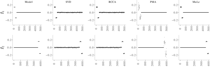
Figure 1: Comparing performance of different sCCA approaches in recovering the sparsity pattern and estimating active elements of the canonical directions. The Model or “true” canonical directions are plotted in the leftmost plot.

Under the same setting, but varying level of noise $\sigma$, we compute the cosine of the angle between the estimated, $\hat{\bm{z}}_{i}$, and true, $\bm{z}_{i}$, canonical directions, $cos(\theta_{i})=|\langle\bm{z}_{i},\hat{\bm{z}}_{i}\rangle|$ for $i=1,2$ via the methods utilized in Figure 1. We plotted the results in Figure 2 for both canonical directions; according to which, MuLe outperforms other methods, especially the alternating method of Witten and Tibshirani (2009), throughout the range of noise amplitude. PMA uniquely shows a lot of volatility in its solution. The built-in parameter tuning also misspecified the correct sparsity parameters, but providing correct hyperparameters manually also did not help much. Actually, our test shows that a simple thresholding algorithm like SVDthr outperforms PMA both in terms of support recovery and direction estimation.

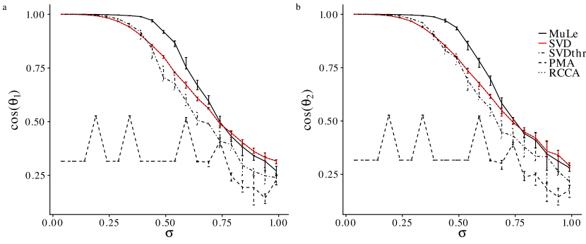
Figure 2: The cosine of the angle between the estimated and true canonical directions, $cos(\theta_{i})=|\langle\hat{\bm{z}}_{i},\bm{z}_{i}\rangle|$ computed for both datasets.

But perhaps the most important piece of information one looks for in high-dimensional multi-view studies is the interpretability of the estimated canonical directions. Therefore, ultimately the decisive criteria in choosing the best approach is determined by how well they uncover the “true” underlying sparsity pattern or simply put, how accurately a model performs variable selection. To this end, variable selection accuracy of each method is plotted against the noise amplitude in Fig. 3 as the fraction of the support of $\bm{z}_{i}$, $i\in\{1,2\}$ discovered, here denoted as $\eta_{i}$, vs. the noise amplitude, $\sigma$. As before MuLe performs significantly better than other methods throughout the noise amplitude range.

7.2 Solution Stability on Data Without Underlying Sparse CCA Model

In the following simulations, $\bm{X}_{1}$ and $\bm{X}_{2}$ are generated by sampling from $\mathcal{N}(\bm{0}_{p_{i}},\bm{I}_{p_{i}}),i\in\{1,2\}$. The main purpose of this section is to demonstrate the stability of the solution paths while comparing the quality of the solutions of different algorithms as a function of the cardinality of the canonical loadings. The motivation behind this simulation is that the solution of a stable algorithm must grow more similar to the non-sparse CCA solution. Therefore, while setting the sparsity parameter equal to zero for one canonical direction, for an array of sparsity parameters we compute the correlation of the estimated direction with the corresponding direction from the CCA solution, as well as the estimated canonical correlation for the same setting.

The results of the aforementioned simulation is presented in Figure 3. According to our results MuLe is consistently more correlated with the CCA solution and for $(\gamma_{1},\gamma_{2})=(0,0)$, it solves the CCA problem whereas PMA by far does not show the same solution stability. Were columns of $\bm{X}_{i}$ more correlated, PMA and SVDThr would have resulted in even worse solutions.

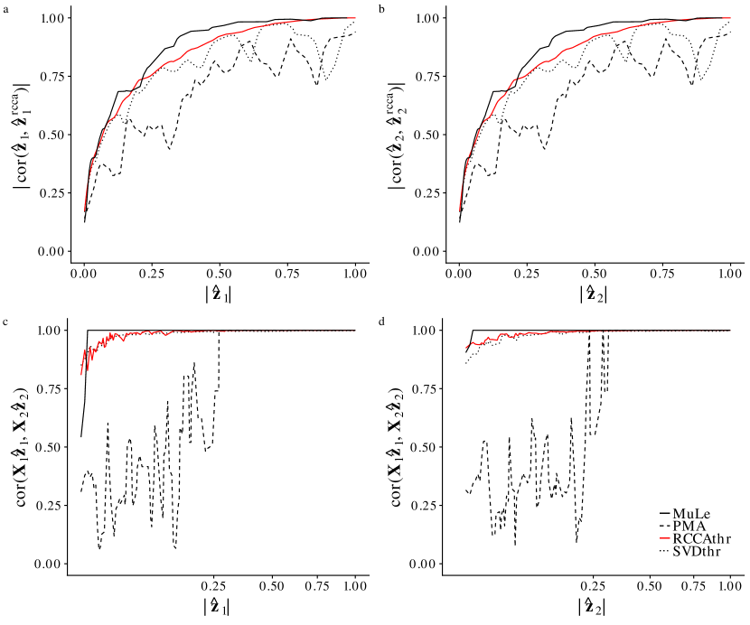
Figure 3: The correlation between the estimated sparse canonical direction and the direction obtained from CCA. (a,b) and the estimated canonical correlation as a function of the cardinality of the estimated direction. (c,d)

In the next section we utilize MuLe to discover correlation structures in a genomic setting.

8 Fruitfly Pesticide Exposure Multi-Omics

One of the drivers for the development of our method was the rise of multi-omics analysis in functional genomics, pharmacology, toxicology, and a host of related disciplines. Briefly, multiple “omic” modalities, such as transcriptomics, metabolomics, metagenomics, and many other possibilities, are executed on matched (or otherwise related) samples. An increasingly common use in toxicology is the use of transcriptomics and metabolomics to identify, in a single experiment, the genetic and metabolic networks that drive resilience or susceptibility to exposure to a compound[Campos and Colbourne (2018)]. We analyzed recently generated transcriptomics, metabolomics, and 16S DNA metabarcoding data generated on isogenic Drosophila (described in Brown et al. 2019, in preparation). In this experiment, fruit flies are separated into treatment and control groups, where treated animals are exposed to the herbicide Atrazine, one of the most common pollutants in US drinking water. Dosage was calculated as 10 times the maximum allowable concentration in US drinking water – a level frequently achieved in surface waters (streams and rivers) and rural wells.

Data was collected after 72 hours, and little to no lethality was observed. Specifically, male and female exposed flies were collected, whereafter mRNA, small molecular metabolites, and 16S rDNA (via fecal collection and PCR amplification of the V3/V4 region) was collected. RNA-seq and 16S libraries were sequenced on an Illumina MiSeq, and polar and non-polar metabolites were assayed by direct injection tandem mass spectrometry on a Thermo Fisher Orbitrap Q Exactive. Here, we compare 16S, rDNA and metabolites using MuLe, to identify small molecules associated with microbial communities in the fly gut microbiome.

This is an intriguing question, as understanding how herbicide exposure remodels the gut microbiome, and, in turn, how this remodeling alters the metabolic landscape to which the host is ultimately exposed is a foundational challenge in toxicology. All dietary co-lateral exposures are ”filtered through the lens” of the gut microbiome – compounds that are rapidly metabolized by either the host system or the gut are experienced, effectively, at lower concentrations; the microbiome plays an important role in toxicodynamics.

We utilized the multi-view sparse CCA module of MuLe to find three-way associations in our study. Hyper-parameter was performed using our permutation test of Algorithm 7 modified to lean towards more sparse models. Our analysis, see Figures 4 and 5, revealed three principle axes of variation. The first groups host genes for primary and secondary metabolism, cell proliferation, and reproduction along with host metabolites related to antioxidant response. Intriguingly, all metabolites in this axis of variation derive from the linoleic acid pathway, part of the anti-oxidant defense system, which is known to be engaged in response to Atrazine exposure [Sengupta et al. (2015)]. Similarly, Glutathione S transferase D1 (GstD1), a host gene that varies along this axis, is a secondary metabolic enzyme that leverages glutathione to neutralize reactive oxygen species (eletrophilic substrates). Linoleic acid metabolites are known to strongly induce glutathione synthesis [Arab et al. (2006)]. The primary metabolism gene, Cyp6w1 is strongly up-regulated in response to atrazine [Sieber and Thummel (2009)], and here we see it is also tightly correlated with the anti-oxidant defense system. We see broad inclusion of cell proliferation genes (CG6770, CG16817, betaTub56D,) and genes involved in reproduction (the Chorion proteins, major structural components of the eggshell chorion, Cp15, Cp16, Cp18, Cp19, Cp38, and Vitelline membrane 26Aa (Vm26Aa)), and it is well known that flies undergo systematic repression of the reproductive system during exposure to environmental stress [Brown et al. (2014)]. Whether this reproductive signal is directly associated with linoleic acid metabolism and glutathione production is an intriguing question for future study.

The second principle axis of variation groups a dominant microbial clade (Lactobacillales) along with a collection of host metabolites, and one gene of unknown function. The host metabolites fall principally on the phosphorylcholine metabolic pathway, which is known to be induced in a sex-specific fashion in response to atrazine in mammals, but, as far as we know, not previously reported in arthopods [Holásková et al. (2019)] – which may be useful, as it expands the domain of mammalian adverse outcome pathways that can be modeled in Drosophila.

The third and final principle axis includes two host genes – a cytochrome P450 (Cyp4g1) known to be involved in atrazine detoxification [Sieber and Thummel (2009)], and a peptidase of unknown function (CG12374) – a minority microbial clade (Rhodospirillales, [Chandler et al. (2011)]), and another collection of linoleic acid pathway metabolites, along with 1-Oleoylglycerophosphoinositol, a host metabolite derived from oleic acid. While the ostensible lack of known microbial metabolites is somewhat disappointing, it may also be that these were simply not assigned chemical IDs during the metabolite identification – a common challenge with untargeted chemistry.

Figure 4: CCA biplot of transcriptomic, microbiomic, and metabolomic datasets in Drosophila Atrazine exposure experiment.

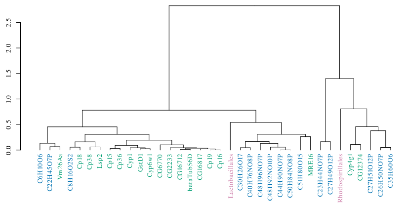
Figure 5: Hierarchical clustering of the first two pairs of canonical directions.

In order to verify that the primary effect captured in our canonical directions are co-variations associated with the treatment effect, and not that of sex, exposure length etc., we also projected our samples on to the plane of the first two canonical covariates, see Figure 6. We then color-coded the samples according to the treatment vector. We observed that our estimated canonical covariates clearly separate our samples according to the treatment effect.

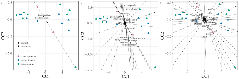
Figure 6: Interpolative plots of microbiomics(a), metabolomics(b), and transcriptomics(c) views. Any given sample is interpolated by either the complete parallelogram or the vector sum method explained in Appendix D.2

Overall, we see many of the genes and metabolites involved in response to Atrazine identified in the support of the first and second canonical covariates. The fact that many members of individual pathways were returned together is comforting – genes and metabolites in the same or related pathways should co-vary, and they appear to through the lens of our analysis. The novelty and discovery of the sCCA method lies in identifying potential interactions between these pathways – and the current analysis has yielded a number of hypotheses for follow-up studies, including the coupling of germ cell proliferation repression to Linoleic acid metabolism. The identification of genes of unknown function is also interesting – we posit that MRE16 along the second principle axis of variation encodes at least one small functional peptide (e.g. a peptidase or an immunopeptide), and this too will be the subject of future study.

9 Conclusion

A two-stage approach to sparse CCA problem was introduced, where in the first stage we computed the sparsity patterns of the canonical directions via a fast, convergent concave minimization program. Then we used these sparsity patterns to shrink our problem to a CCA problem of two drastically smaller matrices, where regular CCA methods may be used. We then extended our methods to multi-view settings, i.e. Multi-View Sparse CCA, where we have more than two views and also to scenarios where our objective is to generate targeted hypotheses about associations corresponding to a specific experimental design, i.e. Directed Sparse CCA. We benchmarked our algorithm and also compared it to several other popular algorithms. Our simulations clearly demonstrated superior solution stability and convergence properties, as well as higher accuracy both in terms of the correlation of the estimated canonical covariates and also in terms of its ability to recover the underlying sparsity patterns of the canonical directions. We also introduced MuLe which is the package implementing our algorithms. We then applied our method to a multi-omic study aiming to understand mechanisms of adaptations of Drosophila Melanoger (Fruitfly) to environmental pesticides, here Atrazine. Our analysis clearly indicated that the estimated canonical directions, while sparse and interpretable, captures co-variations due to the treatment effect, and also the selected sets of covariates are known, according to the peer-reviewed literature, to be associated with adaptation mechanisms of fruitfly to environmental pesticides and stressors.

A Proofs

A.1 Proof of Proposition 15

Let’s assume without loss of generality that $p_{1}\leq p_{2}$. In this case we can start MuLe to find the sparsity pattern of $\bm{z}_{2}\in\mathbb{R}^{p_{2}}$ first, shrink $\bm{X}_{2}$ to $\bm{X}_{2red}\in\mathbb{R}^{n\times n_{2}^{{}^{\prime}}}$ where $n_{2}^{{}^{\prime}}\sim n$, then repeat the same for $\bm{z}_{1}\in\mathbb{R}^{p_{1}}$, shrink $\bm{X}_{1}$ to $\bm{X}_{1red}\in\mathbb{R}^{n\times n_{1}^{{}^{\prime}}}$ where $n_{1}^{{}^{\prime}}\sim n$, and finally compute the first canonical covariates using the shrunken $\bm{X}_{1red}^{T}\bm{X}_{2red}\in\mathbb{R}^{n_{1}^{{}^{\prime}}\times n_{2}^{{}^{\prime}}}$.

According to the setup of algorithm 2, each iteration to find $\bm{\tau}_{2}$ is $O(2p_{1}p_{2}+4p_{1}+p_{1})$, using $\bm{\tau}_{2}$ and shrinking $\bm{X}_{2}$, each iteration for finding $\bm{\tau}_{1}$ is $O(2p_{1}n_{2}^{{}^{\prime}}+4p_{1}+n_{2}^{{}^{\prime}})$ which makes the time complexity of both $O(2p_{1}p_{2}+4p_{1}+p_{1}+2p_{1}n_{2}^{{}^{\prime}}+4p_{1}+n_{2}^{{}^{\prime}})$. With pSVDht, the time complexity of both passes together is $O(4p_{1}p_{2}+2(p_{1}+p_{2}))$. Assuming $p_{2}/p_{1}=k=o(1)$ and $n\sim n_{2}^{{}^{\prime}}$, if

$$n<\frac{2kp_{1}^{2}-2(k+1)p_{1}-p_{1}}{2p_{1}+1}$$

The time complexity of MuLe is less than pSVDht. If $p_{1}>>1$,

$$\frac{2kp_{1}^{2}-2(k+1)p_{1}-p_{1}}{2p_{1}+1}\approx\frac{2kp_{1}^{2}-2(k+1)p_{1}-p_{1}}{2p_{1}}=kp_{1}-(k+0.5)>p_{1}$$

So as long as $n<min\{p_{1},p_{2}\}$, our claim stands.

A.2 Proof of Proposition 16

Here, just to provide more clarity, Algorithm 3 of Witten and Tibshirani (2009) is provided as a representative for the bigger family of sSVD algorithms.

Data: Sample Covariance Matrices $\Sigma_{12}=X_{1}^{T}X_{2}$

   $l_{1}$-penalty parameters $c_{1},c_{2}$

Result: $z_{1}\in\mathbb{R}^{p_{1}}$, $z_{2}\in\mathbb{R}^{p_{2}}$, and $d=z_{1}^{T}\Sigma_{12}z_{2}$

1 Initialize $z_{2}$ to have $l2-norm$ 1;

2 while  convergence criterion is not met  do

3       $z_{1}\leftarrow\frac{S(\Sigma_{12}z_{2},\Delta_{1})}{\|S(\Sigma_{12}z_{2},\Delta_{1})\|_{2}}$ where $\Delta_{1}=0$ if this results in $\|z_{1}\|_{1}\leq c_{1}$; otherwise, $\Delta_{1}$ is chosen to be a positive constant such that $\|z_{1}\|_{1}=c$

4       $z_{2}\leftarrow\frac{S(\Sigma_{12}^{T}z_{1},\Delta_{2})}{\|S(\Sigma_{12}^{T}z_{1},\Delta_{2})\|_{2}}$ where $\Delta_{2}=0$ if this results in $\|z_{2}\|_{1}\leq c_{2}$; otherwise, $\Delta_{2}$ is chosen to be a positive constant such that $\|z_{2}\|_{1}=c$

5       $d\leftarrow z_{1}^{T}\Sigma_{12}z_{2}$

Algorithm 8 $PMD(L_{1},L_{1})$ as proposed in Witten and Tibshirani (2009)

There is no need for a detailed time complexity analysis, as it is evident that although MuLe has order two polynomial time complexity, refer to Appendix A.1, the optimization problems in stages 3 and 4 of PMD, i.e. finding $\Delta_{1}$ and $\Delta_{2}$ that results in $\|z_{1}\|_{1}=c_{1}$ and $\|z_{2}\|_{1}=c_{2}$, are of exponential time complexity $O(2^{p}_{1})$ and $O(2^{p}_{2})$. They propose a binary search algorithm for this problem which has less time complexity but doesn’t have guaranteed convergence, neither heuristically nor theoretically. In the implementation of the algorithm in the PMA package, the maximum number of iterations is set to a very small number, replacing which with a convergence criteria did not prove to be successful.

B Complementary Methods and Algorithms

B.1 Multi-Factor MuLe

Data: Sample Covariance Matrix $\bm{C}_{12}$

   Regularization parameter vectors $\bm{\gamma}_{i}\in\mathbb{R}^{m},i\in\{1,2\}$

   Initial value vectors $\bm{z}_{i}\in\mathcal{S}^{p_{i}},i\in\{1,2\}$

Result: $\bm{Z}_{i}\in\mathbb{R}^{p_{i}\times m},i\in\{1,2\}$

1 Let $\bm{C}_{12}^{(0)}\leftarrow\bm{C}_{12}$

2 for $i=1,\ldots,m$ do

3      

4      $(\bm{z}_{1}^{*(i)},\bm{Z}_{2}^{*(i)}\leftarrow sCCA_{MuLe}(\bm{C}_{12}^{(i-1)},\gamma_{1i},\gamma_{2i})$

5      

6      $\bm{C}_{12}^{(i)}=\bm{C}_{12}-\sum_{k=1}^{i}(\bm{z}_{1}^{(k)*\top}\bm{C}_{12}^{(k-1)}\bm{z}_{2}^{(k)*})\bm{z}_{1}^{(k)*}\bm{z}_{2}^{(k)*\top}$

7      $(\bm{Z}_{1}[,i],\bm{Z}_{2}[,i])\leftarrow(\bm{z}_{1}^{*(i)},\bm{z}_{2}^{*(i)})$

Algorithm 9 Multi-Factor MuLe

B.2 Multi-View CCA as Generalized Eigenvalue Problem

Here, we frame the CCA problem applied to multiple datasets, $\bm{X}_{i}$, $i=1,\ldots,m$, analyzed in Kettenring (1971) as the following Generalized Eigenvalue Problem,

$$\begin{bmatrix}\bm{0}&\bm{C}_{12}^{\prime}&\dots&\bm{C}_{1m}^{\prime}&\\ \bm{C}_{21}^{\prime}&\bm{0}&&\vdots\\ \vdots&&\ddots&\bm{C}_{(m-1)m}^{\prime}\\ \bm{C}_{m1}^{\prime}&&\bm{C}_{m(m-1)}^{\prime}&\bm{0}\end{bmatrix}\begin{bmatrix}\bm{z}_{1}^{\prime}\\ \bm{z}_{2}^{\prime}\\ \vdots\\ \bm{z}_{m}^{\prime}\end{bmatrix}=\lambda\begin{bmatrix}\bm{C}_{11}^{\prime}&\bm{0}&\dots&\bm{0}\\ \bm{0}&\bm{C}_{22}^{\prime}&&\vdots\\ \vdots&&\ddots&\bm{0}\\ \bm{0}&\dots&\bm{0}&\bm{C}_{mm}^{\prime}\end{bmatrix}\begin{bmatrix}\bm{z}_{1}^{\prime}\\ \bm{z}_{2}^{\prime}\\ \vdots\\ \bm{z}_{m}^{\prime}\end{bmatrix}$$ (70)

where $\bm{C}_{ij}^{\prime}$ is the shrunken $\bm{C}_{ij}$, or the sample covariance matrix of the active entries of $\bm{z}_{i}$ and $\bm{z}_{j}$, denoted here as $\bm{z}_{i}^{\prime}$ and $\bm{z}_{j}^{\prime}$. Equation 70 can be solved using a wide variety of solvers. We used the geigen function which is implemented in an r-package of the same name, which uses the routines implemented in LAPACK. Given that $m$ is usually less than 10, and $\bm{z}_{i}^{\prime}=O(n)$, where $n$ is not very large given we’re assuming high-dimensional settings, problem 70 does not involve very large matrices.

B.3 Multi-View SVD via Power Iteration

We proposed a Multi-View CCA in Appendix B.2 which served as the second stage of out two-stage sCCA approach which was to estimate active elements of the canonical directions. Although 70 is of reasonable size, it still requires inversions which might be deemed as a disadvantage. Although it’s very trivial to use ridge regularization to alleviate this issue, here we propose an algorithm which uses power iterations to perform multi-View SVD.

Data: Shrunk Sample Covariance Matrices $\bm{C}_{rs}^{\prime},\quad 1\leq r<s\leq m$

   Initial values $\bm{z}_{r}^{\prime}\in\mathcal{S}^{|\bm{\tau}_{r}|},\quad 1\leq r\leq m$

Result: $\bm{z}_{r}^{\prime}$, $r=1,\ldots,m$, estimated active elements of $\bm{z}_{r}$

1 initialization;

2 for $r=m,\ldots,1$ do

3       while  convergence criterion is not met  do

4            

5            $\bm{z}_{r}^{\prime}\leftarrow\sum_{s=1}^{r}\bm{C}_{sr}(\bm{C}_{sr}^{\top}\bm{z}_{r}^{\prime})+\sum_{s=r+1}^{m}\bm{C}_{rs}^{\prime}\bm{z}_{s}^{\prime}$

6             $\bm{z}_{r}\leftarrow\frac{\bm{z}_{r}}{\|\bm{z}_{r}\|_{2}}$

7      

Algorithm 10 MuLe algorithm for optimizing Program 39

B.4 Two-Stage Directed CCA

Though simple and obvious, we include this approach in this appendix for the sake of clarity and completeness. Here are the steps for this algorithm.

1. Perform variable selection via univariate regression or classification of $\bm{y}$ on each $\bm{X}_{i}$ resulting in a set of variables, $Q_{i}$, which are highly associated with the accessory variable.

2. Subset every datasets such that only the columns selected in the previous steps are kept, resulting in $\bm{X}_{i}^{\prime}\in\mathbb{R}^{n\times|Q_{i}|}$.

3. Perform sCCA between the datasets using any of the algorithms implemented in MuLe.

C Further Experimmentations

C.1 Rank-One Sparse Multi-View CCA Model

To assess the validity of the formulation presented in Program 32 and accuracy of our solution and algorithm presented in Section 6.4, for the cases involving more than two, the rank-one model introduced in Section 7.1 is extended to three datasets by generating $\mathbf{X}_{3}$ as follows,

$$\begin{split}\mathbf{X}_{3}=(\mathbf{z}_{3}+\epsilon_{3})u^{T},&\quad\mathbf{z}_{3}\in\mathcal{R}^{600},\quad\epsilon_{3}\sim\mathcal{N}(0,0.1^{2}),\forall i=1,\ldots,600,\\ \mathbf{z}_{1}&=\bigg{[}\underbrace{1,\ldots,1}_{25}\quad\underbrace{0,\ldots,0}_{550}\quad\underbrace{-1,\ldots,-1}_{25}\bigg{]}\end{split}$$ (71)

where $\mathbf{u}_{i}\sim\mathcal{N}(0,1),\forall i=1,\ldots,50$.

The coefficient estimates are presented in Figure 7. Here, we also included the RGCCA package. Although their conventional sCCA algorithm results were identical to PMA, their generalization to more than two datasets resulted in different and better results. Hence, its inclusion in this simulation. We used each package’s own built-in hyper-parameter tuning procedure to find the best parameters. As evident from the results, MuLe identifies the underlying model quite accurately, but RGCCA although does a good job on parameter estimation, it does a very poor job on recovering the sparsity patterns of the canonical directions. PMA misses both critera quite significantly.

In the next section we utilize MuLe to discover correlation structures in a genomic setting.

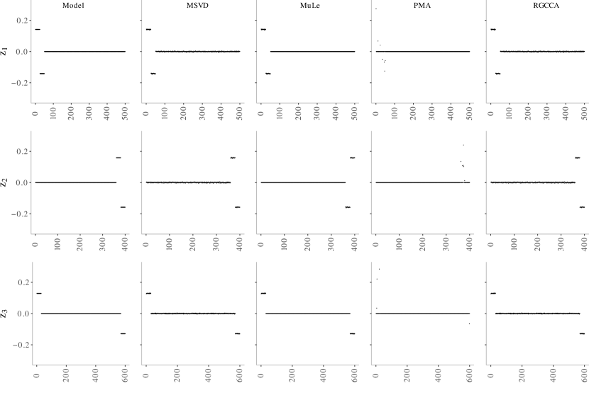
Figure 7: Comparing performance of some of the most common multi-view sCCA approaches to that of MuLe in recovering the sparsity pattern and estimating active elements of the canonical directions. The Model or “true” canonical directions are plotted in the leftmost plot.

D Visualization Methods

In a general subspace learning problem involving datasets, we’re seeking to replace each dataset with three low-dimensional pieces of information, a rule for projecting the original covariates to the learned subspace for the respective subspace, a low-dimensional projection of samples from the original sample-space to the learned sub-space, and a measure of similarity or alignment between the learned subspace. In our linear sCCA context, we replace the dataset $\bm{X}_{i}$ with $\bm{Z}_{i}$ whose rows contain the correlation of the covariate $\bm{x}_{i}$ with the canonical covariates, $\bm{CC}_{i}$ the projection of samples onto the canonical directions and the canonical correlations $\bm{\rho}_{i}^{(j)}\in\mathbb{R}^{m}$ containing the correlation between the $j$-th canonical covariate of the $i$-th dataset and the $j$-th canonical covariates obtained from other datasets. Now we explain the procedures used to create the figures in Section 8 which facilitate the interpretation of sCCA results. Inspired by the methods proposed in Alves and Oliveira (2003), we adapt their CCA biplot and interpolative plot to our sCCA settings. In the following brief tutorial, we focus on the first two canonical covariates, thereby keeping only the first two columns of $\bm{Z}_{i}$ and $\bm{CC}_{i}$, denoted by $\bm{Z}_{i}^{(2)}$ and $\bm{CC}_{i}^{(2)}$, and only $\bm{\rho}_{i}^{(j)}$ for $j\in\{1,2\}$ and $i=\{1,\ldots,m\}$.

D.1 CCA Biplot

In order to create the CCA biplot, e.g. Figure 4, we simply plot the first two columns of $\bm{Z}_{i}^{(2)}$ in the same plot. A key complementary piece of information facilitating interpretation are the first two canonical correlations. Utilizing at this plot, we can form hypotheses about how and to what extend groups of variables from different datasets are associated with each other. The length of the vectors indicate the variable’s share in each canonical direction, while the angle between them indicate their degree of association.

D.2 CCA Interpolative Plots

Another informative visualization we exploit to interpret sCCA results are Interpolative CCA Plots, e.g. Figure 6. In order to create such figure for each dataset, we first plot $\bm{CC}_{i}$ from all datasets in the same plot, which by itself provides enlightening insights into how strongly the samples from different datasets align with each other. Next we need to add lines corresponding to the variables from the respective dataset. In order to make interpolation easier and the plots more clear, we first choose a set of marker points $\bm{\mu}_{ij}$ corresponding to the $j$-th variable from the $i$-th dataset, consisting of values within the range of observed values of the variable $\bm{x}_{ij}$, i.e. $\mu_{ijk}\in[min(\bm{x}_{ij}),max(\bm{x}_{ij})]$. We project these points using the following projection $\bm{\mu}_{ij}\bm{e}_{ij}\bm{V}_{i}^{(2)}$, where $\bm{e}_{ij}$ is a vector whose elements except the $j$-th is zeroed out. Finally, we pass a line through the projected points. Marking the values of each variable corresponding to a sample as a vector along each variable we can find the interpolated position of the said sample. This is a powerful tool as we can find how accurately we can interpolate a samples position using the values of a different dataset. This is specially important in cases where sample matching from different datasets are not exact and samples are matched based on some other metadata, e.g. gender, age etc.

Supplemental Materials: Sparse Canonical Correlation Analysis via Concave Minimization

1 MuLe Package

An R-implementation of our package MuLe, named MuLe-R, along with the scripts used to perform the simulations and create the visualizations, and the data used in Section 8 is available online at https://github.com/osolari/MuleR.

References

- Akaho (2001) S. Akaho. A kernel method for canonical correlation analysis. In Proceedings of the International Meeting of the Psychometric Society, 2001.
- Alam et al. (2008) Md. A. Alam, M. Nasser, and K. Fukumizu. Sensitivity analysis in robust and kernel canonical correlation analysis. 11th International Conference on Computer and Information Technology, 0:399–404, 2008.
- Alves and Oliveira (2003) M Rui Alves and M Beatriz Oliveira. Interpolative biplots applied to principal component analysis and canonical correlation analysis. Journal of Chemometrics: A Journal of the Chemometrics Society, 17(11):594–602, 2003.
- Andrew et al. (2013) G. Andrew, R. Arora, J. Bilmes, and K. Livescu. Deep canonical correlation analysis. International Conference on Machine Learning, pages 1247–1255, 2013.
- Arab et al. (2006) Khelifa Arab, Adrien Rossary, Laurent Soulere, and Jean-Paul Steghens. Conjugated linoleic acid, unlike other unsaturated fatty acids, strongly induces glutathione synthesis without any lipoperoxidation. British Journal of Nutrition, 96(5):811–819, 2006.
- Bach and Jordan (2002) F.R. Bach and M.I. Jordan. Kernel independent component analysis. Journal of machine learning research, pages 1–48, 2002.
- Bach and Jordan (2005) F.R. Bach and M.I. Jordan. A probabilistic interpretation of canonical correlation analysis. Technical Report, 2005.
- Baur and Bozdag (2015) B. Baur and S. Bozdag. A canonical correlation analysis-based dynamic bayesian network prior to infer gene regulatory networks from multiple types of biological data. Journal of Computational Biology, 22(4):289–299, 2015.
- Benson (1995) Harold P Benson. Concave minimization: theory, applications and algorithms. In Handbook of global optimization, pages 43–148. Springer, 1995.
- Blaschko et al. (2008) M.B. Blaschko, C.H. Lampert, and A. Gretton. Semi-supervised laplacian regularization of kernel canonical correlation analysis. Joint European Conference on Machine Learning and Knowledge Discovery in Databases, 0:133–145, 2008.
- Brown et al. (2014) James B Brown, Nathan Boley, Robert Eisman, Gemma E May, Marcus H Stoiber, Michael O Duff, Ben W Booth, Jiayu Wen, Soo Park, Ana Maria Suzuki, et al. Diversity and dynamics of the drosophila transcriptome. Nature, 512(7515):393, 2014.
- Cai (2013) J. Cai. The distance between feature subspaces of kernel canonical correlation analysis. Mathematical and Computer Modelling, 3:970–975, 2013.
- Campos and Colbourne (2018) Bruno Campos and John K Colbourne. How omics technologies can enhance chemical safety regulation: perspectives from academia, government, and industry: The perspectives column is a regular series designed to discuss and evaluate potentially competing viewpoints and research findings on current environmental issues. Environmental toxicology and chemistry, 37(5):1252, 2018.
- Cao et al. (2015) L. Cao, Z. Ju, J. Li, R. Jian, and C. Jiang. Sequence detection analysis based on canonical correlation for steady-state visual evoked potential brain computer interfaces. Journal of neuroscience methods, 0(253):10–17, 2015.
- Chandler et al. (2011) James Angus Chandler, Jenna Morgan Lang, Srijak Bhatnagar, Jonathan A Eisen, and Artyom Kopp. Bacterial communities of diverse drosophila species: ecological context of a host–microbe model system. PLoS genetics, 7(9):e1002272, 2011.
- Cichonska et al. (2016) A. Cichonska, J. Rousu, P. Marttinen, A.J. Kangas, P. Soininen, T. Lehtimäki, O.T. Raitakari, M.R. Järvelin, V. Salomaa, M Ala-Korpela, and others. metacca: Summary statistics-based multivariate meta-analysis of genome-wide association studies using canonical correlation analysis. Bioinformatics, 32:1981–9, 2016.
- Dunham and Kravetz (1975) R.B. Dunham and D.J. Kravetz. Canonical correlation analysis in a predictive system. The Journal of Experimental Education, 43(4):35–42, 1975.
- d’Aspremont et al. (2008) Alexandre d’Aspremont, Francis Bach, and Laurent El Ghaoui. Optimal solutions for sparse principal component analysis. Journal of Machine Learning Research, 9(Jul):1269–1294, 2008.
- Ewerbring and Luk (1989) L.M. Ewerbring and F.T. Luk. Canonical correlations and generalized svd: applications and new algorithms. In 32nd Annual Technical Symposium, International Society for Optics and Photonics, page 206–222, 1989.
- Fang et al. (2016) J. Fang, D. Lin, Z. Xu S.C. Schulz, V.D. Calhoun, , and Y.P. Wang. Joint sparse canonical correlation analysis for detecting differential imaging genetics modules. Bioinformatics, 32(22):3480–3488, 2016.
- Friman et al. (2001) O. Friman, J. Cedefamn, P. Lundberg, M. Borga, and H. Knutsson. Detection of neural activity in functional mri using canonical correlation analysis. Magnetic Resonance in Medicine, 45:323–330, 2001.
- Gestel et al. (2001) T. Van Gestel, J.A.K. Suykens, J. De Brabanter, B. De Moor, and J. Vandewalle. Kernel canonical correlation analysis and least squares support vector machines. International Conference on Artificial Neural Networks., pages 384–389, 2001.
- Hardoon et al. (2004) David R Hardoon, Sandor Szedmak, and John Shawe-Taylor. Canonical correlation analysis: An overview with application to learning methods. Neural computation, 16(12):2639–2664, 2004.
- Hardoon and Shawe-Taylor (2009) D.R. Hardoon and J. Shawe-Taylor. Convergence analysis of kernel canonical correlation analysis: theory and practice. Machine learning., 1:23–38, 2009.
- Hardoon and Shawe-Taylor (2011) D.R. Hardoon and J. Shawe-Taylor. Sparse canonical correlation analysis. Machine Learning, 3:331–353, 2011.
- Healy (1957) M.J.R. Healy. A rotation method for computing canonical correlations. Math. Comp., 58:83–86, 1957.
- Heij and Roorda (1991) C. Heij and B. Roorda. A modified canonical correlation approach to approximate state space modeling. Proceedings of the 30th IEEE Conference on Decision and Control, pages 1343–1348, 1991.
- Holásková et al. (2019) Ida Holásková, Meenal Elliott, Kathleen Brundage, Ewa Lukomska, Rosana Schafer, and John B Barnett. Long-term immunotoxic effects of oral prenatal and neonatal atrazine exposure. Toxicological Sciences, 168(2):497–507, 2019.
- Hopkins (1969) C.E. Hopkins. Statistical analysis by canonical correlation: a computer application. Health services research, 4(4):304, 1969.
- Hotelling (1935) H. Hotelling. The most predictable criterion. Journal of Educational Psychology, 26:139–142, 1935.
- Hyman et al. (2002) E. Hyman, P. Kauraniemi, S. Hautaniemi, M. Wolf, S. Mousses, E. Rozen-blum, M. Ringner, G. Sauter, O. Monni, A. Elkahloun, O.-P. Kallioniemi, and A. Kallioniemi. Impact of dna amplication on gene expression patterns in breast cancer. Cancer Research, 0(62):6240–6245, 2002.
- Journée et al. (2010) M. Journée, Y. Nesterov, P. Richtrárik, and R. Sepulchre. Generalized power method for sparse principal component analysis. Journal of Machine Learning Research, 11:517–553, 2010.
- Kettenring (1971) Jon R Kettenring. Canonical analysis of several sets of variables. Biometrika, 58(3):433–451, 1971.
- Klami et al. (2012) A. Klami, S. Virtanen, and S. Kaski. Bayesian exponential family projections for coupled data sources. arXiv:1203.3489, 2012.
- Lai and Fyfe (1999) P.L. Lai and C. Fyfe. A neural implementation of canonical correlation analysis. Neural Networks, 10:1391–1397, 1999.
- Lai and Fyfe (2000) P.L. Lai and C. Fyfe. Kernel and nonlinear canonical correlation analysis. International Journal of Neural Systems, 10:365–377, 2000.
- Larson et al. (2014) N.B. Larson, G.D. Jenkins, M.C. Larson, R.A. Vierkant, T.A. Sellers, C.M. Phelan, J.M. Schildkraut, R. Sutphen, P.P.D. Pharoah, S. A. Gayther, et al. Kernel canonical correlation analysis for assessing gene–gene interactions and application to ovarian cancer. European Journal of Human Genetics, 1:126–131, 2014.
- Lindsey et al. (1985) H. Lindsey, J.T. Webster, , and S. Halper. Canonical correlation as a discriminant tool in a periodontal problem. Biometrical journal, 3(27):257–264, 1985.
- Mangasarian (1996) OL Mangasarian. Machine learning via polyhedral concave minimization. In Applied Mathematics and Parallel Computing, pages 175–188. Springer, 1996.
- Melzer et al. (2001) T. Melzer, M. Reiter, and H. Bischof. Nonlinear feature extraction using generalized canonical correlation analysis. International Conference on Artificial Neural Networks., 0:353–360, 2001.
- Mercer (1909) James Mercer. Xvi. functions of positive and negative type, and their connection the theory of integral equations. Philosophical transactions of the royal society of London. Series A, containing papers of a mathematical or physical character, 209(441-458):415–446, 1909.
- Monmonier and Finn (1973) M.S. Monmonier and F.E. Finn. Improving the interpretation of geographical canonical correlation models. The Professional Geographer, 25:140–142, 1973.
- Morley et al. (2004) M. Morley, C. Molony, T. Weber, J. Devlin, K. Ewens, R. Spielman, and V. Cheung. Genetic analysis of genome-wide variation in human gene expression. Nature, 0(430):743–747, 2004.
- Nakanishi et al. (2015) M. Nakanishi, Y. Wang, Y.T Wang, and T.P. Jung. A comparison study of canonical correlation analysis based methods for detecting steady-state visual evoked potentials. PloS one, 10(10):10–17, 2015.
- Ogura et al. (2013) T. Ogura, Y. Fujikoshi, and T. Sugiyama. A variable selection criterion for two sets of principal component scores in principal canonical correlation analysis. Communications in Statistics-Theory and Methods, 42(12):2118–2135, 2013.
- Orsini et al. (2018) Luisa Orsini, James B Brown, Omid Shams Solari, Dong Li, Shan He, Ram Podicheti, Marcus H Stoiber, Katina I Spanier, Donald Gilbert, Mieke Jansen, et al. Early transcriptional response pathways in daphnia magna are coordinated in networks of crustacean-specific genes. Molecular ecology, 27(4):886–897, 2018.
- Ouarda et al. (2001) T. B. M. J. Ouarda, C. Girard, G. S. Cavadias, and B. Bobée. Regional flood frequency estimation with canonical correlation analysis. Journal of Hydrology, 254:157–173, December 2001. doi: 10.1016/S0022-1694(01)00488-7.
- Parkhomenko et al. (2007) E. Parkhomenko, D. Tritchler, and J. Beyene. Genome-wide sparse canonical correlation of gene expression with genotypes. BMC Proceedings, 1:s119, 2007.
- Parkhomenko et al. (2009) E. Parkhomenko, D. Tritchler, and J. Beyene. Sparse canonical correlation analysis with application to genomic data integration. Statistical Applications in Genetics and Molecular Biology, 8:1–34, 2009.
- Pollack et al. (2002) J. Pollack, T. Sorlie, C. Perou, C. Rees, S. Jerey, P. Lonning, R. Tibshi-rani, D. Botstein, A. Borresen-Dale, and P. Brown. Microarray analysis reveals a major direct role of dna copy number alteration in the transcriptional program of human breast tumors. Proceedings of the National Academy of Sciences, 0(99):12963–12968, 2002.
- Rousu et al. (2013) J. Rousu, D.D. Agranoff, O. Sodeinde, J. Shawe-Taylor, and D. Fernandez-Reyes. Biomarker discovery by sparse canonical correlation analysis of complex clinical phenotypes of tuberculosis and malaria. PLoS Comput Biol, 9(4), 2013.
- Sarkar and Chakraborty (2015) B.K. Sarkar and C. Chakraborty. Dna pattern recognition using canonical correlation algorithm. Journal of biosciences, 40(4):709–719, 2015.
- Schell and Gardner (1995) S.V. Schell and W.A. Gardner. Programmable canonical correlation analysis: A flexible framework for blind adaptive spatial filtering. IEEE transactions on signal processing, 43(12):2898–2908, 1995.
- Sengupta et al. (2015) Namrata Sengupta, Elizabeth J Litoff, and William S Baldwin. The hr96 activator, atrazine, reduces sensitivity of d. magna to triclosan and dha. Chemosphere, 128:299–306, 2015.
- Seoane et al. (2014) J.A. Seoane, C. Campbell, I.N.M. Day, J.P. Casas, and T.R. Gaunt. Canonical correlation analysis for genebased pleiotropy discovery. PLoS Comput Biol, 10(10), 2014.
- Shen et al. (2013) X-B Shen, Q-S Sun, and Y-H Yuan. Orthogonal canonical correlation analysis and its application in feature fusion. 16th International Conference on Information Fusion, pages 151–157, 2013.
- Sieber and Thummel (2009) Matthew H Sieber and Carl S Thummel. The dhr96 nuclear receptor controls triacylglycerol homeostasis in drosophila. Cell metabolism, 10(6):481–490, 2009.
- Simonson et al. (1983) D. Simonson, J. Stowe, and C. Watson. A canonical correlation analysis of commercial bank asset/liability structures. Journal of Financial and Quantitative Analysis, 10:125–140, 1983.
- Snijders et al. (2017) Antoine M Snijders, Sasha A Langley, Young-Mo Kim, Colin J Brislawn, Cecilia Noecker, Erika M Zink, Sarah J Fansler, Cameron P Casey, Darla R Miller, Yurong Huang, et al. Influence of early life exposure, host genetics and diet on the mouse gut microbiome and metabolome. Nature microbiology, 2(2):16221, 2017.
- Tu et al. (1989) X.M. Tu, D.S. Burdick, D.W. Millican, and L.B. McGown. Canonical correlation technique for rank estimation of excitation-emission matrices. Analytical Chemistry, 19(61):2219–2224, 1989.
- Vinod (1976) H.D. Vinod. Canonical ridge and econometrics of joint production. Journal of Econometrics, 4:147–166, 1976.
- Waaijenborg et al. (2008) S. Waaijenborg, P. Verselewel de Witt Hamer, and A. Zwinderman. Quantifying the association between gene expressions and dna-markers by penalized canonical correlation analysis. Statistical Applications in Genetics and Molecular Biology, 7, 2008.
- Wang et al. (2013) G.C. Wang, N. Lin, and B. Zhang. Dimension reduction in functional regression using mixed data canonical correlation analysis. Stat Interface, 6:187–196, 2013.
- Wang et al. (2016) Weiran Wang, Xinchen Yan, Honglak Lee, and Karen Livescu. Deep variational canonical correlation analysis. arXiv preprint arXiv:1610.03454, 2016.
- Waugh (1942) F.V. Waugh. Regressions between sets of variables. Econometrica, Journal of the Econometric Society, page 290–310, 1942.
- Wiesel et al. (2008) Ami Wiesel, Mark Kliger, and Alfred O Hero III. A greedy approach to sparse canonical correlation analysis. arXiv preprint arXiv:0801.2748, 2008.