Single spin resonance driven by electric modulation of the $g$ factor anisotropy

Abstract

We address the problem of electronic and nuclear spin resonance of an individual atom on a surface driven by a scanning tunnelling microscope. Several mechanisms have been proposed so far, some of them based on the modulation of exchange and crystal field associated to a piezoelectric displacement of the adatom driven by the RF tip electric field. Here we consider a new mechanism, where the piezoelectric displacement modulates the $g$ factor anisotropy, leading both to electronic and nuclear spin flip transitions. We discuss thoroughly the cases of Ti-H ($S=1/2$) and Fe $(S=2)$ on MgO, relevant for recent experiments. We model the system using two approaches. First, an analytical model that includes crystal field, spin orbit coupling and hyperfine interactions. Second, we carry out density functional based calculations. We find that the modulation of the anisotropy of the $g$ tensor due to the piezoelectric displacement of the atom is an additional mechanism for STM based single spin resonance, that would be effective in $S=1/2$ adatoms with large spin orbit coupling. In the case of Ti-H on MgO, we predict a modulation spin resonance frequency driven by the DC electric field of the tip.

I Introduction

The quest of single spin electron paramagnetic resonance (EPR) driven with a scanning tunneling microscope (STM) has been pursued for many years Manassen et al. (1989); Balatsky et al. (2012). The first report of STM-ESR of individual adatoms on a surface of MgO(100)/Ag Baumann et al. (2015a) has been followed by several dramatic breakthroughs in the study of spin physics of individual magnetic atomsNatterer et al. (2017); Choi et al. (2017); Yang et al. (2017); Willke et al. (2018a, b); Bae et al. (2018); Yang et al. (2018, 2019); Willke et al. (2019a, b). This technique permits to carry out absolute measurements of the magnetic moment of individual atomsNatterer et al. (2017); Choi et al. (2017). The spectral resolution achieved so far, down to a few MHz, has made it possible to resolve the hyperfine structure of Fe, Ti and Cu atomsWillke et al. (2018b); Yang et al. (2018). In the case of Cu adatoms, the electrical driving of nuclear spin-flip transitions that preserve the electronic spin has been demonstrated as wellYang et al. (2018). Thus, STM-EPR permits to drive the electronic and nuclear spins of individual atoms on surfaces, as well as artificially created structures, such as dimersYang et al. (2017); Bae et al. (2018). Importantly, the STM-ESR technique is being now implemented in several different laboratories, at higher temperaturesNatterer et al. (2019) and higher driving frequencies Seifert et al. (2019).

An important question in the STM-EPR contextBaumann et al. (2015a); Natterer et al. (2017); Choi et al. (2017); Yang et al. (2017); Willke et al. (2018a, b); Bae et al. (2018); Yang et al. (2018, 2019); Willke et al. (2019a), and also for experiments reporting electric control of individual nuclear spin in single molecule transport Thiele et al. (2014); Godfrin et al. (2017), is the understanding of how electric fields couple both to electronic and nuclear spin degrees of freedom. This question has also been addressed in other systems. The idea of electric dipole spin resonance was proposed back in 1960 by RashbaRashba (1960). Electrical control of spin qubits has been reported in semiconductor nanostructures, based both on modulation of the $g$ factorKato et al. (2003) and on inhomogeneous magnetic fieldsTokura et al. (2006); Pioro-Ladriere et al. (2008). Electric fields have been used to drive spin resonance of itinerant electrons in InSbBell (1962) and localized magnetic dopants in ZnOGeorge et al. (2013).

In the seminal paper of Baumann et alBaumann et al. (2015a), where the first STM-EPR experiment was carried out with Fe atoms on an MgO surface, a mechanism was proposed to account for the coupling of the STM voltage to the electronic spin, that depended on the specific details of the microscopic Hamiltonian of that system. The mechanism is based on the assumption that the $RF$ field induces a vertical piezoelectric displacement of the adatom, $\delta z\propto eV_{RF}$, that in turns modifies the crystal field Hamiltonian of the $d$ orbitals of Fe. This modulation, together with spin-orbit coupling and a strong in-plane Zeeman field, would lead to spin transitions between the two lowest energy states of the $S=2,S_{z}=\pm 2$ of Fe, a non-Kramers doublet integer spin system Hoffman (1994).

Other mechanisms have been proposed to account for the driving of the surface spin by the tip bias voltageBalatsky et al. (2012); Berggren and Fransson (2016); Lado et al. (2017); Shakirov et al. (2019); Gálvez et al. (2019). For instance, in Ref. [Lado et al., 2017] we proposed a mechanism based on the modulation of the exchange interaction between the magnetic tip and the magnetic adatom, that originates also from the piezoelectric distortion of the adatom.

Here we propose another complementary mechanism, that can coexist with the others, based on the electric modulation of the $g$ tensor associated to the piezoelectric distortion of the adatom. As in the case of the crystal fieldBaumann et al. (2015a) and exchangeLado et al. (2017); Yang et al. (2019) mechanisms, we also assume that the magnetic adatom undergoes a piezoelectric displacement. In turn, this modulation changes the crystal field parameters that control the anisotropy of the electronic spin interactions, that leads to an anisotropic $g$ factor and to a renormalization of the hyperfine coupling. As we show below, these modulations lead both to electronic and nuclear spin flip transitions.

The rest of this paper is organized as follows. In section II we present a general argument to show that an anisotropic time dependent modulation of the $g$ tensor of a $S=1/2$ system leads to electronic spin transitions. In section III we briefly present a single particle Hamiltonian for a $d^{1}$ adatom with $C_{4}$ symmetry, valid for Ti-H adatom on the oxygen site of MgO(001). In section IV we present our description of the Ti-H adatom on MgO based on Density functional theory (DFT) calculations and how this connects with the crystal field Hamiltonian presented in the previous section.

In section V we derive analytical expressions for the $g$ tensor anisotopy of Ti-H on MgO, based on the model of section III. The $g$ tensor obtained depends on the Ti spin-orbit coupling and the crystal field parameters, that can be obtained from DFT. In section VI we discuss how the $g$ factor can be modulated for Ti-H on MgO by application of an electric field between tip and surface and we compute the associated Rabi energy. In section VII we briefly present the analogous piezoelectric modulation for Fe on MgO. In section VIII we discuss how the contact hyperfine interaction become anisotropic due to the $g$ factor anisotropy and how the $g$ factor modulation could induce nuclear spin flip transitions. In section IX we discuss the role of both the $g$ tensor anisotropy of the adatom and the magnetic anisotropy of the tip in the efficiency of the exchange modulation Lado et al. (2017) mechanism. In section X we show that the DC component of the tip-surface electric field induces a shift of the transition energy of the adatom due to the modification of the $g$ tensor. Finally, in section XI we present some limitations of our models and we list our main conclusions. The appendices describe technical steps of some results used in the main text.

II Spin transitions driven by anisotropic modulation of the $g$ tensor

For a free electron in vacuum, the interaction with a magnetic field is perfectly isotropic, in the sense that the energy splitting is the same regardless of the direction of the magnetic field $\vec{B}$. This results leads to the isotropic Zeeman interaction, $g\mu_{B}\vec{S}\cdot\vec{B}$ . In contrast, for a general class of systems, the interplay between the spin orbit coupling $\vec{\ell}\cdot\vec{S}$, the orbital coupling to the magnetic field $\vec{\ell}\cdot\vec{B}$, and the crystal field splitting leads to an anisotropic Zeeman interaction. For instance, in the case of $S=1/2$ adatoms, such as Ti-H Yang et al. (2017); Willke et al. (2018b); Bae et al. (2018); Yang et al. (2018, 2019) and CuYang et al. (2018) on a $001$ MgO surface, the interplay between the spin orbit coupling and the crystal field splitting leads to an anisotropic Zeeman interaction with different off-plane ($z$) and in-plane $xy$:

$${\cal H}_{Z}=g_{x}\mu_{B}B_{x}S_{x}+g_{z}\mu_{B}B_{z}S_{z}=\mu_{B}\vec{b}_{0}\cdot\vec{S}$$ (1)

where $\vec{b}_{0}=(g_{x}B_{x},0,g_{z}B_{z})$.

As we show below, the tip $ac$ electric field modulates the $g_{x}$ and $g_{z}$ coefficients, resulting in a time dependent perturbation:

$${\cal V}(t)=(\delta g_{x}\mu_{B}B_{x}S_{x}+\delta g_{z}\mu_{B}B_{z}S_{z})\cos(2\pi ft)$$ (2)

This equation can be written down as

$${\cal V}(t)=\cos(2\pi ft)\mu_{B}\vec{b}_{1}\cdot\vec{S}$$ (3)

where $\vec{b}_{1}=(\delta g_{x}B_{x},0,\delta g_{z}B_{z})$. This perturbation can induce spin transitions between the two eigenstates of ${\cal H}_{0}$ if $\vec{b}_{0}$ and $\vec{b}_{1}$ are non-collinear, $|\vec{b}_{1}\times\vec{b}_{0}|\neq 0$. This yields

$$\frac{\delta g_{z}}{g_{z}}\neq\frac{\delta g_{x}}{g_{x}}$$ (4)

Thus, the perturbation (2) induces spin transitions if the relative modulations of the $g$ factor are different. If we express the perturbation Hamiltonian in the basis of eigenstates of ${\cal H}_{Z}|\pm\rangle=\pm\frac{\Delta_{Z}}{2}|\pm\rangle$:

$${\cal V}(t)=\Omega_{g}\cos(2\pi ft)\left(|+\rangle\langle-|+|-\rangle\langle+|\right)$$ (5)

where the Rabi coupling $\Omega_{g}$ is given by particularly simple equation, derived in appendix A:

$$\Omega_{g}=\frac{\Delta_{Z}}{4}\sin 2\theta\left(\frac{\delta g_{z}}{g_{z}}-\frac{\delta g_{x}}{g_{x}}\right)$$ (6)

where $\Delta_{z}\equiv\mu_{B}|\vec{b}_{0}|$ is the Zeeman splitting, $\theta$ is the polar coordinate of the $\vec{b}_{0}$ defined in Eq. (1) (see also Eq. (55), Eq. (65) and Eq.(66)). From Eq. (6) we immediately infer that the Rabi coupling created by the modulation of the $g$ factor scales linearly with the magnitude of the magnetic field, and has a very strong dependence on its orientation relative to the normal of the surface.

III A model Hamiltonan for T${\rm i}$-H on M${\rm g}$O

We now consider a toy model that describes a single electron occupying a $d$ shell with a crystal field splitting with $C_{4}$ symmetry for rotations in the $xy$ plane around the $z$ axis. This permits to obtain closed analytical expressions for the $g$ tensor in terms of the crystal field parameters and the spin orbit coupling. In addition, our DFT calculations, discussed below, show that the model provides a fairly good description of hydrogenated Ti adatoms on the oxygen site of an MgO surface, relevant for STM-EPR experimentsYang et al. (2017); Willke et al. (2018b); Yang et al. (2018); Bae et al. (2018); Yang et al. (2019).

Ti²⁺ on MgO has 2 electrons in the $d$ shell, and our DFT calculations show it has $S=1$, in contrast with the experimental results Yang et al. (2017); Willke et al. (2018b); Bae et al. (2018); Yang et al. (2018, 2019). It has been proposed that the reason why Ti/MgO has $S=1/2$ is because it chemisorbs an hydrogen atomYang et al. (2017). Our DFT calculations back up this assumptionYang et al. (2017). They show that hydrogen sits on top of Ti, almost co-linear with the Oxygen-Ti line that goes perpendicular to the surface. In that geometry, the $s$ orbital of $H$ hybridizes both with $d_{z^{2}}$ and $s$ orbital of Ti and forms a molecular bonding-anti-bonding pair that hosts 2 electrons. This leaves only a single electron in the $d$ shell, that occupies the $x^{2}-y^{2}$ orbital, so that the Ti-H system effectively has $S=1/2$. We use the following Hamiltonian for the outermost electron of a single $S=1/2$ electron in a $d$ shell, that includes crystal field terms, spin orbit coupling and Zeeman interaction:

$${\cal H}_{0}=-|D|\ell_{z}^{2}+F\left((\ell^{(+)})^{4}+(\ell^{(-)})^{4}\right)+$$

$$+\lambda\vec{S}\cdot\vec{\ell}+\mu_{B}\vec{B}\cdot\left(g\vec{S}+\vec{\ell}\right)$$ (7)

Here, $\ell$ is the single particle angular momentum operator for the $d$ electrons and $\vec{S}$ are the spin 1/2 matrices. Notice that Baumann et al.Baumann et al. (2015a) used a mathematically similar expression for a multi-electronic Hamiltonian multiplet with $L=S=2$, valid for Fe on MgO. The crystal field terms account for the electrostatic interactions of the first neighbour charged ions of the Ti adatom (see Fig. 1). Mg atoms are positively charged ions that reduce the energy of the $xy$ and $x^{2}-y^{2}$ orbitals compared to the $xz$, $yz$ and z² orbitals. Oxygen atom is negatively charged and it increase the energy of the $z^{2}$ orbital. The $D$ term accounts for these effects. In addition, the $F$ term accounts for the $C_{4}$ symmetry of the surface, and discriminates between the $xy$ and $x^{2}-y^{2}$ orbitals, as one of them points towards the positively charged Mg ions, reducing the energy of that orbital, whereas the other points towards the oxygen atoms. The lowest energy orbital should be the $x^{2}-y^{2}$ (if we take the oxygen atoms in the $(10)$ and $(01)$ directions).

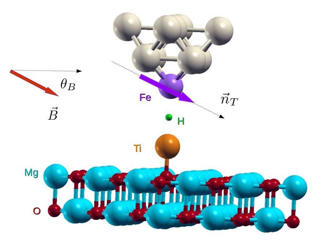
Figure 1: Scheme of the STM-ESR experimental set-up Baumann et al. (2015a); Natterer et al. (2017); Choi et al. (2017); Yang et al. (2017); Willke et al. (2018a, b); Bae et al. (2018); Yang et al. (2018, 2019); Willke et al. (2019a) with the atomic structure of Ti-H on the oxygen site of MgO. $\vec{B}$ is the external magnetic field applied during the experiment (with an angle $\theta_{B}$ measured with respect to the surface) and $\vec{n}_{T}$ shows the direction of the magnetic moment of the tip. Red balls represent O atoms, blue balls Mg atoms, violet ball is for Fe atom, green ball for H atom and the orange one is for Ti atom.

IV Density Functional Calculations for Hydrogenated T${\rm i}$

In this section we focus on the electronic properties of individual Hydrogenated Ti ad-atoms at MgO on-top-of-oxygen, as described with density functional theory (DFT) calculations. With this aim, we have employed Quantum EspressoGiannozzi et al. (2009), using projected augmented wave pseudopotentials, PBE exchange correlation functional and 50-70 Ry of plane wave energy cut-off as described elsewhere Giannozzi et al. (2009); Perdew et al. (1998); Blöchl (1994). We performed calculations in a structure formed by a bilayer of MgO, as shown in Fig. 1, consisting in 36 O atoms (red balls) and 36 Mg Atoms (blue balls) together with the hydrogenated Ti (orange ball) with one H (green ball). In order to check some results we also performed a few number of calculations using a bigger supercell with 64 O atoms, 64 Mg Atoms and the hydrogenated Ti. The main distortions created by the ad-atom in the MgO bilayer are: (i) an upward displacement of the closest oxygen(s) to ad-atoms and (ii) a distortion downwards of the Mg atoms located below the Ti-bonded oxygen atoms. Our DFT calculations found that a hydrogenated Ti atom shows $S=1/2$ Yang et al. (2017); Willke et al. (2018b). The spin density of hydrogenated TiO (with the Ti and H atoms located collinear along the $z$ axis) is consistent with a filling of the $d_{x^{2}-y^{2}}$ orbital, since we are assuming that the Mg atoms first neighbour of oxygen are in the $x$ and $y$ axis.

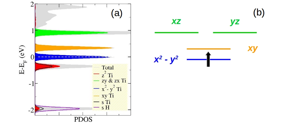
Figure 2: (a) DFT calculations for the Spin-unpolarized Density of States projected over $d-$ and $s-$ orbitals of Ti and the $s-$orbital of Hydrogen. The grey shadow shows the total density of states. (b) Energy level cartoon.

Fig 2(a) shows the projected density of states over $d-$orbitals for the hydrogenated Ti at MgO on-top-of-oxygen, computed with no spin polarization. DFT yields $x^{2}-y^{2}$ and a hybrid orbital $z^{2}-s$ as the lowest energy orbitals, within the $d$ manifold. The $z^{2}$ of the Ti $d$ shell is strongly hybridized with the hydrogen $1s$ orbital. As a result, the $z^{2}$ and the $s$ are split in energy and, altogether host 2 electrons. The $xy$ orbital comes next in energy, and is empty. The orbital doublet $xz$ and $yz$ lies higher up in energy. Calculations show that $x^{2}-y^{2}$ hosts exactly one electron. It is apparent that the Hamiltonian model Eq. (7) with $\ell_{z}=\pm 1,\pm 2$ describes the $4$ orbitals $x^{2}-y^{2}$, $xy$, $xz$ and $yz$.

IV.1 Connection between DFT and model Hamiltonian

We now explain how to obtain a rough estimate of $D$ and $F$ parameters that enter in the crystal field Hamiltonian (7). The method amounts to fit the energy difference of the peaks in the density of states obtained from a spin-unpolarized DFT calculation to those obtained from Eq. (7):

$$E_{x^{2}-y^{2}}-E_{xy} = 48F$$ (8)

$$2E_{xz}-E_{x^{2}-y^{2}}-E_{xy} = 6|D|$$ (9)

Using these equations, from inspection of the density of states we infer the values $D\simeq-255$ meV and $F\simeq 7.50$ meV. This crude approximation is enough for the scope of this work.

We can also obtain an estimates for the modulation of the crystal field parameters, $D$ and $F$, as the length of the Ti-O bond is changed from its equilibrium position. The calculation is carried out moving Ti atom and relaxing the four closest neighbor Mg atoms, the O atom below and the H atom, keeping all the others fixed. The results of the parameters $D$ and $F$, obtained with this procedure allows us to obtain the following relation between $D$, $F$ and the strain:

$$\frac{dF}{dz} = -6\frac{\rm meV}{\AA}$$ (10)

$$\frac{dD}{dz} = +188\frac{\rm meV}{\AA}$$ (11)

These values are used later on to estimate how the piezoelectric displacement of the Ti-O bond modulates the crystal field values $F$ and $D$, that in turn modulate the $g$ tensor.

IV.2 Calculation of the $g$ tensor from DFT

We have calculated the $g$ tensor components from our DFT calculations using Gauge Including Projector Augmented Waves (GIPAW). GIPAW is a DFT based method to calculate magnetic resonance properties Pickard and Mauri (2002), where spin-orbit coupling is implemented in a perturbative way. Our calculations for the structure in equilibrium $\delta z=0$, give us a diagonal $g$-tensor with components $g_{x}=g_{y}=1.974$ and $g_{z}=1.881$. As we discuss now, the model Hamiltonian Eq. (7) provides physical insight on the origin of the anisotropy, and very good agreement with the values obtained from DFT.

V Calculation of the $g$ tensor from the model

We now use the model Hamitlonian Eq. (7) to compute the $g$ tensor. We do this at two levels of approximation. First, we obtain analytical approximate expressions from the model Hamiltonian. Second, we obtain the $g$ tensor from the exact numerical solution of the model. Both, the analytical and numerical approach permit to relate the $g$ tensor components with the crystal field parameters $D$ and $F$ and the spin orbit coupling $\lambda$. On account of the $C_{4}$ symmetry of the Hamiltonian, the $g$ tensor is diagonal, and has $g_{x}=g_{y}$. Therefore, we only need to compute $g_{z}$ and $g_{x}$.

V.1 Calculation of $g_{z}$

We first consider the response of the electron in the $x^{2}-y^{2}$ state to a magnetic field in the $z$ direction. For that matter we need to consider the space of 4 states with $\ell_{z}=\pm 2$ and $S_{z}=\pm 1/2$. Within this subspace, spin orbit coupling only acts through the $S_{z}\ell_{z}$ term. Therefore, $S_{z}$ is conserved, and the Hamiltonian for each $S_{z}$ is given by:

$${\cal H}_{S_{z}}(B_{z})=\left(\begin{array}[]{cc}-\lambda\ell_{z}S_{z}+\Delta_{-}(B_{z})&24F\\ 24F&\lambda\ell_{z}S_{z}+\Delta_{+}(B_{z})\end{array}\right)$$ (14)

where $\Delta_{\pm}(B_{z})=\mu_{B}B_{z}(gS_{z}\pm\ell_{z})$ with $\ell_{z}=2$. Hamiltonian Eq. (14) can be written as:

$${\cal H}(S_{z})=g\mu_{B}B_{z}S_{z}+\vec{h}(S_{z})\cdot\vec{\sigma}$$ (15)

where

$$\vec{h}(S_{z})=\left(24F,0,-\ell_{z}(\mu_{B}B_{z}+S_{z}\lambda)\right)$$ (16)

We thus have $\epsilon_{2}(S_{z},\pm)=-4|D|+E^{(\pm)}(S_{z})$, where:

$$E^{(\pm)}(S_{z})=g\mu_{B}B_{z}S_{z}\pm\sqrt{(24F)^{2}+\ell_{z}^{2}(\mu_{B}B_{z}+S_{z}\lambda)^{2}}$$

We now Taylor expand the ground state of the $E^{-}$ states around $B_{z}=0$:

$$E^{(-)}(S_{z})=-\sqrt{(24F)^{2}+\lambda^{2}}+g\mu_{B}S_{z}B_{z}+\delta g_{z}S_{z}\mu_{B}B_{z}$$

where

$$g_{z}=g+\delta g_{z}=2-\frac{4\lambda}{\sqrt{(24F)^{2}+\lambda^{2}}}$$ (17)

Interestingly, there are no higher order corrections to $\delta g_{z}$, coming from mixing with the $\ell_{z}=\pm 1$ manifold. This is confirmed by the comparison of eq. (17) with the results obtained from exact diagonalization of the complete model (7). As a result, we can use equation (17) for obtain the ratio $\frac{F}{\lambda}=1.4$ that gives $g_{z}$ in agreement with the DFT result $g_{z}=1.881$ The dependence of $g_{z}$ on $\lambda$, $F$ and $D$ is shown in Fig. (3). Note that, as shown in Fig. (4), $g_{z}$ does not depend on $D$ and we can use $F/\lambda=1.4$ to ensure that $g_{z}=1.881$.

V.2 Calculation of $g_{x}$

We now obtain an analytical expression for $g_{x}$ for the $x^{2}-y^{2}$ ground state manifold of Hamiltonian Eq. (14). For that matter, we represent the operator $\mu_{B}B_{x}(gS_{x}+\ell_{x})$ in the basis of eigenstates of ${\cal H}(\sigma)$:

$$|\psi_{-}(\uparrow)\rangle = \cos\frac{\alpha}{2}|-2,\uparrow\rangle-\sin\frac{\alpha}{2}|+2,\uparrow\rangle$$

$$|\psi_{-}(\downarrow)\rangle = \cos\frac{\alpha}{2}|+2,\downarrow\rangle-\sin\frac{\alpha}{2}|-2,\downarrow\rangle$$

where the angle $\alpha$ is defined as

$$\vec{h}(S_{z})=|\vec{h}(S_{z})|\left(\sin\alpha(S_{z}),0,\cos\alpha(S_{z})\right)$$ (18)

and $\vec{h}$ is defined in Eq. (16). In this subspace the matrix elements of $\ell_{x}$ are zero and the only non zero matrix element of $S_{x}$ reads:

$$\langle\psi^{-}(\uparrow)|S_{x}|\psi^{(-)}(\downarrow)\rangle=-\frac{1}{2}\sin\alpha$$ (19)

For $B_{z}=0$, we have

$$\sin\alpha=\frac{24F}{\sqrt{(24F)^{2}+\lambda^{2}}}\;\;\;\cos\alpha=\frac{-|2S_{z}|\lambda}{\sqrt{(24F)^{2}+\lambda^{2}}}$$ (20)

Thus, the eigenvalues of the Hamiltonian are:

$$\epsilon_{2}(B_{x})=-3|D|-\sqrt{(24F)^{2}+\lambda^{2}}\pm\frac{g}{2}\mu_{B}B_{x}\sin\alpha$$ (21)

We thus have:

$$g_{x}^{(1)}=g\sin\alpha=g\frac{24F}{\sqrt{(24F)^{2}+\lambda^{2}}}$$ (22)

We now consider the contributions to $g_{x}$ that arise from the virtual transitions to the $\ell=\pm 1$ levels. These are driven by the combined action of the $\mu_{B}\ell_{x}B_{x}$ and the flip-flop part of the spin orbit interaction. This additional contribution gives:

$$\delta g_{x}^{(2)}=-\frac{2\lambda}{3|D|+24|F|+|\lambda|}$$ (23)

so that the $g_{x}$ factor is given by:

$$g_{x}=g\frac{24F}{\sqrt{(24F)^{2}+\lambda^{2}}}-\frac{2\lambda}{3|D|+24|F|+|\lambda|}$$ (24)

The anisotropy of the $g$ tensor arises ultimately from the fact that the $\ell_{z}=\pm 2$ states have a strong additional orbital response only when $B$ is applied in the $z$ direction. This extra contribution is quenched by the $F$ crystal field term, that leads to states with equal weight on the two $\ell_{z}=\pm 2$ states, but promoted by the spin orbit coupling. The resulting anisotropy is thus controlled by the competition between $\lambda$ and $F$. In addition, $g_{x}$ has also a contribution that arises from virtual coupling to the $\ell_{z}=\pm 1$ states. For the values of $D,F,\lambda$ adequate to describe Ti-H on MgO, the dominant contribution to the departe of $g_{x}$ from the value $g=2$ arises from the virtual coupling to $\ell=\pm 1$.

So, for $F=0$ we have $g_{x}^{(1)}=0$, because the spin-orbit coupling correlates $S_{z}$ and $\ell_{z}$ so that spin flips entail momentum flips, that are forbidden, and $g_{z}=-2$ because of the dominant orbital contribution. In the opposite limit of $\lambda=0$ we recover $g_{x}=g_{z}=2$. If we repeat the analysis for $g_{y}$ we obtain $g_{x}=g_{y}$, as expected from the C₄ surface’s symmetry.

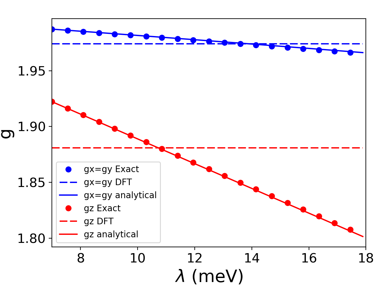
Figure 3: Dependence of $g_{x}$ and $g_{z}$ on spin orbit coupling $\lambda$, for Ti-H on oxygen, obtained in two ways: solution of full model Eq. (7) with $D=$-255 meV and $F=14$ meV (symbols) and using analytical results ignoring $\ell_{z}\neq 2$ manifolds (Eq. (17) and Eq. (24)) (lines). DFT results are shown for reference as dashed lines.

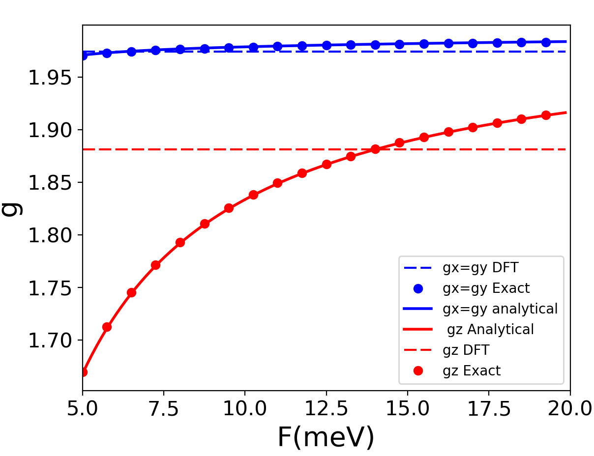
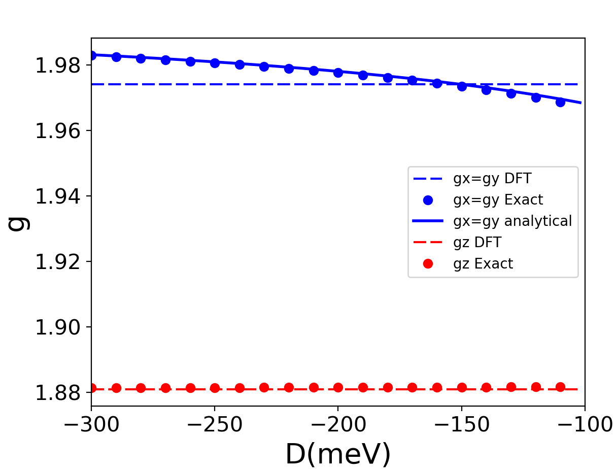
Figure 4: Dependence of $g_{x}$ and $g_{z}$ on crystal field parameters $F$ (top) and $D$ (bottom) for Ti-H on oxygen, obtained from full model Eq. (7) (solid points in both panels), DFT (dashed lies) and analytically (solid lines) (Eq. (17) and Eq. (24)). In both panels we take $\lambda=10$ meV. Top panel: $D=-255$ meV. Bottom panel $F=14$ meV.

In Fig. 3 and Fig. 4 we show the predictions for $g_{x}$ and $g_{z}$, as a function of $\lambda$, $D$ and $F$, obtained using both the analytical formulas Eq. (17), Eq. (24) and the exact solution of the complete Hamiltonian Eq. (7). The DFT results are shown as dashed horizontal lines. In Fig. 3 and Fig. 4 (top) we take $D=-255$ meV, roughly estimated from DFT, using Eq. (9) which gives a single particle spectrum in agreement with the results of DFT. In the bottom panel of Fig. 4 we take $\lambda=10$ meV and $F=14$ meV, also inferred from comparison with DFT. In Fig. 4 we fix $\lambda=10$ meV and $F=1.4\lambda$ so that we obtain values very close to those obtained with DFT. Finally, figure 4 shows that the dependence of $g_{x}$ on $D$ is small, and $g_{z}$ does not depend on $D$.

Summing up , the results of this section show how, for a model with the symmetry adequate for a TiH on top of an oxygen on an $(001)$ MgO surface, the $g$ factor is anisotropic, $g_{z}\neq g_{x}=g_{y}$ and how $g_{z}$ and $g_{x}$ depend on the crystal field parameters $F$, and to a lesser extent, on $D$. Our analytical model is able to give $g_{x}$ and $g_{z}$ in agreement with the values obtained from DFT.

VI Piezoelectric modulation of $g$ for T${\rm i}$-H on M${\rm g}$O

We have shown that a modulation of the $g$ factor anisotropy would induce spin-flip transitions (Eq. (6)), and we have computed how the $g$ factor components depend on the crystal field parameters $F$ and $D$. We now argue that an electric field applied perpendicular to the surface of MgO modulates $F$ and $D$, and thereby the $g$ factor anisotropy, resulting in spin transitions between the two states of the lowest energy Kramers doublet of Eq. (7).

Our DFT calculations show that crystal field parameters $D$ and $F$ are functions of the adatom-oxygen distance, $z$: $D(z)$, $F(z)$ (see Eq. (10) and Eq. (11)). We denote the equilibrium position by $z_{\rm eq}$. The electric field across the gap between the STM and the MgO surface, $E=V_{tip}/d$, where $d$ is the tip-MgO distance, induces a force on the adatom, $F=q_{\rm adatom}V_{\rm tip}/d$ on account of its charge $q_{\rm adatom}$ tBaumann et al. (2015a); Lado et al. (2017); Yang et al. (2019). This force is compensated by a restoring elastic force $F=-k\delta z$. Thus, the adatom equilibrium position is displaced byLado et al. (2017):

$$\delta z(t)=\frac{q_{\rm adatom}V_{\rm tip}(t)}{kd}$$ (25)

This equation is valid for a time dependent $V_{\rm tip}$ as long as its Fourier components are away from the mechanical resonance frequency of the stretching mode, $\sqrt{\frac{k}{M}}$, where $M$ is the mass of the adatom. According to our DFT calculationsLado et al. (2017); Yang et al. (2019), this frequency is up in the THz range, as long as we ignore the contributions coming from the off-plane (flexural) phonons of the MgO. In the following we assume $V_{\rm tip}(t)=V^{0}_{RF}\cos(2\pi ft)$ so that we have

$$\delta z(t)=\frac{q_{\rm adatom}V^{0}_{\rm RF}(t)}{kd}\cos(2\pi ft)\equiv\delta z_{0}\cos(2\pi ft)$$ (26)

From our DFT calculations for Ti-H on MgOYang et al. (2019) we obtain $k=290$ eV nm^-2, so that for RF tip voltages values ranging from $eV^{0}_{RF}=10$ meV to $eV^{0}_{RF}=20$ meV and $d=5\AA$, the piezoelectric displacement amplitude goes from $\delta z_{0}=0.07\,$ pm to $\delta z_{0}=0.14\,$ pm.

The modulation of crystal field parameters $F$ and $D$ with the Ti-O bond length leads to a modulation of the $g$ tensor:

$$\delta g_{a}=\left(\frac{\partial g_{a}}{\partial F}\frac{\partial F}{\partial z}+\frac{\partial g_{a}}{\partial D}\frac{\partial D}{\partial z}\right)\delta z(t)$$ (27)

It must be noted that this equation is also valid in the $DC$ limit.

We now proceed to estimate the magnitude of the Rabi coupling associated to the modulation of the $g$ factor. We do that using two different methods that, as we discuss below, give the same result. The first method consist on using Eq. (6). In the second method we evaluate directly the matrix elements of the crystal field operators, using the same approach used in previous worksBaumann et al. (2015a); Lado et al. (2017).

VI.1 Rabi coupling from the $g$ factor anisotropy

In order to compute the Rabi coupling from eq. (6), we need to compute eq. (27). For that matter, we obtain $\frac{\partial g_{a}}{\partial F}$ and $\frac{\partial g_{a}}{\partial D}$ from our model Hamiltonian, and we use $\frac{\partial F}{\partial z},\frac{\partial D}{\partial z}$ calculated from DFT calculations in Sec. (IV.1).

We are now in position to estimate $\Omega_{g}$, combing Eq. (6), Eq. (10), Eq. (26) and Eq. (27). We now take $V^{0}_{RF}=20$ meV, $d=5\AA$ and $k=290$ev$/{\rm nm}^{2}$ (taken from DFT calculations). This yields a strain of the $Ti-O$ distance of $\delta z_{0}=0.14$pm. In Fig. (5) we plot the magnitude of the Rabi coupling so obtained, as a function of the angle between the magnetic field and the surface, $\theta_{B}$ for $B=1$ Tesla. The first thing to note is that the magnitude of $\Omega_{g}$ is between one and two orders of magnitude smaller than the experimental values reported in our previous workYang et al. (2019). Therefore, other mechanism, most likely exchange modulationLado et al. (2017), has to be involved in the electric field driving of the spin for ESR-STM for Ti-H/MgO.

The magnitude of $\Omega_{g}$ scales linearly both with the applied field $B$ and with the RF electric field $\frac{V_{RF}}{d}$. The optimal angle to maximize $\Omega_{g}$ is close to 45 degrees. In contrast, the exchange mechanism is independent of $B$ and scales exponentiallyYang et al. (2019) with $d$. Whereas the $g$ factor modulation is not dominant for Ti-H on MgO, it could be the dominant factor in heavier adatoms. To show this, in the bottom panel of Fig. 5 we plot $\Omega_{g}$ ramping $\lambda$, keeping all the other parameters the same and taking $\theta_{B}=45$. It is apparent that, for a wide range, $\Omega_{g}$ scales linearly with spin orbit coupling. Expectedly, $\Omega_{g}$ vanishes for $\lambda=0$, as the $g$ factor anisotropy is driven by $\lambda$.

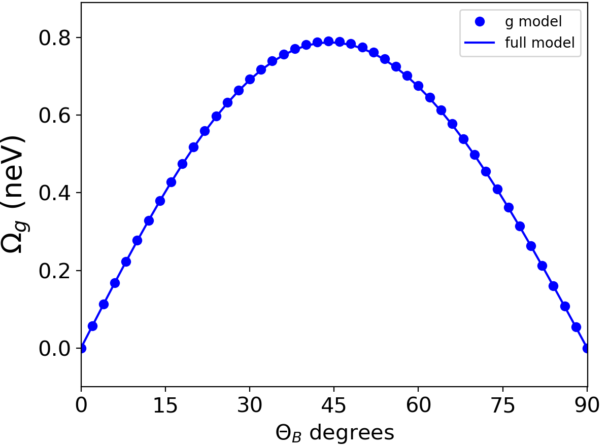
Figure 5: Top: Rabi coupling due to $g$ factor modulation as a function of the angle $\theta_{B}$ between $\vec{B}$ and surface calculated with two methods: Eq. (6) and Eq. (29). $\lambda=10$ meV, $F=1.4\lambda=14$ meV, $D=-255$ meV, $B=1T$, $V_{F}=20$meV, STM-surface distance $d=5\AA$, $k=290$eV$/{\rm nm}^{2}$. Bottom: Dependence of $\Omega_{g}$ on $\lambda$, keeping all the other constants the same and $\theta_{B}=45$ degrees.

VI.2 Rabi coupling from crystal field matrix elements

We now carry out a sanity check. Given that the electronic spin flip transitions described by the effective $S=1/2$ model of Eq. (1) and Eq. (2), arise ultimately from the modulation of the crystal field operators of the parent Hamiltonian of Eq. (7), we have computed the Rabi coupling using the parent model as well. To do so, we first obtain the two lowest eigenstates of Hamiltonian from Eq. (7), ${\cal H}|\pm\rangle=\left(E_{g}\pm\frac{\Delta_{z}}{2}\right)|\pm\rangle$ and we then compute the matrix elements of the perturbation operator:

$${\cal V}(t)=\frac{\partial D}{\partial z}\delta z(t)\ell_{z}^{2}+\frac{\partial F}{\partial z}\delta z(t)\left((\ell^{(+)})^{4}+(\ell^{(-)})^{4}\right)$$ (28)

where the time dependence is described by Eq. (26). We thus define:

$$\Omega_{CF} = \frac{\partial D}{\partial z}\delta z_{0}\langle+|\ell_{z}^{2}|-\rangle+$$ (29)

$$+ \frac{\partial F}{\partial z}\delta z_{0}\langle+|\left((\ell^{(+)})^{4}+(\ell^{(-)})^{4}\right)|-\rangle$$

The results of the calculation of $\Omega_{CF}$ as function of $\theta_{B}$, obtained with the same values of $\lambda$, $D$, $F$, $d$, $V_{RF}$, $k$, and $B$ of the previous subsection, are shown in Fig. 5 and, expectedly, are in full agreement with those obtained using Eq. (6). This agreement validates our analysis.

VII $g$ factor modulation of F${\rm e}$ on M${\rm g}$O

The results of the last paragraph show that it is possible to interpret the modulation spin-driving coming from the modulation of the crystal field parameters (Eq. (29)) in terms of a modulation of the $g$ factor (Eq. 6). In the seminal work of Baumann et al. Baumann et al. (2015b), the modulation of the crystal field (CF) was proposed as the driving mechanism for ESR-STM of Fe/MgO. Here we address the question of whether we can recast the CF mechanism in terms of the $g$ factor modulation, for the case of Fe on MgO as well.

In order to find the answer, that turns out to be negative, we need to model the $g$ factor modulation for Fe on MgO and to compare with the results obtained from the CF modulation. The main difference with the case of Ti-H is that the ground state of Fe on MgO has $S=2$. Therefore, a multi-electronic description is necessaryBaumann et al. (2015a, c); Lado et al. (2017).

We follow our own work Lado et al. (2017) and we model Fe on MgO with a two levels of complexity. First, a microscopic Hamiltonian for 6 electrons in the $d$ orbitals of Fe, in the presence of a crystal field, spin orbit coupling, Coulomb interaction and Zeeman interaction:

$${\cal H}_{\rm Fe}=H_{\rm CF}+H_{\rm SOC}+H_{\rm Z}+V_{ee}$$ (30)

The single particle crystal field Hamiltonian reads:

$${\cal H}_{CF}=D\ell_{z}^{2}+F\left(\ell_{x}^{4}+\ell_{y}^{4}\right)$$ (31)

As explained in the appendix (C), this CF Hamiltonian turns is almost identical to the one we have used in Eq. (7) Ti-H/MgO. As we did in the case of Ti-H/MgO, we can infer $D$ and $F$ from DFT calculations Lado et al. (2017). For $z=z_{eq}$ we obtain, from DFT calculations, $F=-10$ meV and $D=-290$ meV Lado et al. (2017). The spin orbit coupling constant for Fe is $\lambda=35$ meV. Lado et al. (2017)

The many-body Hamiltonian can be solved exactly, by numerical diagonalization in a space made with all the states that accommodate 6 electrons in 5 spin degenerate $d$ orbitals. The lowest energy manifold has 5 states, corresponding to a ground state with $S=2$ and can be described in terms of an effective spin model:

$$H_{\rm eff} = -{\cal D}_{2}S^{2}_{z}+{\cal D}_{4}S^{4}_{z}-{\cal F}(S^{4}_{+}+S^{4}_{-})$$ (32)

$$+ \mu_{B}{\bf B}\cdot g\cdot{\bf S}$$

where the spin operators act on the $S=2$ subspace. The main difference with the $S=1/2$ case is the presence of single ion anisotropy terms. The anisotropy terms ${\cal D}_{2},{\cal D}_{4},{\cal F}$ and the $g$ tensor can be obtained from the diagonalization of Hamiltonian Eq. (30). We obtain ${\cal D}_{2}=4.9$ meV, ${\cal D}_{4}=0.23$ meV and ${\cal F}=11$ $n$eV. With these numbers, the spectrum of the $S=2$ manifold has a ESR active space formed by a doublet of states with $S_{z}=\pm 2$, that we denote as $|0\rangle$ and $|1\rangle$. Yet, this doublet is fundamentally different Hoffman (1994) from the $S=1/2$ Kramers pair, as it has a zero field splitting, given by $\Delta=48{\cal F}=0.5\mu$eV, due to quantum spin tunnelingKlein (1952); Garg (1993); Wernsdorfer and Sessoli (1999); Delgado et al. (2015). Thus, the ESR active doublet for Fe on MgO can not be described in terms of a Zeeman only Hamiltonian. At $B=0$, none of the two lowest energy states has a magnetic momentDelgado et al. (2015). However, application of a modest off-plane field is enough to induce an off-plane magnetic moment in the two lowest energy states, on account of the small value of $\Delta$.

Diagonalizations of the multi-electronic Hamiltonian Eq. (30) at finite magnetic field permit to derive the $g$ tensor. Expectedly for a system with $C_{4}$ symmetry, it is diagonal in the cartesian basis. The values of the $g$ tensor do depend on the single particle crystal field parameters $D$ and most notably on $F$ and $\lambda$. For the values quoted above, we obtain $g_{z}=2.8$ and $g_{x}=g_{y}=2.0$.

Importantly, all the constants in the effective Hamiltonian Eq. (32) do depend strongly on the single particle crystal field parameter $F$, that in turns depends on the piezoelectric displacementLado et al. (2017). Following a similar argument that the one used for $d^{1}$ atoms, we can calculate the Rabi frequency derived from the effective Hamiltonian. We break it down in two types of terms:

$$\Omega_{eff}=\Omega_{ZFS}+\Omega_{g}$$ (33)

The first comes from the modulation of the zero field energy constants, ${\cal D}_{2}$, ${\cal D}_{4}$, and ${\cal F}$ and was absent in the case of $S=1/2$ adatoms . The dominant contributionsLado et al. (2017) arise from the modulation of the $F$ term in the single particle crystal field of Eq. (31):

$$\Omega_{ZFS}=\left(-\frac{\partial{\cal D}_{2}}{\partial F}\langle 0|S^{2}_{z}|1\rangle\right.$$

$$\left.+\frac{\partial{\cal D}_{4}}{\partial F}\langle 0|S^{4}_{z}|1\rangle-\frac{\partial{\cal F}}{\partial F}\langle 0|S^{4}_{+}+S^{4}_{-}|1\rangle\right)\frac{\partial F}{\partial z}$$ (34)

where $\frac{\partial F}{\partial z}=280$meV $/nm$, obtained from DFT in a previous publicationLado et al. (2017). The second class of contribution to the Rabi coupling comes from the $g$ factor modulation, very much like the $S=1/2$ case:

$$\Omega_{g}=\mu_{B}\left(\frac{\partial g_{z}}{\partial F}B_{z}\langle 0|S_{z}|1\rangle+\frac{\partial g_{x}}{\partial F}B_{x}\langle 0|S_{x}|1\rangle\right)\frac{\partial F}{\partial z}$$ (35)

We can assess the relative contribution of the zero field splitting and the $g$ tensor modulations in the following way. We first compute the Rabi coupling using the whole multi-electron HamiltonianLado et al. (2017) and we refer to this as $\Omega_{CI}$. The calculation, done for $B_{z}=0.2$ T , $k=600$ eV$/$nm², $d=0.6$ nm, $V_{RF}=8$ mV, $D=-290$ meV, $F=-10$ meV, $\lambda=35$ meV and $q=2e$ is shown in Fig. (6) as a function of the in-plane field $B_{x}$, together with the different contributions, $\Omega_{ZFS}$ and $\Omega_{g}$, computed using the effective Hamiltonian Eq. (32), Eq. (34) and Eq. (35). It is apparent that the $\Omega_{CI}=\Omega_{ZFS}+\Omega_{g}$, which validates our methods.

Figure 6: . Breakdown of Rabi coupling for Fe on MgO as a function of in plane magnetic field $B_{x}$. The calculation were performed for $B_{z}=0.2$ T , $k=600$ eV$/$nm², $d=0.6$ nm, $V_{RF}=8$ mV, $D=-290$ meV, $F=-10$ meV, $\lambda=35$ meV and $q=2e$

Importantly, our calculations show that the modulation of the $g$ factor is not a dominant contribution to the spin transitions driven by the modulation of the crystal field parameter $F$ due to off-plane piezoelectric distortion of the adatom. In addition, it was found in Ref. Lado et al., 2017 that the exchange modulation mechanism is probably dominant for Fe. Therefore, the $g$ factor modulation plays a marginal role in the case of Fe.

VIII Modulation of the hyperfine interaction

Here we briefly address how the modulation of the $g$ factor anisotropy affects the hyperfine interaction. Recently, electrical control of an individual nuclear spin of $S=1/2$ Cu atom was demonstrated using STM-EPR Yang et al. (2018). For simplicity here we consider the case of Ti-H on MgO, for which hyperfine splittings have been observed experimentally Willke et al. (2018b). We consider a simplified hyperfine model where only the contact interaction term is considered:

$${\cal V}_{\rm HF}=A{\bf I}\cdot{\bf S}$$ (36)

For simplicity, the dipolar and quadruple terms are neglected, although they are known to be relevant for Ti-H on MgOWillke et al. (2018b). We now address how the modulation of the $g$ factor anisotropy affects this Hamiltonian and we find that the effective hyperfine coupling becomes anisotropic.

For that matter, we consider the representation of the isotropic hyperfine operator Eq. (36) in the basis set defined by the tensor product of the lowest energy eigenstates of Hamiltonian Eq. (7), whose wave functions are given by Eq. (V.2), and the eigenstates of the nuclear spin operator $I_{z}$. The resulting Hamiltonian reads:

$${\cal H}_{HF}=A_{||}I_{z}S_{z}+A_{\perp}\left(I_{x}S_{x}+A_{y}I_{y}S_{y}\right)$$ (37)

where

$$A_{||}=A,\;\;A_{\perp}=A\sin\alpha=A\frac{24F}{\sqrt{(24F)^{2}+\lambda^{2}}}$$ (38)

where $F$ and $\lambda$ are the crystal field and spin orbit coupling in Eq. (7). It is apparent that the modification of the hyperfine interaction is connected to the $g$ factor anisotropy.

We now discuss how the modulation of the $g$ factor could lead to nuclear spin-transitions that preserve the electronic spin. We consider the situation where a magnetic field induces an electronic Zeeman splitting so that the eigen-states of the electro-nuclear Hamiltonian can be split in two groups, according to their electronic spinYang et al. (2018). We are interested in transitions between the low energy manifold, so that initial and final state belong to the low energy group, and only the nuclear spin changes in the transition. We thus consider transitions between two eigen-states that differ by single nuclear spin flipYang et al. (2018):

$$|I_{z}\rangle_{-}=\sqrt{1-\epsilon^{2}}|\downarrow\rangle|I_{z}\rangle+\epsilon|\uparrow\rangle|I_{z}-1\rangle$$ (39)

and

$$|I_{z}-1\rangle_{-}=\sqrt{1-\epsilon^{2}}|\downarrow\rangle|I_{z}-1\rangle+\epsilon|\uparrow\rangle|I_{z}-2\rangle$$ (40)

where $\epsilon\propto\frac{A_{\perp}}{g_{z}\mu_{B}B_{z}}<<1$. These states have a dominant $\downarrow$ electronic spin component and a small mixing due to the non-resonant spin-flip hyperfine interaction.

It is apparent that a perturbation that flips the electronic spin can induce transitions between these two states:

$${}_{-}\langle I_{z}-1|S^{-}|I_{z}\rangle_{-}\propto\epsilon\sqrt{1-\epsilon^{2}}\simeq\frac{A_{\perp}}{g_{z}\mu_{B}B_{z}}$$ (41)

showing the electronic driven nuclear spin transition matrix element is proportional to the hyperfine interaction. Thus, the same modulation of the g-tensor that drives electronic spin transitions, when $f$ in the range of the electronic Zeeman transition, can also drive nuclear-spin flip transitions if $f$ is in the range of the hyperfine interaction, as shown experimentally in the case of Cu on MgOYang et al. (2018).

We finally note that the modulation of $F$ will in turn change $A_{\perp}$ providing a time dependent electron-nuclear perturbation,

$$\delta{\cal V}_{HF}=\delta A_{\perp}(t)\left(I_{x}S_{x}+I_{y}S_{y}\right)$$ (42)

where $\delta A_{\perp}=\frac{\partial A_{\perp}}{\partial F}\frac{\partial F}{\partial z}\delta z(t)$. However, this electron-nuclear flip-flop operator can not mix the states (39) and (40). The flip-flip modulation can induce EPR like transitions, between state (39) and

$$|I_{z}-1\rangle_{+}=\sqrt{1-\epsilon^{2}}|\uparrow\rangle|I_{z}-1\rangle+\epsilon|\downarrow\rangle|I_{z}\rangle$$ (43)

This could be a relevant mechanism for ESR-STM in systems with very large hyperfine interaction, such as Bi in silicon George et al. (2010) or perhaps Cu/MgO Yang et al. (2019). Hyperfine driven electric spin dipole resonances have been reported in semiconductor quantum dotsShafiei et al. (2013).

IX Role of anisotropic $g$ factor and the exchange driven mechanism for EPR-STM

Although the main scope of this paper is to propose a new mechanism for the electric field driving of the surface spins in STM-ESR, we briefly comment here on the role that the $g$ factor anisotropy plays on the exchange-modulation mechanism that we proposed in Ref. Lado et al., 2017 and has been experimentally observedYang et al. (2019) for Ti-H adatoms on MgO. We now consider a Hamiltonian for the surface spin that, in addition to the Zeeman term, given by Eq. (1), has also exchange interaction with the tip. The magnetic moment of the tip is described semiclassicallyLado et al. (2017); Yang et al. (2019), so that the Hamiltonian for the surface spin reads:

$${\cal H}_{\rm ex}={\cal H}_{Z}+J(z)\vec{n}_{T}\cdot\vec{S}$$ (44)

where (see Fig. 1)

$$\vec{n}_{T}=\left(\cos(\theta_{B}+\delta),0,\sin(\theta_{B}+\delta)\right)$$ (45)

describes the orientation of the tip moment, $\vec{B}=B_{0}\left(\cos(\theta_{B}),0,\sin(\theta_{B})\right)$ is the external magnetic field forming and angle $\theta_{B}$ with the MgO surface as shown in Fig. 1 and $J(z)$ is the tip-adatom exchange interaction, that depends on the tip-surface distance $z$.

In the appendix A.2 we derive an expression for the Rabi energy associated to the modulation $\delta J$ of the exchange formula:

$$\Omega_{J}={\cal E}_{J}\left(\frac{\Delta g_{x}}{g}-\frac{\Delta g_{z}}{g}\right)\cos\theta_{B}\sin\theta_{B}\cos\delta+$$

$$+{\cal E}_{J}\left(1+\frac{\Delta g_{x}}{g}\cos^{2}\theta_{B}+\frac{\Delta g_{z}}{g}\sin^{2}\theta_{B}\right)\sin\delta$$ (46)

where we write the ansotropic $g$ factor as

$$g_{x}=g+\Delta g_{x}$$

$$g_{z}=g+\Delta g_{z}$$ (47)

where $\Delta g_{x}$ and $\Delta g_{z}$ are the static contributions to the $g$ factor anisotropy and

$${\cal E}_{J}\equiv\frac{\delta J}{2\Delta_{z}^{*}}g\mu_{B}B$$ (48)

and

$$\Delta_{Z}^{*}\equiv\sqrt{(g_{x}\mu_{B}B_{x}+Jn_{x})^{2}+(g_{z}\mu_{B}B_{z}+Jn_{z})^{2}}$$ (49)

Let us consider now two different limits for this complicated formula. We study first the case $\delta=0$, i.e., when the tip magnetic moment is aligned with the external magnetic field. This amounts to assume that the tip magnetic moment has an isotropic $g$ factor. For $\delta=0$ the exchange modulation Rabi splitting reads:

$$\Omega_{J}=\frac{{\cal E}_{J}}{2}\sin 2\theta_{B}\left(\frac{\Delta g_{x}}{g}-\frac{\Delta g_{z}}{g}\right)$$ (50)

Thus, this equation makes it apparent that the $g$ factor anisotropy of the surface spin is essential if the tip spin is aligned with $B$ ($\delta=0$). We note that, in spite of the similar aspect of Eq. (6) and Eq. (50), they describe different mechanisms. In Eq. (6), the transitions are driven by the anisotropic modulation $\delta g$ of the $g$ factor anisotropy. In Eq. (50), the transitions are driven by the modulation of the tip-surface spin $\delta J$, but are enabled by the static $g$ factor anisotropy, given by $\Delta g$.

We now consider the case $\Delta g_{x}=\Delta g_{z}=\Delta g$, i.e., when the surface spin has an isotropic $g$ factor. We obtain:

$$\Omega_{J}={\cal E}_{J}\left(1+\frac{\Delta g}{g}\right)\sin\delta$$ (51)

Thus, the exchange-modulation Rabi depends on the misalignment angle between the tip moment and the applied field. In both cases, the exchange modulation Rabi splitting requires that either the tip or the surface spin, or both, have to be misaligned with respect to the applied field.

X Electric control of the resonance frequency

In the ESR-STM experiments there is a DC bias, with amplitude $V_{DC}$, super-imposed to the AC bias. In this section we consider the shift of the resonance frequency of a $S=1/2$ adatom with anisotropic $g$ factor on account of the DC electric field between the tip and the surface. We consider the case of Ti-H/MgO. The underlying mechanism is the same that gives rise to the spin transitions: application of an off-plane electric field induces a strain $\delta z$ of the bond between the Ti adatom and the oxygen atom underneath(see Eq. (25)). This leads to a modulation of the crystal field parameters $D$ and $F$ that in turn shifts the $g$ tensor.

In the case of the g-factor modulation, we can obtain an expression for the shift of the resonance frequency for a given DC modulation $\delta g_{x}$ and $\delta g_{z}$ of the the $g$ tensor, up to linear order in $\Delta g_{a}$:

$$\hbar\delta\omega\simeq\mu_{B}^{2}\frac{g_{x}\delta g_{x}B_{x}^{2}+g_{z}\delta g_{z}B_{z}^{2}}{\Delta_{z}}$$ (52)

where $\Delta_{z}$ is the unperturbed modulation. We emphasize that $\delta g_{x}$ and $\delta g_{z}$ in Eq. (52) are the time independent contributions to the $g$ factor anisotropy that arise from application of a DC electric field.

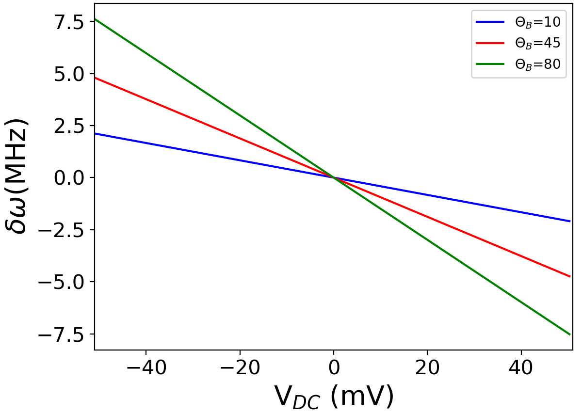
Figure 7: . Shift of the resonance frequency for $B=1$ T, $\lambda=10$ meV, $D=-255$ meV, $F=1.4\lambda$ meV, $k=290eV/{\rm nm}^{2}$ and $d=5\AA$ for three different magnetic field angles.

In Fig. 7 we plot the shift of the resonance frequency as a function of $V_{DC}$ for a Ti-H adatom on MgO. The calculation is carried out with the Hamiltonian Eq. (7). We take $D=-255$ meV, $F=1.4\lambda=14.0$ meV, and $B=1$ T. In order to compute $\delta z$ we take $k=290eV/{\rm nm}^{2}$ and a tip-MgO distance of $d=5\AA$. Yang et al. (2019) The shift scales inversely with $d$. We consider three orientations for $\vec{B}$, forming angles $\theta_{B}=10^{\circ},45^{\circ},80^{\circ}$. Expectedly, the resulting modulation is linear in $V_{DC}$ and the effect is larger for fields off-plane, on account of the fact that $\Delta g_{z}>\Delta g_{x}$. With state of the art STM-ESR, the spectral resolution is around 3MHz. Therefore, the shift might be observed for large values of $V_{DC}$.

The exchange with the tip also contributes to the shift in the ESR frequency Lado et al. (2017); Yang et al. (2017, 2019). Unlike the g factor modulation mechanism, the exchange contribution is tip dependent and decays exponentially with $d$. Therefore, for larger tip-surface distance $d$, the $g$ factor modulation should dominate. Electric shift of the spin resonance was observed experimentally in bulk MgO doped with Cr Royce and Bloembergen (1963), by means of conventional EPR.

XI Discussion and conclusions

The main idea of this paper is that electric fields can modulate the $g$ tensor anisotropy of magnetic adatoms, and that could be used to drive spin transitions. Our work comes motivated by recent ESR-STM experiments Baumann et al. (2015a); Natterer et al. (2017); Choi et al. (2017); Yang et al. (2017); Willke et al. (2018a, b); Bae et al. (2018); Yang et al. (2018, 2019); Willke et al. (2019a). The electric modulation mechanism discussed here is an atomic scale version of the modulation of the $g$ factor of electronsKato et al. (2003); Malissa et al. (2004) and holesPrechtel et al. (2015) in semiconductor nanostructures, that lies at the heart of some well known spintronics Datta and Das (1990) and is becoming a resource in the manipulation of spin qubitsKawakami et al. (2014); Laucht et al. (2015) . At the atomic scale, the modulation proposed here occurs by controlling the weight of two orbital states with $\ell_{z}=\pm 2$, that have a different orbital coupling.

We now briefly discuss some points of our work that could be improved. The derivation of the crystal field parameters for Ti-H/MgO could be improved using a Wannierization Ferrón et al. (2015); Lado et al. (2017). In addition, we could also improve the model Eq. (7) by including the effects of hybridization between the $d$ orbitals of Ti and the $p$ and $s$ orbitals of oxygen and $s$ orbitals of Titanium and Hydrogen, as well as the effect of charge fluctuationsFerrón et al. (2015).

Our estimation of the piezoelectric stretching could be improved in several ways. First, we are treating the silver substrate and most of the MgO as completely rigid. We have verified that keeping the MgO layer completely rigid, or letting a few atoms of the MgO layer close to the Ti adatom relax, has a minor impact on our estimate of $k$. We have also treated the potential as quasi-static. Whereas this is probably a good approximation, it the Gigahertz frequency might resonate with long wavelengths off-plane MgO phonons that would definitely change the Ti-tip distance, very important for the exchange modulation mechanismLado et al. (2017); Yang et al. (2019), and perhaps the Ti-O distance as well.

The $g$ factor observed experimentally for Ti-H/MgO is $g\simeq 1.8$ for magnetic fields pointing almost in plane. From our theory we expect a larger value, closer to $g_{x}=1.97$. There are two possible reasons for this discrepancy. First, the coupling to silver, ignored both in our DFT calculation and in the model, could distort slightly the electronic cloud of Ti-H, which would in turn change $D$ and $F$, and thereby $g_{x}$ and $g_{z}$. Second, and also related to silver, the Kondo coupling to the substrate electrons is expected to renormalize $g$, in analogy to the Knight shiftLangreth and Wilkins (1972); Delgado et al. (2014). In the case of an isotropic interaction, the renormalization of the $g$ factor reads, up to first order in the Kondo exchange between the adatom and the substrate electrons, $J_{s}$:

$$\delta\Delta_{z}=-\frac{\Delta_{z}}{2}g_{s}\rho J_{s}$$ (53)

where $\rho_{s}$ is the density of states of substrate at the Fermi energy and $g_{s}$ is the $g$ factor of the substrate electrons. The sign of $J_{s}$ is positive for antiferromagnetic exchange, which is expected in this system, since Kondo effect was observed for Cu/MgO Yang et al. (2018). Therefore, the Kondo interaction could reduce the $g$ factor of Ti-H.

We now summarize the main results of this work:

1. We have shown that an anisotropic time-dependent modulation of the $g$ tensor induces electronic spin transitions, described by Hamiltonian Eq. (5) and characterized by a Rabi coupling given in Eq. (6).

2. We have worked out an analytical theory for the anisotropic $g$ factor of the Ti-H $S=1/2$ adatom on MgO and we have benchmarked it against DFT calculations. Our theory relates $g$ with crystal field parameters $D$ and $F$, as well as Ti spin orbit coupling $\lambda$ (Eq. (17), Eq. (24) and Fig. 4).

3. We have computed the modulation of the $g$ tensor anisotropy due to the piezoelectric strain of the Ti-H chemisorbed on an oxygen atom on MgO and we have estimated the resulting Rabi coupling (see Fig. 5). We have found that is much smaller than the one observed experimentally, confirming the dominance of the exchange modulation mechanismLado et al. (2017); Yang et al. (2019). However, we have shown that for heavier adatoms with much larger spin orbit coupling $\lambda$, this mechanism could be efficient.

4. We have studied to what extent the crystal field mechanism for ESR-STM, proposed by Baumann et al. to understand the experiments for Fe on MgOBaumann et al. (2015a), could be ascribed to the modulation of the $g$ factor. We find that the dominant contributions to the crystal field mechanism come from the modulation of the zero field splitting parameters.

5. We have also proposed that a DC voltage can shift the $g$ factor, and thereby the Zeeman splitting and we have computed the effect for the case of Ti-H (see Eq. (52) and Fig. 7). This shift provides an additional knob to fine tune the resonance frequency.

6. We have discussed the impact on the hyperfine coupling of the $g$ factor anisotropy and its electric modulation (see Eq. (36)).

7. We have discussed the role of the $g$ factor anisotropy of Ti-H/MgO to enable the exchange-modulation mechanism for ESR-STM (Eq. (50)). In the absence of adatom $g$ factor anisotropy, the exchange-modulation ESR-STM mechanism can only work if the tip moment is not aligned with the applied field (see Eq. (51) ).

In this work we have focused mostly on Ti-H/MgO and Fe/MgO, although most of the ideas can be applied, or extended to the case of other atoms. Most notably, the case of Cu/MgO will be the subject of a future publication.

Acknowledgments We acknowledge Kai Yang, for fruitful discussions. J. F.-R. acknowledges financial support from FCT Grants No. P2020-PTDC/FIS-NAN/4662/2014, UTAP-EXPL/NTec/0046/2017, as well as Generalitat Valenciana funding Prometeo2017/139 and MINECO-Spain (Grant No. MAT2016-78625-C2). A. F. acknowledges hospitality from the Department of Physics of Univeridad de Alicante. A. F., S. A. R. and S. S. G. acknowledge financial support from CONICET (PIP11220150100327, PUE22920170100089CO).

Appendix A Calculation of Rabi constant for spin model

In this appendix we compute the Rabi coupling defined in eq. (5). We consider the general situation for a $S=1/2$:

$${\cal H}=\vec{b}_{0}\cdot\vec{S}_{1}+\vec{b}_{1}(t)\cdot\vec{S}$$ (54)

where

$$\vec{b}_{0}=|\vec{b}_{0}|(\sin\theta_{0},0,\cos\theta_{0})$$ (55)

and

$$\vec{b}_{1}(t)=|\vec{b}_{1}|\cos(2\pi ft)(\sin\theta_{1},0,\cos\theta_{1})$$ (56)

We shall give explicit expressions for $\vec{b}_{0}$ and $\vec{b}_{1}$ below, where we consider independently the exchange modulation and the $g$-factor modulation mechanism.

The eigenstates of $H_{=}\mu_{B}\vec{b}_{0}\cdot\vec{S}$ are, satisfy $H_{0}|\pm\rangle=\pm\mu_{B}|\vec{b}_{0}||\pm\rangle$ and are given by:

$$|+\rangle=\cos\frac{\theta_{0}}{2}|\uparrow\rangle+\sin\frac{\theta_{0}}{2}|\downarrow\rangle$$ (57)

$$|-\rangle=\sin\frac{\theta_{0}}{2}|\uparrow\rangle-\cos\frac{\theta_{0}}{2}|\downarrow\rangle$$ (58)

We obtain the matrix element of the spin operators in the basis of eigenstates:

$$\langle+|S_{x}|-\rangle=\frac{1}{2}\left(\sin^{2}\frac{\theta_{0}}{2}-\cos^{2}\frac{\theta_{0}}{2}\right)=-\frac{1}{2}\cos\theta_{0}$$ (59)

$$\langle+|S_{z}|-\rangle=\sin\frac{\theta_{0}}{2}\cos\frac{\theta_{0}}{2}=\frac{1}{2}\sin\theta_{0}$$ (60)

We can now write the general expression:

$$\Omega=\frac{|\vec{b}_{1}|}{2}\cos(2\pi ft)\left(-\sin\theta_{1}\cos\theta_{0}+\cos\theta_{1}\sin\theta_{0}\right)$$ (61)

This can be further simplified to:

$$\Omega=\frac{|\vec{b}_{1}|}{2}\sin(\theta_{1}-\theta_{0})=\frac{1}{2}\frac{\vec{b}_{0}\times\vec{b}_{1}}{|\vec{b}_{0}|}$$ (62)

A.1 Expression for $\Omega$ for the $g$ factor modulation

We now apply eq. (62) for the case of the $g$ factor modulation. We now write up

$$\vec{b}_{0}=\mu_{B}\left(g_{x}B_{x},0,g_{z}B_{z}\right)$$ (63)

and

$$\vec{b}_{1}=\mu_{B}\left(\delta g_{x}B_{x},0,\delta g_{z}B_{z}\right)$$ (64)

Explicitly, we write:

$$\sin\theta_{0}=\frac{g_{x}B_{x}}{\sqrt{(g_{x}B_{x})^{2}+(g_{z}B_{z})^{2}}}$$ (65)

and

$$\cos\theta_{0}=\frac{g_{z}B_{z}}{\sqrt{(g_{x}B_{x})^{2}+(g_{z}B_{z})^{2}}}$$ (66)

We thus write:

$$\Omega=\frac{\mu_{B}}{2}\left(-\delta g_{x}B_{x}\cos\theta+\delta g_{z}B_{z}\sin\theta\right)$$ (67)

We now use eq. (65) and (66) to express $B_{x}$ and $B_{y}$ in terms of $\theta,g_{x},g_{z},B_{x},B_{z}$ and we obtain:

$$\Omega=\frac{\mu_{B}}{2}|\vec{b}_{0}|\cos\theta_{0}\sin\theta_{0}\left(-\frac{\delta g_{x}}{g_{x}}+\frac{\delta g_{z}}{g_{z}}\right)$$ (68)

Now we use $\cos\theta_{0}\sin\theta_{0}=\frac{1}{2}\sin 2\theta_{0}$ to obtain:

$$\Omega=\frac{\mu_{B}}{4}|\vec{b}_{0}|\sin 2\theta_{0}\left(\frac{\delta g_{z}}{g_{z}}-\frac{\delta g_{x}}{g_{x}}\right)$$ (69)

We now write the Zeeman splitting

$$\Delta_{Z}=\mu_{B}|\vec{b}_{0}|$$ (70)

so that we obtain the expression:

$$\Omega=\frac{\Delta_{Z}}{4}\sin 2\theta\left(\frac{\delta g_{z}}{g_{z}}-\frac{\delta g_{x}}{g_{x}}\right)$$ (71)

A.2 Expression for $\Omega$ for the exchange modulation

We now consider a Hamiltonian for a $S=1/2$ surface spin where, in addition to the Zeeman interaction, there is a exchange coupling to the magnetic moment of the tip:

$${\cal V}_{\rm exch}=J(z)\vec{n}_{T}\cdot\vec{S}$$ (72)

where

$$\vec{n}_{T}=\left(\cos(\theta_{B}+\delta),0,\sin(\theta_{B}+\delta)\right)$$ (73)

and $\vec{B}=B_{0}\left(\cos(\theta_{B}),0,\sin(\theta_{B})\right)$

We define the spin splitting

$$\Delta_{Z}^{*}\equiv\sqrt{(g_{x}\mu_{B}B_{x}+Jn_{x})^{2}+(g_{z}\mu_{B}B_{z}+Jn_{z})^{2}}$$ (74)

and we express the angles as

$$\sin\theta_{0}=\frac{g_{x}B_{x}+Jn_{x}}{\Delta_{Z}^{*}}$$ (75)

and

$$\cos\theta_{0}=\frac{g_{z}B_{z}+Jn_{z}}{\Delta_{Z}^{*}}$$ (76)

For the time dependent component, we now ignore the modulation of the $g$ factors and we only consider the modulation of the exchange, that we write up as $\delta J\cos 2\pi ft$. We thus can write

$$\vec{b}_{1}(t)=\delta J\left(n_{x},0,n_{z}\right)$$ (77)

After some algebra we obtain:

$$\Omega_{J}=\frac{\delta J}{2\Delta_{z}^{*}}\left(g_{x}\mu_{B}.B_{x}n_{z}-g_{z}\mu_{B}B_{z}n_{x}\right)$$ (78)

Since we are interested in the role of the $g$ factor anisotropy, we make it explicit and we write:

$$g_{x}=g+\Delta g_{x}$$

$$g_{z}=g+\Delta g_{z}$$ (79)

where $\Delta g_{x}$ and $\Delta g_{z}$ are the static contributions to the $g$ factor anisotropy. We now define

$${\cal E}_{J}\equiv\frac{\delta J}{2\Delta_{z}^{*}}g\mu_{B}B$$ (80)

so that the expression for the Rabi reads:

$$\Omega_{J}={\cal E}_{J}\left(\cos\theta_{B}\sin(\theta_{B}+\delta)-\sin\theta_{B}\cos(\theta_{B}+\delta)\right)+$$

$${\cal E}_{J}\left(\frac{\Delta g_{x}}{g}\cos\theta_{B}\sin(\theta_{B}+\delta)-\frac{\Delta g_{z}}{g}\sin\theta_{B}\cos(\theta_{B}+\delta)\right)$$

We can now write this up as:

$$\Omega_{J}={\cal E}_{J}\sin\delta+$$

$${\cal E}_{J}\left(\frac{\Delta g_{x}}{g}\cos\theta_{B}\sin(\theta_{B}+\delta)-\frac{\Delta g_{z}}{g}\sin\theta_{B}\cos(\theta_{B}+\delta)\right)$$

After some algebra we obtain:

$$\Omega_{J}={\cal E}_{J}\sin\delta+$$

$${\cal E}_{J}\left(\frac{\Delta g_{x}}{g}-\frac{\Delta g_{z}}{g}\right)\cos\theta_{B}\sin\theta_{B}\cos\delta+$$

$$+{\cal E}_{J}\left(\frac{\Delta g_{x}}{g}\cos^{2}\theta_{B}+\frac{\Delta g_{z}}{g}\sin^{2}\theta_{B}\right)\sin\delta$$ (81)

Appendix B Estimation of SOC from NIST Database

From the NIST databaseKelleher et al. (1999), we obtain the experimental values for Ti(IV) with an outermost electronic configuradion $d^{1}$. The lowest energy levels have $L=2$ and $S=1/2$, with $J=3/2$ and $J=5/2$. Their energy splitting is $\Delta E=47.3$ meV. We can relate this to the spin orbit coupling using $J=L+S$ and:

$$\lambda\vec{L}\cdot\vec{S}=\frac{\lambda}{2}\left(J(J+1)-L(L+1)-S(S+1)\right)$$ (82)

From here we obtain:

$$E(J)=\frac{\lambda}{2}\left(J(J+1)-L(L+1)-S(S+1)\right)$$ (83)

and

$$E(J+1)-E(J)=\frac{\lambda}{2}\left(J+1(J+2-J)\right)=(J+1)\lambda$$ (84)

Since $J+1=\frac{5}{2}$ we obtain $\lambda_{IV}=\frac{2}{5}\Delta E_{IV}=18.9$ meV. If we consider Ti(III), we have $J+1=3$ and $\Delta E_{III}=22.9$meV. This yields $\lambda_{IV}=\frac{1}{3}\Delta E_{III}=7.63$

It is apparent that the strength of the atomic spin orbit coupling depends on the charge imbalance in the Ti. One can expect that value of $\lambda$ for Ti-H on MgO must be in between these two values.

Appendix C Relation between the $(\ell^{+})^{4}+(\ell^{-})^{4}$ and the $\ell_{x}^{4}+\ell_{y}^{4}$ terms

In this appendix we discuss the connection between these two crystal field operators, that we have used for Ti and Fe. The choice is a matter of convenience. After some algebra, the relation between these two operators is

$$\ell_{x}^{4}+\ell_{y}^{4}=\frac{(\ell^{+})^{4}+(\ell^{-})^{4}}{8}+24I-\frac{91}{12}\ell_{z}^{2}+\frac{7}{12}\ell_{z}^{4}$$ (85)

Thus, it is apparent that the last two terms can can be reabsorbed as a renormalization of the $D\ell_{z}^{2}$ term, plus a shift of the $\ell_{z}=0$ level, that plays a very minor role in the discussion for Ti-H/MgO.

References

- Manassen et al. (1989) Y. Manassen, R. J. Hamers, J. E. Demuth, and A. J. Castellano Jr., Phys. Rev. Lett. 62, 2531 (1989), URL http://link.aps.org/doi/10.1103/PhysRevLett.62.2531.
- Balatsky et al. (2012) A. V. Balatsky, M. Nishijima, and Y. Manassen, Advances in Physics 61, 117 (2012).
- Baumann et al. (2015a) S. Baumann, W. Paul, T. Choi, C. P. Lutz, A. Ardavan, and A. J. Heinrich, Science 350, 417 (2015a).
- Natterer et al. (2017) F. D. Natterer, K. Yang, W. Paul, P. Willke, T. Choi, T. Greber, A. J. Heinrich, and C. P. Lutz, Nature 543, 226 (2017).
- Choi et al. (2017) T. Choi, W. Paul, S. Rolf-Pissarczyk, A. J. Macdonald, F. D. Natterer, K. Yang, P. Willke, C. P. Lutz, and A. J. Heinrich, Nature nanotechnology 12, 420 (2017).
- Yang et al. (2017) K. Yang, Y. Bae, W. Paul, F. D. Natterer, P. Willke, J. L. Lado, A. Ferrón, T. Choi, J. Fernández-Rossier, A. J. Heinrich, et al., Physical review letters 119, 227206 (2017).
- Willke et al. (2018a) P. Willke, W. Paul, F. D. Natterer, K. Yang, Y. Bae, T. Choi, J. Fernández-Rossier, A. J. Heinrich, and C. P. Lutz, Science advances 4, eaaq1543 (2018a).
- Willke et al. (2018b) P. Willke, Y. Bae, K. Yang, J. L. Lado, A. Ferrón, T. Choi, A. Ardavan, J. Fernández-Rossier, A. J. Heinrich, and C. P. Lutz, Science 362, 336 (2018b).
- Bae et al. (2018) Y. Bae, K. Yang, P. Willke, T. Choi, A. J. Heinrich, and C. P. Lutz, Science advances 4, eaau4159 (2018).
- Yang et al. (2018) K. Yang, P. Willke, Y. Bae, A. Ferrón, J. L. Lado, A. Ardavan, J. Fernández-Rossier, A. J. Heinrich, and C. P. Lutz, Nature nanotechnology 13, 1120 (2018).
- Yang et al. (2019) K. Yang, W. Paul, F. D. Natterer, J. L. Lado, Y. Bae, P. Willke, T. Choi, A. Ferrón, J. Fernández-Rossier, A. J. Heinrich, et al., Physical Review Letters 122, 227203 (2019).
- Willke et al. (2019a) P. Willke, K. Yang, Y. Bae, A. J. Heinrich, and C. P. Lutz, Nature Physics p. 1 (2019a).
- Willke et al. (2019b) P. Willke, A. Singha, X. Zhang, T. Esat, C. P. Lutz, A. J. Heinrich, and T. Choi, arXiv preprint arXiv:1908.11061 (2019b).
- Natterer et al. (2019) F. D. Natterer, F. Patthey, T. Bilgeri, P. R. Forrester, N. Weiss, and H. Brune, Review of Scientific Instruments 90, 013706 (2019).
- Seifert et al. (2019) T. Seifert, S. Kovarik, C. Nistor, L. Persichetti, S. Stepanow, and P. Gambardella, arXiv preprint arXiv:1908.03379 (2019).
- Thiele et al. (2014) S. Thiele, F. Balestro, R. Ballou, S. Klyatskaya, M. Ruben, and W. Wernsdorfer, Science 344, 1135 (2014).
- Godfrin et al. (2017) C. Godfrin, A. Ferhat, R. Ballou, S. Klyatskaya, M. Ruben, W. Wernsdorfer, and F. Balestro, Physical review letters 119, 187702 (2017).
- Rashba (1960) E. I. Rashba, Soviet Physics, Solid State 2, 1109 (1960).
- Kato et al. (2003) Y. Kato, R. Myers, D. Driscoll, A. Gossard, J. Levy, and D. Awschalom, Science 299, 1201 (2003).
- Tokura et al. (2006) Y. Tokura, W. G. van der Wiel, T. Obata, and S. Tarucha, Phys. Rev. Lett. 96, 047202 (2006), URL http://link.aps.org/doi/10.1103/PhysRevLett.96.047202.
- Pioro-Ladriere et al. (2008) M. Pioro-Ladriere, T. Obata, Y. Tokura, Y.-S. Shin, T. Kubo, K. Yoshida, T. Taniyama, and S. Tarucha, Nature Physics 4, 776 (2008).
- Bell (1962) R. L. Bell, Phys. Rev. Lett. 9, 52 (1962), URL https://link.aps.org/doi/10.1103/PhysRevLett.9.52.
- George et al. (2013) R. E. George, J. P. Edwards, and A. Ardavan, Phys. Rev. Lett. 110, 027601 (2013), URL https://link.aps.org/doi/10.1103/PhysRevLett.110.027601.
- Hoffman (1994) B. M. Hoffman, The Journal of Physical Chemistry 98, 11657 (1994).
- Berggren and Fransson (2016) P. Berggren and J. Fransson, Scientific reports 6, 25584 (2016).
- Lado et al. (2017) J. L. Lado, A. Ferrón, and J. Fernández-Rossier, Physical Review B 96, 205420 (2017).
- Shakirov et al. (2019) A. M. Shakirov, A. N. Rubtsov, and P. Ribeiro, Physical Review B 99, 054434 (2019).
- Gálvez et al. (2019) J. R. Gálvez, C. Wolf, F. Delgado, and N. Lorente, Physical Review B 100, 035411 (2019).
- Giannozzi et al. (2009) P. Giannozzi, S. Baroni, N. Bonini, M. Calandra, R. Car, C. Cavazzoni, D. Ceresoli, G. L. Chiarotti, M. Cococcioni, I. Dabo, et al., Journal of physics: Condensed matter 21, 395502 (2009).
- Perdew et al. (1998) J. Perdew, K. Burke, and M. Ernzerhof, Physical Review Letters 80, 891 (1998).
- Blöchl (1994) P. E. Blöchl, Physical review B 50, 17953 (1994).
- Pickard and Mauri (2002) C. J. Pickard and F. Mauri, Physical review letters 88, 086403 (2002).
- Baumann et al. (2015b) S. Baumann, W. Paul, T. Choi, C. P. Lutz, A. Ardavan, and A. J. Heinrich, Science 350, 417 (2015b).
- Baumann et al. (2015c) S. Baumann, F. Donati, S. Stepanow, S. Rusponi, W. Paul, S. Gangopadhyay, I. G. Rau, G. E. Pacchioni, L. Gragnaniello, M. Pivetta, et al., Phys. Rev. Lett. 115, 237202 (2015c).
- Klein (1952) M. J. Klein, Am. J. Phys. 20, 65 (1952).
- Garg (1993) A. Garg, EPL (Europhysics Letters) 22, 205 (1993).
- Wernsdorfer and Sessoli (1999) W. Wernsdorfer and R. Sessoli, Science 284, 133 (1999).
- Delgado et al. (2015) F. Delgado, S. Loth, M. Zielinski, and J. Fernández-Rossier, EPL (Europhysics Letters) 109, 57001 (2015).
- George et al. (2010) R. E. George, W. Witzel, H. Riemann, N. V. Abrosimov, N. Nötzel, M. L. W. Thewalt, and J. J. L. Morton, Phys. Rev. Lett. 105, 067601 (2010).
- Shafiei et al. (2013) M. Shafiei, K. C. Nowack, C. Reichl, W. Wegscheider, and L. M. K. Vandersypen, Phys. Rev. Lett. 110, 107601 (2013), URL https://link.aps.org/doi/10.1103/PhysRevLett.110.107601.
- Royce and Bloembergen (1963) E. B. Royce and N. Bloembergen, Phys. Rev. 131, 1912 (1963), URL https://link.aps.org/doi/10.1103/PhysRev.131.1912.
- Malissa et al. (2004) H. Malissa, W. Jantsch, M. Mühlberger, F. Schäffler, Z. Wilamowski, M. Draxler, and P. Bauer, Applied physics letters 85, 1739 (2004).
- Prechtel et al. (2015) J. H. Prechtel, F. Maier, J. Houel, A. V. Kuhlmann, A. Ludwig, A. D. Wieck, D. Loss, and R. J. Warburton, Physical Review B 91, 165304 (2015).
- Datta and Das (1990) S. Datta and B. Das, Applied Physics Letters 56, 665 (1990).
- Kawakami et al. (2014) E. Kawakami, P. Scarlino, D. R. Ward, F. Braakman, D. Savage, M. Lagally, M. Friesen, S. N. Coppersmith, M. A. Eriksson, and L. Vandersypen, Nature nanotechnology 9, 666 (2014).
- Laucht et al. (2015) A. Laucht, J. T. Muhonen, F. A. Mohiyaddin, R. Kalra, J. P. Dehollain, S. Freer, F. E. Hudson, M. Veldhorst, R. Rahman, G. Klimeck, et al., Science advances 1, e1500022 (2015).
- Ferrón et al. (2015) A. Ferrón, F. Delgado, and J. Fernández-Rossier, New Journal of Physics 17, 033020 (2015).
- Ferrón et al. (2015) A. Ferrón, J. L. Lado, and J. Fernández-Rossier, Phys. Rev. B 92, 174407 (2015).
- Langreth and Wilkins (1972) D. C. Langreth and J. W. Wilkins, Physical Review B 6, 3189 (1972).
- Delgado et al. (2014) F. Delgado, C. Hirjibehedin, and J. Fernández-Rossier, Surface Science 630, 337 (2014).
- Kelleher et al. (1999) D. E. Kelleher, W. C. Martin, W. L. Wiese, J. Sugar, J. R. Fuhr, K. Olsen, A. Musgrove, P. J. Mohr, J. Reader, and G. Dalton, Physica Scripta 1999, 158 (1999).