Hartle-Hawking boundary conditions as Nucleation by de Sitter Vacuum

Abstract

It is shown that, for a de Sitter Universe, the Hartle-Hawking (HH) wave function can be obtained in a simple way starting from the Friedmann-Lemaitre-Robertson-Walker (FLRW) line element of cosmological equations. An oscillator having imaginary time is indeed derived starting from the Hamiltonian obtaining the HH condition. This proposes again some crucial matter on the meaning of complex time in cosmology. In order to overcome such difficulties, we propose an interpretation of the HH framework based on de Sitter Projective Holography.

¹Department of Physics, University of Trieste, via Valerio 2, 34127 Trieste, Italy

²Research Institute for Astronomy and Astrophysics of Maragha (RIAAM), P.O. Box 55134-441, Maragha, Iran and International Institute for Applicable Mathematics and Information Sciences, B. M. Birla Science Centre, Adarshnagar, Hyderabad 500063, India

PhySH:

Gravitation, Cosmology & Astrophysics/Cosmology/Quantum Cosmology.

Keywords:

Hartle-Hawking wave function; de Sitter Projective Holography; complex time; quantum oscillator.

1 Introduction

The Hartle-Hawking (HH) proposal of “no boundary conditions” [1] is, till now, the most powerful and fruitful theory on the original quantum state of the Universe. Its original motivation was to avoid the initial singularity of the Universe due to the cosmological application of the general theory of relativity (GTR) [10]. The HH proposal concerns the state of the Universe before the Planck time, that is, before the emerging of the classical space-time by an overlapping of quantum patterns [1]. Such an emerging is realized through a functional on the geometries of compact three-manifolds and on the values of the matter-fields on such manifolds [1]. In that way, the wave function of the Universe’s ground state is obtained by a path integral over all compact positive-definite four-geometries having the three-geometry as a boundary [1]. It implies a constraint on the Hermitian behavior of the Hamiltonian which satisfies the famous Wheeler-DeWitt wave equation for the Universe and enables its computability [11]. After the initial HH proposal, the no boundary conditions have been discussed in other, different scenarios like multiverse, brane world, inflation, quantum potential [12-15]. In such works, it is assumed that the “vacuum” before the Big-Bang represents the absence of a classical space-time. An interesting question concerns if such an assumption of absence of a classical space-time works beyond cosmology, maybe including the whole realm of quantum theory [16]. Some recent foundational scenarios go in the same direction [17, 18]. In this work, the HH proposal is reanalysed starting from its recent generalization in [19]. In Section 2, a way to construct the Lagrangian starting from the Friedmann-Lemaitre-Robertson-Walker (FLRW) line element is considered and an oscillator having imaginary time is derived starting from the Hamiltonian obtaining the HH condition. In Section 3 we discuss some problem of de Sitter geometry. In Section 4 we focus on the meaning of the derived oscillator within a de Sitter framework with a bird view vision on de Sitter Projective Cosmology. Finally, we will conclude with a discussion concerning time and wave function in cosmology.

2 A Cosmological Lagrangian for the Hartle-Hawking conditions

In the recent work [19], Hartle and collaborators reconsidered the nature of the no-boundary conditions. In that way, they proposed a generalization which should facilitate the understanding of the HH proposal and its application to observational studies of the Universe. The basic idea in [19] is that the HH proposal arises from a semi-classical constraint which results completely independent by specific assumptions on the real nature of the quantum theory of gravity. This is different with respect to the pioneering papers by Hawking and collaborators where the path integrals approach has been applied to quantum fluctuations, see for example [20, 21]. In fact, in such works the connection between path integrals and euclidean geometry was not only considered in terms of a constructive approach, but also as a possible connection with quantum gravity based on its specific application to black hole radiance. This generated various problems also in the semi-classical approach to the no-boundary wave function (NBWF) through tunnelling effect, which was been introduced by Vilenkin [22, 23]. In a remarkable paper [24], Lehners and Turok has shown that, for a large class of theories, a semi-classical approach to the NBWF through path integrals is incompatible with the Euclidean approach. The Euclidean issue, which will be partially discussed also in the present paper, is very controversial, see for example [25].

In [19], the NBWF has been assumed to be the Universe’s ground state and the authors have shown that path integrals are not needed if one uses general assumptions. The most important among such assumptions are the compatibility between the GTR and quantum mechanics (QM) and the definition of the wave function by a collections of saddle points which guarantee the opportune smoothness between the quantum ground state and the subsequent evolution of the space-time.

In the present work, it is chosen to construct the wave function starting from the Universe’s scale factor through a quantum-like approach. After that, it will be shown that such a wave function satisfies the HH no-boundary condition.

The starting point is to construct a Lagrangian from the scale factor of the Universe, which gives the FLWR equations [3]. Let us consider the following Lagrangian for a homogeneous and isotropic Universe:

$$L(R,\dot{R})=\dot{R}^{2}+\frac{8\pi G\rho}{3}R^{2}+\frac{\Lambda c^{2}}{3}R^{2},$$ (1)

where $R=R(t)$, $\rho=\rho(R)$ is the energy density of matter in the Universe, and $\Lambda$ is the cosmological constant introduced by Einstein in 1917 [4]. Starting from Eq. (1), one derives the first FLRW equation. One considers the scale factor $R$ as being a generalized coordinate. Then, the energy of the Universe is:

$$E(R,\dot{R})=\left(\frac{\partial L}{\partial\dot{R}}\right)\dot{R}-L=\dot{R}^{2}-\frac{8\pi G\rho}{3}R^{2}-\frac{\Lambda c^{2}}{3}R^{2}.$$ (2)

This energy is constant because the Lagrangian does not depend explicitly on time [5]. Denoting the constant $E$ by $-kc^{2}$, one obtains

$$\left(\frac{\dot{R}}{R}\right)^{2}+\frac{kc^{2}}{R^{2}}=\frac{8\pi G\rho}{3}+\frac{\Lambda c^{2}}{3}.$$ (3)

This equation is the first equation for the standard Lambda-CDM model [6], which can be closed ($k=1$), flat ($k=0$), or open ($k=-1$) [3]. In order to get a unit of energy, one multiplies the Lagrangian (1) by a constant mass:

$$L(R,\dot{R})=m\left(\dot{R}^{2}+\frac{8\pi G\rho}{3}R^{2}+\frac{\Lambda c^{2}}{3}R^{2}\right).$$ (4)

From the above relations the Hamiltonian can be written down as

$$H(R,\dot{R})=\frac{1}{2}m\dot{R}^{2}-\frac{4\pi mG\rho}{3}R^{2}-\frac{\Lambda mc^{2}}{6}R^{2}.$$ (5)

We consider a pure de Sitter Universe, which simplifies the Lambda-CDM Cosmology by modelling the Universe as spatially flat and neglects ordinary matter [7]. Thus, the dynamics of the Universe are dominated by the cosmological constant, which should correspond to Dark Energy in the present Universe or to the inflaton field in the early Universe. In this case, the first Friedmann equation becomes:

$$\left(\frac{\dot{R}}{R}\right)^{2}=\frac{\Lambda c^{2}}{3},$$ (6)

and the Hamiltonian

$$H(R,\dot{R})=\frac{1}{2}m\dot{R}^{2}-\frac{\Lambda mc^{2}}{6}R^{2}.$$ (7)

Following [56], one constructs a phase space $(R,P_{R})$, where $R$ is the comoving coordinate with

$$P_{R}=m\dot{R}$$ (8)

being the linear momentum. Thus, inserting Eq. (8) into Eq. (7), one obtains

$$H(R,\dot{R})=\frac{P_{R}^{2}}{2m}-\frac{\Lambda mc^{2}}{6}R^{2}.$$ (9)

Therefore, one goes ahead with the canonical quantization [8]

$$P_{R}\rightarrow\mathcal{P_{R}}=-i\hbar\frac{\partial}{\partial R},$$ (10)

obtaining the Hamiltonian operator

$$\mathcal{H}=-\frac{\hbar^{2}}{2m}\frac{\partial^{2}}{\partial R^{2}}-\frac{\Lambda mc^{2}}{6}R^{2}.$$ (11)

Rescaling $\Lambda$ and setting $\hbar=c=m=1,$ one gets

$$\mathcal{H}=\frac{1}{2}(\mathcal{P_{R}}^{2}-\Lambda R^{2}).$$ (12)

which is exactly the Hamiltonian of a simple harmonic oscillator. The frequency is determined by $\sqrt{\Lambda}$. At this point, one considers three cases of interest: $\Lambda=0$ (free particle), $\Lambda<0$ (oscillator) and $\Lambda>0$ (inverted oscillator). Firstly, let us consider the case $R\in(0,\infty)$. The obvious choice for the Hilbert space is $L^{2}(\mathbb{R^{+}},dR)$. In this space the Hamiltonians of the form $\mathcal{P_{R}}^{2}+V(R)$ have self-adjoint extensions [8]. Specifically, it is readily checked that the physical Hamiltonian (12) is symmetric in the usual representation $\mathcal{P_{R}}^{2}\rightarrow-i\frac{\partial}{\partial R}$, provided $\lim_{x\rightarrow\infty}\phi=0$ and $\lim_{x\rightarrow 0}[\psi^{*}\phi-\phi\psi^{*}]=0$. This gives the boundary condition $\phi^{\prime}(0)=\alpha\phi(0),\alpha\in\mathbb{R}$. The Hilbert space is the subspace specified by

$$\mathbb{H_{\alpha}}=\left\{\phi\in L^{2}(\mathbb{R^{+}},dR)\right\}.$$ (13)

Following [9], one solves the time-dependent Schrödinger equation

$$i\frac{\partial}{\partial t}\phi(R,t)=-\frac{1}{2}\frac{\partial^{2}}{\partial R^{2}}\phi(R,t)-\frac{1}{2}\Lambda R^{2}\phi(R,t),$$ (14)

with the above mentioned boundary condition.

If $\Lambda=0$, there are two types of elementary solutions: ingoing and outgoing waves of fixed energy and a bound state. The first one, satisfying the above boundary condition, has the form

$$\phi_{\alpha k}(R,t)=e^{ik^{2}t/2}\left[e^{ikR}-\left(\frac{\alpha-ik}{\alpha+ik}\right)e^{-ikR}\right].$$ (15)

Concerning the second type of solution, a bound state, one gets

$$\phi(R,t)=e^{i\textmd{k}^{2}t/2}e^{-\textmd{k}R},\hskip 14.22636pt\textmd{k}>0.$$ (16)

In the case of $\Lambda<0$ (AdS Universe), one has the oscillator on the half-line with the usual boundary condition. With $\Lambda=-1/l^{2}$ and $\zeta=t/l$, the propagator on $\mathbb{R}$ is

$$K(R,\zeta,R^{\prime},0)=\sqrt{\frac{1}{2\pi il\sin(\zeta)}}\exp\left\{\frac{i[(R^{2}+R^{\prime 2})\cos(\zeta)-2RR^{\prime}]}{2l\sin(\zeta)}\right\}.$$ (17)

Now, let us consider the region $R<0$. Given $\psi(R,0)=f(R)$ for $x>0$, the initial data $f(R)$ on $\mathbb{R^{+}}$ can be extended to the region $R<0$, such that

$$f^{\prime}(R)-\alpha f(R)=-(f^{\prime}(-R)-\alpha f(-R)),\hskip 14.22636ptR<0,$$ (18)

that is, imposing antisymmetry on the boundary condition function. If one solves this equation, one obtains the required extension

$$f_{L}(R)\equiv e^{\alpha R}\int_{R}^{0}e^{-\alpha u}f^{\prime}(-u)-\alpha f(-u)\,du+e^{\alpha R}f(0),\hskip 14.22636ptR<0,$$ (19)

where the integration constant is chosen such that $f_{L}(0)=f(0)$. Convoluting the data so extended with the full-line propagator (17), one gets the solution

$$\psi(R,\zeta)=\int_{-\infty}^{0}K(R,\zeta,R^{\prime},0)f_{L}(R^{\prime})\,dR^{\prime}+\int_{0}^{\infty}K(R,\zeta,R^{\prime},0)f(R^{\prime})\,dR^{\prime},\hskip 14.22636ptR>0.$$ (20)

If $\Lambda<0$, the Hamiltonian is not bounded below. However the unitary evolution operator is still well defined since the Hamiltonian has self-adjoint extensions. The propagator on $\mathbb{R}$ is obtained by the replacement $l\rightarrow il$ to give

$$\bar{K}(R,\zeta,R^{\prime},0)=\sqrt{\frac{1}{2\pi il\sinh(\zeta)}}\exp\left\{\frac{i[(R^{2}+R^{\prime 2})\cosh(\zeta)-2RR^{\prime}]}{2l\sinh(\zeta)}\right\}.$$ (21)

Starting from this expression, setting $R^{\prime}=0$, one obtains the HH wave function:

$$\Psi_{HH}\equiv\bar{K}(R,\zeta,0,0)=\sqrt{\frac{1}{2\pi il\sinh(\zeta)}}\exp\left\{-\frac{iR^{2}}{2l\tanh(\zeta)}\right\}.$$ (22)

It is a remarkable issue that, starting from a series of simple and quantum-like assumptions, one can get the HH wave function, with the important interpretative contribution of the harmonic oscillator of Eq. (12) (another approach can be found in [9]). Thus, our analysis seems to confirm the well known statement by Sidney Coleman that "The career of a young theoretical physicist consists of treating the harmonic oscillator in ever-increasing levels of abstraction" [26]. The issue that one can obtain HH from Eq. (12) is consistent with the idea of Vilenkin on the presence of a tunnelling effect [22, 23]. In addition, one observes that the frequency of the oscillator depends on the cosmological constant. This can suggest a special role of $\Lambda$, which goes well beyond the large-scale geometrical structure. We will further discuss this special role of $\Lambda$ in the following of the paper.

3 Problems with de Sitter geometry

Now, let us ask if the physical interpretation of the HH function can be considered exhaustive or, alternatively, if we still need some further conceptual tessera. In fact, the interpretation of QM in a cosmological framework needs particular rules. It is sufficient recalling that the whole array of matters connected to the role of the observer (like preparing a quantum state and its measures) does not work in quantum cosmology. This is efficaciously stressed by R. Serber "Observers were not present at the Big-Bang instant" [27]. This generated an interesting, hot debate with various opposing opinions, on one hand, on the cosmological perspectives of different approaches (de Broglie-Bohm theory, Decoherent Histories Approach to Quantum Mechanics, Everettian Many Worlds); on the other hand on the role of some fundamental rule of “quantum data”, like the Born Rule [28, 29]. A very important issue is that, generally speaking, QM, with its various interpretations, refers to a space-time where the wave function evolves. On the contrary, in quantum cosmology the wave function generates the same space-time. In fact, the origin of quantum cosmology basically arises from attempts to remove the classical initial singularity at the quantum level and from a starting point to study the "subtle fabric" of quantum gravity. Thus, researchers have a general agreement only on few issues, but such few issues are sufficient in order to understand that, beyond its formal fineness, quantum cosmology is still at an early stage where one has no definitive interpretations because the old problem of the “Peaceful Coexistence” between the Classical Space-Time and the Quantum Realm is still present and very strong [30].

Concerning our discussion on the HH wave function, a suggestive way to describe the physical situation is telling that one finds a “quantum nebula” which replaces the classical initial singularity. This “quantum nebula” generates an accelerate expansion of the space-time structure. This has not to be considered "a collapse". Instead, it is a kind of natural smooth transition which is completely unprecedented in QM. In addition, one must consider a metric structure as being the description of a physical field on a fixed background (usually, that background has constant curvature) [31]. Hence, the main task of the HH wave function is to produce the collapse of a very high number of freedom degrees of quanta through a kind of “nucleation”. In other words, a space-time which is described by a differentiable manifold is an emergent phenomenon while the metric and the Christoffell connections are collective variables which can work only at lows energies and long wavelengths. This approach concerns some recent theories of superfluid vacuum [32, 33], while, in the recent work [18], a unitary approach to both the particle-like "Little Bangs" and the cosmological "Big-One" where the wave function is always interpreted as an event-based emergent phenomenon has been proposed. The oscillator (12) seems a natural answer to the idea of nucleation and a potential strong connection with the value of the cosmological constant appears to be a logical consequence of the approach of this paper. Thus, problems concerning the physical interpretation of the HH wave function are transferred to the oscillator (12) which works with imaginary time. Actually, this issue revealed itself in the original derivation of the HH wave function [1]. The “quantum nebula” is indeed technically described by Hartle & Hawking in terms of a de Sitter-like Universe having imaginary time. In this framework, space and time are indistinguishable and close to each other. Hawking and collaborators stressed in various works (see for example [34]) that the subsequent parallel sections of that hypersphere should represent a hyperspherical, three-dimensional space which starts from a non-singular “South Pole”. This pole expands as far as a maximum dimension and, after that, it reduces to a “North Pole”, which is still non-singular as the global space has a hyperspherical behavior. This idea came first the cosmological evidence of an accelerating Universe with the triumphant comeback of the cosmological constant, but it represents the essence of the line of reasoning of Hawking and collaborators. The problem is that such a line of reasoning seems erroneous. In fact, if one assumes that imaginary time is portrayed by a maximum circle, the spatial sections, which are perpendicular to the points of the circle, are S3 space having constant section! Then, in the absence of a “collapse” (or some exotic mechanism), one cannot understand in which way a de Sitter Universe having imaginary time becomes a FLRW Universe having real time. On the other hand, it is exactly a de Sitter hyperspherical Universe having imaginary time, with its new, central position in cosmology, which tells one that the HH approach is an intriguing idea which opens to various interesting possibilities. Here, we propose an alternative method in order to analyse de Sitter Universe, which is based on the approach of the so called de Sitter Projective Relativity [35]. We think that in this scenario the HH wave function and the oscillator (12) can find a new, enlightening interpretation.

4 The Physical Meaning of Complex Time in de Sitter Projective Holography

The Theory of de Sitter Projective Holography was born within a program of Quantum Cosmology and has also developed a new approach to Particle Physics [36 - 40]. For our purpose, it suffices here to define Vacuum as a Universal Action Reservoir [41] placed on a 4D surface of an Euclidean five-dimensional (5D) hypersphere. This surface can be converted into a 4D hyperboloid which represents a de Sitter space–time by a Wick rotation. The Beltrami projective representation of this de Sitter space–time on a 4D hyperplane tangent to the hyperboloid in the point-event of observation is known as “Castelnuovo chronotope.” It is important to remark that the group approach [42, 43] makes possible to individuate the de Sitter Universe as a framework of physical processes without referring to any “local” physics. The de Sitter group is in fact the simplest 4D group containing those of Galilei and Lorentz-Poincaré. We note that it is not necessary to imagine the hypersphere as an “enlarged” space-time. The space-time labels of observable events do not belong to the archaic phase, represented on the hypersphere: it is populated with virtual processes only. We called such theory “Archaic” because the role of the hypersphere and that of the observed Universe are not related by a “before” and an “after”. The hypersphere is rather like a highly non-local, a-temporal phase. The space-time positions or “labels” are, instead, related to the descriptions of the classes of observers on the tangent $P^{4}$-plane (Beltrami-Castelnuovo Projective representation, see figure 4.1).

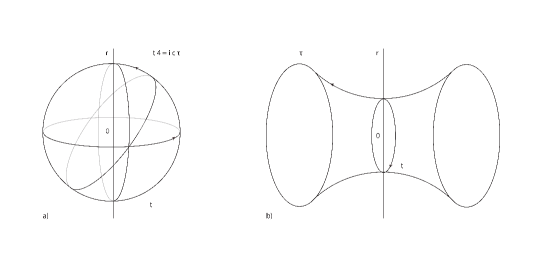
Figure 4.1: Beltrami-Castelnuovo Projective representation: a) imaginary time and b) real time.

The passage from a description to the other one is defined by the Wick rotation [44]: before jumping out from vacuum, particles are in a virtual status described by the imaginary time of pre-space; during the observable existence lag, the real time comes into play. The manifestation of particles from the vacuum and their disappearance into the vacuum are the real microinteractions described in quantum theory through the wave-function “collapse” or reduction (R processes). To all effects, a “localization” at the level of individual event in microphysics, a “nucleation” in the case of the Big Bang. Such strong unity between macro and microphysics justifies the consideration of an archaic holography ruled by a Wick rotation and projectivity. Now, let us take a closer look at the role of imaginary time. We can think of an axis $\underline{x}_{0}$ of the hypersphere representing inverse temperatures, and imagine that below a critical value of this coordinate the physical processes are constrained to remain virtual. This constraint is removed when $\underline{x}_{0}$ exceeds the critical value, thus permitting the emergence of real processes in real time, at a rate completely analogous to the exponential one of the radioactive decay. This axis can be considered as an “archaic precursor” of time. The 5-sphere is:

$$(\underline{x}_{0})^{2}+(\underline{x}_{1})^{2}+(\underline{x}_{2})^{2}+(\underline{x}_{3})^{2}+(\underline{x}_{5})^{2}=r^{2}.$$ (23)

It is reasonable to assume the critical value as corresponding to baryogenesis temperature:

$$T_{C}=\frac{\hbar}{k\theta_{0}},$$ (24)

where $\theta_{0}\sim 10^{-23}$ s plays the role of the fundamental time interval (chronon), so $T_{C}\approx 10^{13}$ K. We will come back later on the chronon and its relations with timescales. One can believe, without too much effort, that even in the archaic phase the state of matter could still be described by means of macroscopic variables. A set of values of these variables can be produced with many different microstates, and the number of these microstates will define the probability $P$ of the macrostate in question. At this point, an entropy $S$ and a temperature $T$ can be introduced, in purely formal terms, by means of the definitions:

$$S=k\ln{P},$$ (25)

where $k$ is the customary Boltzmann constant and

$$\frac{dS}{dF}=-\frac{1}{T},$$ (26)

where $F$ is the energy that the system would liberate if all the particles and fields which it is made of become real. By combining the two relations, one has:

$$P=\exp{\left(\frac{-F}{kT}\right)}.$$ (27)

Combining the expression for $T_{C}$ and the last one, one gets:

$$P=\exp{\left(\frac{-F\underline{x}_{0}}{\hbar c}\right)}=\exp{\left(\frac{-p^{0}\underline{x}_{0}}{\hbar}\right)}=\exp{\left(\frac{-\Sigma}{\hbar}\right)},$$ (28)

where $p^{0}=\frac{F}{c}$ and $\Sigma$ is the total action held by the Universe “before” the Big Bang. It is interesting to note that the following relation exists between the action and the entropy of the pre-Big Bang Universe:

$$\frac{\Sigma}{\hbar}=-\frac{S}{k}.$$ (29)

This can be seen by direct comparison with the definition of entropy introduced before. In other words, $\Sigma$ is a negative entropy or, one might say, a sort of information whose bit is $\hbar\ln{2}$. From Eq. (29), one has $\Sigma=\hbar\ln{P}.$ Thus, for $P=\frac{1}{2}$ (binary choice), $\Sigma=\hbar\ln{2}$. In general, a dimensionless amount of information $I=\frac{\Sigma}{\hbar\ln{2}}$ can be introduced. From the relation $\underline{x}_{0}\leq\theta_{0}$, which is valid in the “pre-Big Bang” era, if one puts $c\theta_{0}=2\pi\underline{R}$ one has $p^{0}\underline{x}_{0}\leq 2\pi p^{0}\underline{R}$, i.e. $\Sigma\leq 2\pi F\underline{R}/c$. Thus, one can write

$$I\leq\frac{2\pi F\underline{R}}{\hbar c\ln{2}}.$$ (30)

This is a form of the Bekenstein bound [45], which is valid for the “pre-Big Bang” phase. Let us consider now the “unfolding” process of information, and operate a Wick rotation on Eq. (23):

$$(\underline{x}_{0})^{2}-(\underline{x}_{1})^{2}-(\underline{x}_{2})^{2}-(\underline{x}_{3})^{2}-(\underline{x}_{5})^{2}=r^{2}.$$ (31)

The space expansion is described by the canonical extension of Eq. (31), that is

$$(\underline{x}_{0})^{2}-R^{2}(\tau)[(\underline{x}_{1})^{2}+(\underline{x}_{2})^{2}+(\underline{x}_{3})^{2}]+(\underline{x}_{5})^{2}=r^{2},$$ (32)

where $\tau$ is the cosmic time. An important difference with respect to Friedmann cosmology is that, while it admits a multiplicity of possible models, to be subsequently selected based on observation, the approach described here leads to a single cosmological model. It corresponds to the Friedmann model having null spatial curvature $(k=0)$ and a positive cosmological term $\lambda=4/3t_{0}^{2}$. The reduction of arbitrariness is a first mark of the power of this approach based on group theory. Fixing the cosmological constant, one also fixes a new natural constant $t_{0},$ which has the dimensions of time; this time is related to the de Sitter radius $r$ through the relation $r=ct_{0}$, where $c$ is the speed of light in a vacuum. At the start of the expansion, i.e. $R(\tau)=0$, Eq. (32) becomes

$$(\underline{x_{0}})^{2}+(\underline{x_{5}})^{2}=r^{2}.$$ (33)

Hence, if one assumes that the start of the expansion coincides with the origin of $\underline{x}_{0}$, i.e. that the Big Bang occurs on the equator $\underline{x}_{0}=0$ of the hypersphere (23), the value $\pm r$ is obtained for the variable $\underline{x}_{5}$. In geometrical terms, this corresponds to a point-like Big Bang associated with a point on the equator of the 5-sphere. However, the $\underline{x}_{5}$-axis can be rotated on this equator giving rise to $\infty^{3}$ different (and equivalent) intersections. Thus, one has $\infty^{3}$ different (and equivalent) Big Bangs or, to be more precise, $\infty^{3}$ different (and equivalent) views of the same Big Bang, which are pertinent to distinct fundamental (inertial) observers. In individual observer’s coordinates, the metric is consistent with Eq. (32) and therefore all the observers see a Universe in expansion. At a certain value of cosmic time $\tau$, all the observers see the Universe under the same conditions. Thus, the cosmological principle works provided that the conditions of matter on the equator $\underline{x}_{0}=0$ are homogeneous. The dimensionless vacuum starting from which the Big Bang develops is therefore substituted, in this approach, by a pre-existing space: the equator of the 5-sphere (23). The passage from the condition (23) to the condition (32) takes place at a critical value $\theta_{0}$ of the variable $\underline{x}_{0}/c.$ For that critical value, processes of quantum localization of elementary particles on space–time become possible. The emergence of all the elementary particles on the space–time domain is the true essence of the Big Bang. Starting from this nucleation by 5-sphere vacuum, the propagation of particles is described by wave-functions in which coordinates satisfying the condition (32) and no longer the condition (23) appear as an argument. The “archaic phase” governed by the condition (23) comes to an end and the actual history of the Universe governed by the condition (32) begins. And time “flows”. It must be noted that the contraction resulting from the scale distance operates on the private space–times of the individual fundamental observers, not on the public space–time, which remains unchanged. As one approaches the Big Bang proceeding backwards in cosmic time, the private contemporaneousness space of each observer contracts in one point; but the uncontracted public space will be identical for all observers. Apart from fluctuations, the final mass-energy density will be the same everywhere and will be equal to the ratio between $F$ (the energy released in the transition) and the volume of the section $\underline{x}_{0}=c\theta_{0}$, which is finite. Thus, there is never a singular density value; in other words, in public space–time the Big Bang is not truly a singularity. Therefore, the origin of Universe (and time) is a nucleation process implying a passage from information to energy. Given the initial homogeneity, all the fundamental observers will see the same physical cosmic conditions, despite the absence of causal correlations between their respective positions. Two difficulties with the standard model are bypassed in this way, i.e. the justification of the initial homogeneity (which is here the natural aspect of a pre-vacuum) and the appearance of a singularity. Space–time isotropy and homogeneity are the consequences of the decay of an isotropic and homogeneous archaic (pre-)vacuum; this line of reasoning agrees with some prominent features of other contemporary approaches [46]. Finally, as for cosmology, it is interesting to notice that the wave function in archaic space (23), which is [38, 39]

$$\Psi=\Psi_{0}\exp{\left[\pm i\frac{\sqrt{2mE}}{\hbar}x-\frac{E}{kT}\right]},$$ (34)

after the “Big Bang” becomes [38, 39]

$$\Psi=\Psi_{0}\exp{\left[\pm i\frac{\sqrt{2mE}}{\hbar}x-i\frac{Et}{\hbar}\right]}.$$ (35)

This solution is very similar to that of Hartle–Hawking Universe without boundaries [46], but also to the one proposed by Bohm et al. for the processes of “spontaneous localization” [47]. If one assumes as valid the Born relation in the archaic phase, one can easily see the meaning of the archaic wave-function. As a matter of fact, if one puts

$$P=\int dv\|\Psi\|^{2}=\exp{\left(-\frac{2E}{kT}\right)},$$ (36)

one sees that the probability of existence of an energy particle $E$ is not conserved at varying of temperature because the production of a particle implies a clear exchange of energy with the thermal bath: archaic QM is a form of thermostatics.

5 What can cosmology teach on the interpretation of quantum mechanics?

After the short examination of de Sitter Projective Holography in previous Section, in this Section we bring back to the HH wave function and to the oscillator in Eq. (12). It is indeed argued that the formal and physical meaning of the oscillator which works with imaginary time can be clarified in the framework of de Sitter Holography. From the geometrical point of view, in de Sitter S4 hypersphere (such a hyphesphere can be also S5 if one assumes a 4-dimensional hyphesphere which is embedded in a 5-dimensional space), space and time are mixed. In fact, in order to have a space-time representation, one needs to consider the projective representation of Figure 4.1 and, in turn, to consider the De Sitter-Castelnuovo-Beltrami projective line element and the tangential space P4 where the grouping of observers localize the physical events, see Figure 5.1. One sees that every tangential space P4 “inherits” the behaviors of S4, and, then, all the grouping of observers comply with a common cosmological event horizon which is constrained by the value of the cosmological constant and by the flatness of space-time. From the physical point of view, this Archaic Universe is populated only by virtual events. These behaviors identify the de Sitter S4 hypersphere as being a non-local place, and this agrees with the imaginary and curved time introduced by Hartle and Hawking in [1]. The important difference is that, in the framework of de Sitter Projective Holography, the pre and post Big Bang phases do not stay on the same level. Instead, it is the background geometry, which works with imaginary time, which fixes (constrains) the evolutive dynamics which work with real time. Thus, the connection between the two phases is not dynamical like in the original work of Hartle and Hawking [1]. It is instead holographyc through the Wick transformation and the de Sitter projection. Roughly speaking, one argues that the archaic vacuum gives the shape to the quantum vacuum through the boundary conditions while the evolution of the Universe represents its projection. Hence, this is a double representation of the same physical object (entity) which is analogous to Milne models [48]. The Milne double description has been indeed recently used in hadronic frameworks paying specific attention to de Sitter Universe [49, 50].

Let us recall that the peculiar problem of the Wheeler-DeWitt equation is that the boundary conditions are non computable [51]. Therefore, the role of the double description is to fix the boundary conditions in the hypersphere. Hence, we argue that the oscillator in Eq. (12) drives the nucleation in vacuum in agreement with the general relations (34) and (35). One can also try to understand the situation through the more traditional and dynamical language of the tunnelling mechanism. In fact, particle creation from quantum fluctuations is today studied in an elegant and largely used way through tunnelling, starting from black hole radiance [52, 53]. In a tunnelling framework, the whole surface of the S4 hypersphere of Eq. (23) drives the nucleation for the value of the time precursor given by Eq. (24). The situation can be clarified in a better way through the holographic language: the Universe of pure information of Eq. (30) “updates itself” becoming an observable universe of real events through a “turning around of time”. The traditional picture of the Big Bang in terms of “thermodynamics balloon” results strongly transformed, as well as the wave function of the Universe. Within the new scenario, the Big Bang shows itself as the localization of particles in space-time, that one labels as R Processes. This issue has been analysed in detail in [54, 55]. Here we focus only on the cosmological framework. We will consider the primordial R Processes, i.e. the first localizations after the Big Bang (in other words, if one uses a cosmic clock, which here corresponds with the group of privileged observers which are fixed by the de Sitter structure, one refers to the first instants after the Big Bang). From a formal point of view, it is possible to think about such R Processes as being the collapse of a Universe wave function having constant amplitude over the entire Universe (owing to the homogeneity resulting from the thermostatic behavior of the universal information reservoir contained in the Archaic Universe) and a phase given by the action (29) to the wave function entering into the Big Bang [37]

$$\Psi=\Psi_{0}\exp{\frac{-i\Sigma}{\hslash}}.$$ (37)

This wave function can also be a mere product of wave functions of independent particles, which has not been symmetrized in any way, despite it is possible to hypothesize the existence of a strong, non-local pre-big bang correlation in terms of entanglement. If one considers the relations (28), (29) and the Bekenstein-like relation (30), one finds a similarity with the HH solution, despite there is some difference. For example, it results independent from considerations about different theories of quantum gravity. This is because we chose to consider the chronon as being a time scale well different from the Planck time. The relation between these two time scales will be discussed in the Section of the Conclusion Remarks. Here we note that in Eq. (34) there is an exponential dependence on the critical temperature which is inverse with respect to exponential dependence on the pre-cosmic state probability $x_{0}$. This is something like an "evanescent wave" and suggests an analogy between the conversion $P\rightarrow\Psi$, and the tunnelling effect. In fact, the Universe “before” the Big Bang seems a system that is classically stable which becomes quantum-mechanically unstable generating the nucleation. Thus, it is natural to suspect tunnelling and Eq. (36) is interpreted in terms of probability of tunnelling. By using Eq. (29), one indeed sees that the step from Eq. (34) to Eq. (37) implies

$$\left(\pm i\frac{\sqrt{2mE}}{\hbar}x-\frac{E}{kT}\right)\rightarrow\frac{iS}{k},$$ (38)

while the step from Eq. (37) to Eq. (35) implies

$$\frac{iS}{k}\rightarrow\pm\left(i\frac{\sqrt{2mE}}{\hbar}x-i\frac{Et}{\hbar}\right).$$ (39)

Thus, one can interpret the step from Eq. (34) to Eq. (35) in terms of a variation of entropy

$$i\triangle S=-ik\frac{Et}{\hbar}+\frac{E}{T}.$$ (40)

Again, we find an analogy with black hole radiance, where the tunnelling of particles is drived by the change in the Bekenstein-Hawking entropy of the black hole [52]. In any case, what has been obtained is an “event based” description of the nucleation process. What has been loss in terms of traditional descriptions of the wave function has been recovered without the usual ambiguities connected to the mere juxtaposition between classical and quantum models through the mixing of geometries which has been discussed above. In the current approach the analysis is indeed focused on the holographic correspondence between information and its localization in time.

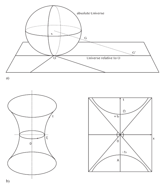
Figure 5.1: De Sitter and Beltrami Castelnuovo Representation: a) de Sitter: The hyperbolic hyperboloid after the application of Wick rotation to S4; b) The P4 Beltrami-Castelnuovo Representation.

Another overturning is obtained in the relationship between cosmology and QM interpretation. We sketched above that the absence of the observer in cosmology generates very peculiar interpretative issues, which concern physical laws, boundary conditions and nucleation. On the other hand, beyond the shortage of the current interpretations, here one finds also the possibility that it could be the same quantum cosmology to suggest a new class of interpretative strategies. This is currently an active research field, which is for example connected to scenarios of eternal inflation [29]. In the framework of Projective Holography, the constrains on the pre-space and on the localization time scale (the chronon) and, in addition, the assumption of the validity of Born Rule in the Archaic Universe, univocally select structure and evolution of the Universe and enables the extension of this approach to particles seen as ”Little Bangs”.

6 Conclusions. Holographies in comparison

Starting from the Lagrangian of a homogeneous and isotropic Universe, a relation between the HH cosmological wave function and a quantum oscillator which works with imaginary time has been derived. This permitted to return again to the problem of the physical meaning of the HH solution and of the centrality of de Sitter Universe in theoretical physics and in contemporary cosmology [57].

In fact, starting from its original proposal [1], the HH wave function received a lot of criticisms. Among such criticisms, the most significant seems to concern the causual relationship between an Euclidean state having imaginary time (without classical space-time) and a Lorentzian metric having real time [58-60].

This kind of questions are present also in the Gamow-Vilenkin-like approach [61, 60], which is founded on the tunnelling mechanism. In that case, the problem is the definition of the barrier. On the other hand, this second big class of models benefited from hypotheses and analogies with quantum field theory, particle physics and black hole physics [62-67].

Thus, it seems that, in its original proposal, the HH wave function cannot escape the general fate of wave functions in quantum mechanics, that is, from the year 1927 wave functions are only a formalism questing a physical interpretation. Another requirement, which is even stronger because of the unicity of the analysed system, is the elevation of the boundary conditions to the level of physical law. The proposal that we suggest in the present work is founded on the cosmological implications of de Sitter relativity and on Projective Holography [35, 68].

One recalls that in de Sitter Universe the cosmological constant is no more a free parameter. It is instead structurally fixed through the introduction of a global curvature which does not depend on gravitational fields. One indeed assumes the hypersphere S4 as being a geometric form of the quantum vacuum, which is, in turn, considered as universal information reservoir or, in more physical terms, as being populated only by virtual processes (imaginary time). This toy model of quantum vacuum has been labelled “Archaic Universe” because its relationship with observables is not chronological. It is logical instead. In fact, the relationship between S4 and the standard post big bang scenario, which works with real time and concerns an accelerated expansion of the Universe, is obtained through Wick rotation and Beltrami-Castelnuovo projection on a plane which is tangential to the hypersphere P4. One notices that every group P4 “inherits” from S4 the same event horizion, and so defines an equal substrate for all the observers. Hence, it completely realizes Weyl’s cosmological principle without contradictions with the quantum realm [69]. Here De Sitter’s eternal is only the hypersphere S4, while the quantities which work with real time and refer to observables are attributed to P4. There are neither physical singularities (but only apparent ones due to the event horizon) nor contradiction (forcing) in the transition between the two different geometries. We argue that the most natural framework for the quantum oscillator (12) should be the surface of S4. Due to time absence, this surface acts as a kind of non local membrane. One among the coordinates of S4 has the role of an archaic precursor of time and, due to the critical temperature (24), it starts to nucleate. In other words, the virtual population starts to show itself in terms of real matter. We argue that this should be the physical essence of the “big bang” and it seems that this kind of description is not too much distant from a traditional description. In traditional relativistic terms, one can say that the hypersphere represents a global boundary condition concerning a big bang with an “isotropic singularity”. This is exactly what is requested by the Wheeler - de Witt equation. The price to pay - which here seems to be favourable - is a different interpretation of the cosmological wave function in terms of product of the wave functions of the nucleated particles. In a oversimplified case, one considers non-symmetrized wave functions, despite one can argue that the nucleated entities are strongly correlated within a non-local framework. This is an “event-based” interpretation, which unifies cosmology and microphysics and is connected with the popular “timeless” approaches, see [18, 30, 70] and references within.

Generally speaking, every physical theory is realized through a formal structure and an interpretation. The interpretation drives the meaning of the formalism and ratifies the “licit” mathematical manipulations. In particular, it specifies the relationship between theory and observations and experiments. Here, the “event-based” approach represents an extension of the standard QM, based on a time scale for the localization. The meaning of the chronon must not be considered as being a “minimum time”. Instead, one considers the chronon as being a time scale compatible with the localization of baryon objects, that is, a kind of classical radius analogous to Bohr’s classical radius of the electron. This is what one expects in a HH semi-classical approach which is very distant from the Planck scale of quantum gravity. We also cite an interesting relation between the two different scales [30, 55], which could be further analysed in future works.

In the framework of de Sitter relativity one finds de Sitter cosmological horizon [30, 68, 71, 72]. The chronological distance from every generic “here”, “now” is a fundamental constant of Nature, $t_{0},$ which is invariant in cosmic time, where $ct_{0}\approx 10^{28}cm$ being $c$ the speed of light [30]. One assumes that the localization of an R process is associate with the formation of a de Sitter micro-horizon centred in $O$ with a radius $c\theta_{0}\approx 10^{-13}$cm, where $O$ is generally delocalized in agreement with the wave function which is entering/outing from the process [30]. The constant $\theta_{0}$ is independent of cosmic time [30]. Thus, also the ratio $\frac{t_{0}}{\theta_{0}}\approx 10^{41}$ results independent of cosmic time [30]. This ratio expresses the number of distinct time localizations which are accessible by the R process within de Sitter cosmological horizon [30]. Basically, $t_{0}$ represents the portion of straight timeline where an observer located in the horizon’s centre positions the R process, while the duration of the R process is order $\theta_{0}.$ Thus, the portion of straight timeline is split in about $10^{41}$ different “cells”. Each cell can stay in one among twt different states: “on” or “off”. The time localization of a single R process corresponds to a situation in which all the cells are “off” with a sole exception of a particular cell which is “on”. Configurations having more that a sole cell which is “on” correspond to the localization various different R process on the same straight timeline. If one assumes that every cell is independent, one has a total of $\left(2^{10}\right)^{41}$ different configurations. Hence, the locational information which is associate with the localization of $0,1,2,...,10^{41}$ R processes amounts to $10^{41}$ bits, the binary logarithm of the number of configurations. This is a kind of information which is codified on the time axis within de Sitter horizon of the observer. The R processes are indeed real interactions among real particles. During such interactions an amount of action of order of the Planck constant $h$ is exchanged. Then, in terms of phase space, the emerging of one among such processes is equivalent to make “on” an elementary cell having a volume of order $h^{3}$. The number of cells which have been made “on” in the phase space of a particular macroscopic physical system is an estimation of the volume that such a system takes up in the same phase space. In other words, it is an estimation of the entropy of the system. Thus, one argues that the information on the localization of the R processes should be connected to the entropy through the uncertainty principle. Thus, it seems natural that one asks if Bekenstein bound on entropy [45] can be applied, in some way, to the two mentioned horizons. Assuming that the information on the time localization of R processes

$$I\equiv\frac{t_{0}}{\theta_{0}}=10^{41}\,bits$$ (41)

is connected to the micro-horizon’s area

$$A=\left(c\theta_{0}\right)^{2}\approx 10^{-26}\,cm^{2},$$ (42)

then, from the holographic relation [30]

$$I=\frac{A}{4l^{2}},$$ (43)

one gets that the spatial extension $l$ of the “cells” which are associated to a bit of informations results to be

$$l\approx 10^{-33}\,cm,$$ (44)

that is the Planck length! On one hand this is an intriguing, remarkable issue. On the other hand it cannot be a coincidence that the Planck scale appears in this way, i.e. as a consequence of the holographic relation (43) combined with the “two horizons” hypothesis and with the finite behavior of the information $I.$ In addition, as both $I$ and $t_{0}$ are connected with the cosmological constant $\Lambda$ through the relation

$$\Lambda=\frac{4}{3t_{0}^{2}},$$ (45)

Eq. (43) substantially defines the Planck length in function of the cosmological constant. In other words, one gets a global-local relation, which is exactly what one expects from a vacuum theory interpreted in terms of information universal reservoir. In this paper, we referred to the connection between the oscillator’s frequency and the cosmological constant. From the above discussion, one can reasonably argue that the holographic conjecture should be a property of the two time-like horizons: the cosmological horizon ($t_{0}$) and the “particle-like” horizon ($\theta_{0}$). This holographic conjecture cannot be generalized to other physical systems (with the exclusion of black holes, because black holes have their proper event horizon). The information associate with the time localization of a physical event (R process) has finite behavior. The same happens for its spatial localization. This is because an observer sees the extension of a transition in Beltrami time as having a lower bound due to the “particle-like” horizon and a higher bound due to the cosmological horizon. This suggests an interesting interpretation of the cosmological constant in terms of “index of spreading information”. In addition, the old matter on the nature of the cosmological constant in terms of geometry vs physics here is bypassed by the Milne-like interpretation. On one hand, in S4 $\Lambda$ appears as a purely geometric ingredient, pertinent to the structure of de Sitter space. On the other hand, in P4 , after the nucleation process and the conversion from information to matter, it is both licit and necessary interpreting the cosmological constant in terms of fields and particles, in particular concerning the open issues on Higgs field and Dark Matter [73 - 77]. The analysis in this paper is limited to a semi-classical approach. Instead, the process of nucleation should imply the emergence of both space and time from a web of elementary events. This is a research field which strongly involves quantum field theory, particle physics and the “universal” role of Higgs field . These issues could be the object of future works of the authors.

We also recall that, after some purely quantum mechanical approach, in the recent literature there are also models of emergent space-time founded on non-locality [78 - 80]. In the scenario analysed in this paper, non-locality means that the Universe’s wave function could nucleate events which are strongly correlated under a drastic, but plausible, symmetrization hypothesis. The mathematical behaviors connected to the maximum symmetry of de Sitter space always fascinated and fascinate theorists, who, in the meanwhile, proposed cosmological and particle physics models [35]. A relevant matter is the development of a consistent quantum field theory in de Sitter space-time. In this framework, the most important problem concerns the stability of de Sitter vacuum and the topological classifications of its decays [81 - 83]. In our opinion, Projective Holography can introduce some clarification in the current debate, by enabling a clear distinction between S4 and P4 [84]. In that direction it could be possible a better understanding of the most traditional holographic approaches connected to Maldacena conjecture [85], in particular through the advent of a new centrality of de Sitter space-time with respect to Anti-de Sitter space-time. In fact, one among the most important problems in this research field consists in projecting an hologram from quantum particle living in the infinite future. This strongly obstructed various efforts in order to describe in holographic terms the real space-time. It is possible to analyse this problem in a S4/P4 framework in order to get a brighter formulation, which seems more practicable after the uplifting result in [86] which transformed two Anti-de Sitter spaces having a saddle shape in de Sitter spaces having bowl shape. Finally, for the sake of completeness, we also signal the recent CPT cosmological hypothesis in [87], which arises from the issue that the S4 structure suggests two specular worlds (most likely Anti-de Sitter spaces). De Sitter Projective Holography shows a structure which is naturally holographic, where the 5D pre-space works as a screen and its projections on the tangential plane P4 represent the bulk, i.e. the expression of the real physical world. In Archaic Holography, the localization and delocalization processes seem as complementary world aspects, while the uncertainty principle represents a “door” between two different levels of physical descriptions: from particle physics to cosmology. Both of them are strongly unified in a global-local connection. On the other hand, going beyond that “door” shows to be less dramatic than physicists were thinking in past research works. In addition, this new scenario seems even more understandable that previous classical scenarios. The relations among various physical quantities like cosmological constant, chronons and Planck length are strongly interconnected and, globally, they indicate the finite behavior of information in Nature.

7 Acknowledgements

I. Licata and C. Corda have been supported financially by the Research Institute for Astronomy and Astrophysics of Maragha (RIAAM). The authors thank Maria Vita Licata for checking the English language.

References

- [1] J. B. Hartle and S. W. Hawking, Phys. Rev. D 28, 2960 (1983).
- [2] B. S. DeWitt, Phys. Rev. 160, 1113 (1967).
- [3] L. D. Landau and E. M. Lifshitz, The Classical Theory of Fields, Pergamon ( 1975).
- [4] A. Einstein, Sit. K. Preu. Akad. Wiss. 142, Berlin (1917).
- [5] L. D. Landau and E. M. Lifshitz, Mechanics, Pergamon ( 1976).
- [6] J. A. Frieman, M. S. Turner and D. Huterer, Ann. Rev. Astron. Astrophys. 46, 385- (2008).
- [7] S. Dodelson, Modern Cosmology (4. [print.]. ed.). San Diego: Academic Press (2003).
- [8] J. J. Sakurai, Modern Quantum Mechanics, Pearson Education (2006).
- [9] M. Ali, S. M. Hassan, and V. Husain, Phys. Rev. D 98, 086002 (2018).
- [10] S. W. Hawking and G. F. R. Ellis, The Large Scale Structure of Space-Time, Cambridge University Press (1973).
- [11] R. Geroch and J. B. Hartle , Found. Phys. 16, 533 (1986).
- [12] S. W. Hawking, T. Hertog and H. S. Reall, Phys. Rev. D 62, 043501 (2000).
- [13] S. W. Hawking and T. Hertog, Phys. Rev. D 73, 123527 (2006).
- [14] S. W. Hawking and T. Hertog, JHEP, 2018, 147 (2018).
- [15] A. F. Ali and S. Das, Phys. Lett. B 741, 276 (2015).
- [16] J. B. Hartle, https://arxiv.org/abs/1901.03933.
- [17] C. Rovelli. Phys. Rev. D 42, 2638 (1990).
- [18] I. Licata and L. Chiatti, Symmetry, 11(2), 181 (2019).
- [19] J. J. Halliwell, J. B. Hartle and T. Hertog, Phys. Rev. D 99, 043526 (2019).
- [20] J. B. Hartle and S. W. Hawking, Phys. Rev. D 13, 2188 (1976).
- [21] S. W. Hawking, Pontif. Acad. Sci. Scr. Varia 48, 563 (1982).
- [22] A. Vilenkin, Phys. Lett. B 117, 25 (1982).
- [23] A. Vilenkin, Phys. Rev. D 30, 509 (1984).
- [24] J. L Lehners and N. Turok, Phys. Rev. Lett. 119, 171301 (2017).
- [25] A. Vilenkin and M. Yamada, Phys. Rev. D 98, 066003 (2018).
- [26] S. Coleman, notes taken by Brian Hill during Sidney Coleman’s lectures on Quantum Field Theory (Physics 253), given at Harvard University in Fall semester of the 1986-1987 academic year and recently typeset and edited by Yuan-Sen Ting and Bryan Gin-ge Chen, arXiv:1110.5013v5.
- [27] R. P. Crease and C. C. Mann, The Second Creation: Makers of the Revolution in Twentieth-Century Physics, Rutgers University Press (1996).
- [28] The Philosophy of Cosmology, Edited by K. Chamcham, University of Oxford, J. Silk, University of Oxford, J. D. Barrow, University of Cambridge, S. Saunders, University of Oxford. Cambridge University Press (2017).
- [29] A. Aguirre and M. Tegmark, Phys.Rev. D 84, 105002 (2011).
- [30] Beyond peaceful coexistence: the emergence of space, time and quantum. Ed. by I. Licata; forew. by G. ’t Hooft, London: Imperial college press (2016).
- [31] A. D. Sakharov, Doklady Akad. Nauk S.S.R. 177, 70 (1987).
- [32] B. L.Hu, Int. J. Theor. Phys. 44, 1785 (2005).
- [33] S. Liberati and L. Maccione, Phys. Rev. Lett. 112, 151301 (2014).
- [34] J. B. Hartle, S. W. Hawking, T. Hertog, Phys. Rev. Lett. 100, 201301 (2008).
- [35] I. Licata, L. Chiatti, E. Benedetto, DE Sitter Projective Relativity, State of the Art for Particles, Fields and Cosmology, Springer (2017).
- [36] I. Licata, EJTP 3(10), 211 (2006).
- [37] I. Licata and L. Chiatti, Int. J. Theor. Phys. 48(4), 1003 (2009).
- [38] I. Licata and L. Chiatti, Int. J. Theor. Phys. 49(10), 2379 (2010).
- [39] L. Chiatti, EJTP 9(26), 11 (2012).
- [40] I. Licata, G. Iovane, L. Chiatti, E. Benedetto, F. Tamburini, Phys. Dark Un. 22, 181 (2018).
- [41] A. Garrett Lisi, arXiv:physics/0605068, 2006.
- [42] G. Arcidiacono, Gen. Rel. Grav. 7, 885 (1976).
- [43] G. Arcidiacono, Gen. Rel. Grav. 8, 865 (1977).
- [44] G. C. Wick, Phys. Rev. 96, 1124 (1954).
- [45] J. D. Bekenstein, Phys. Rev. D 23, 287 (1981).
- [46] R. Pourhasan, N. Afshordi, and R. B. Mann, JCAP 04, 005 (2014).
- [47] A. Baracca, D. Bohm, B. J. Hiley, and A. E. G. Stuart, Nuov. Cim. 28B(2), 453 (1975).
- [48] E. Milne, Relativity, Gravitation and World-structure, Clarendon Press (1935).
- [49] Jonathan Maltz and L. Susskind, Phys. Rev. Lett. 118, 101602 (2017).
- [50] Jonathan Maltz, Phys. Rev. D 95, 066006 (2017).
- [51] R. Geroch and J.B. Hartle, Found. Phys. 16, 533 (1986).
- [52] M. K. Parikh and F. Wilczek, Phys. Rev. Lett. 85, 5042 (2000).
- [53] C. Corda, Class. Quantum Grav. 32, 195007 (2015).
- [54] I. Licata, L. Chiatti, Quant. Stud. Math. Found. 4, 181 (2017).
- [55] I. Licata, L. Chiatti, Quanta 4, 10 (2015).
- [56] N. Rosen, Int. Journ. Theor. Phys. 32, 8 (1993).
- [57] U. Moschella, The de Sitter and anti-de Sitter Sightseeing Tour. Séminaire Poincaré 1-12 (2005).
- [58] R. J. Deltete and R. A. Guy, Synthese, 108(2), 185 (1996).
- [59] R. J. Deltete and R. A. Guy, Analysis 57(4), 304 (1997).
- [60] A. Vilenkin, Phys. Rev. D 58, 067301 (1998).
- [61] G. Gamow Z. Phys. 51(3–4), 204 (1928).
- [62] E. B. Gliner, I.G. Dymnikova Sov. Astron. Lett. 1, 93 (1975).
- [63] R. Brout F. Englert E. Gunzig, Ann. Phys. 115(1), 78 (1978).
- [64] D. Atkatz, H. Pagels, Phys. Rev. D 25, 2065 (1982).
- [65] J. R. Gott III, Nature 295, 304 (1982).
- [66] I. G. Dymnikova A. Dobosz, M. L. Fil’chenkov, A. Gromov, Phys. Lett. B 506(3-4), 351 (2001).
- [67] I. G. Dymnikova, Universe 5(5), 111 (2019).
- [68] R. Aldrovandi, J. G. Pereira, Grav. Cosmol. 15, 287 (2009).
- [69] S. E. Rugh, H. Zinkernagel, arXiv:1006.5848v1 (2010).
- [70] D. Fiscaletti, The Timeless Approach. Frontiers Perspective in 21st Century Physics, World Scientific (2016).
- [71] R. Aldrovandi, J. P. Beltran Almeida, J. G. Pereira, Class. Quant. Grav. 24, 1385 (2007).
- [72] L. Chiatti, arXiv:0901.3616v1 (2009).
- [73] C. O’Raifeartaigh, M. O’Keeffe, W. Nahm and S. Mitton, Eur. Phys. J. H 43, 73 (2018).
- [74] F. Jegerlehner, arXiv:1812.03863 [hep-ph] (2018).
- [75] V. G. Gurzadyan, A. Stepanian, Eur. Phys. J. Plus, 134, 98 (2019).
- [76] F. De Martini, J. Phys. Conf. Ser. 880(1), 012026 (2017).
- [77] F. Jegerlehner, Acta Phys. Polon. B 45, 1215 (2014).
- [78] G. Chew and H. Stapp, Found. Physics 18(8), 809 (1988).
- [79] M. Van Raamsdonk, Int. Journ. Mod. Phys. D 19(14), 2429 (2010).
- [80] C. J. Cao, S. M. Carroll, S. Michalakis, Phys. Rev. D 95, 024031 (2017).
- [81] S. Kanno, J. Soda, Int. J. Mod. Phys. D 21, 1250040 (2012).
- [82] K. K. Boddy, S. M. Carroll, J. Pollack, Found. Phys. 46, 702 (2016).
- [83] H. Epstein, U. Moschella, Int. J. Mod. Phys. A 33(34), 1845009 (2018).
- [84] L. Chiatti, arXiv:0902.1393 (2012).
- [85] J. M. Maldacena, Adv. Theor. Math. Phys. 2, 231 (1998).
- [86] X. Dong, E. Silverstein, G. Torroba, J. High Energ. Phys. 2018, 50 (2018).
- [87] L. Boyle, K. Finn and N. Turok, Phys. Rev. Lett. 121, 251301 (2018)