First-order sensitivity of the optimal value in a Markov decision model with respect to deviations in the transition probability function

Abstract

Markov decision models (MDM) used in practical applications are most often less complex than the underlying ‘true’ MDM. The reduction of model complexity is performed for several reasons. However, it is obviously of interest to know what kind of model reduction is reasonable (in regard to the optimal value) and what kind is not. In this article we propose a way how to address this question. We introduce a sort of derivative of the optimal value as a function of the transition probabilities, which can be used to measure the (first-order) sensitivity of the optimal value w.r.t. changes in the transition probabilities. ‘Differentiability’ is obtained for a fairly broad class of MDMs, and the ‘derivative’ is specified explicitly. Our theoretical findings are illustrated by means of optimization problems in inventory control and mathematical finance.

Keywords: Markov decision model; Model reduction; Transition probability function; Optimal value; Functional differentiability; Financial optimization

1 Introduction

Already in the 1990th, Müller [27] pointed out that the impact of the transition probabilities of a Markov decision process (MDP) on the optimal value of a corresponding Markov decision model (MDM) can not be ignored for practical issues. For instance, in most cases the transition probabilities are unknown and have to be estimated by statistical methods. Moreover in many applications the ‘true’ model is replaced by an approximate version of the ‘true’ model or by a variant which is simplified and thus less complex. The result is that in practical applications the optimal (strategy and thus the optimal) value is most often computed on the basis of transition probabilities that differ from the underlying true transition probabilities. Therefore the sensitivity of the optimal value w.r.t. deviations in the transition probabilities is obviously of interest.

Müller [27] showed that under some structural assumptions the optimal value in a discrete-time MDM depends continuously on the transition probabilities, and he established bounds for the approximation error. In the course of this the distance between transition probabilities was measured by means of some suitable probability metrics. Even earlier, Kolonko [20] obtained analogous bounds in a MDM in which the transition probabilities depend on a parameter. Here the distance between transition probabilities was measured by means of the distance between the respective parameters. Error bounds for the expected total reward of discrete-time Markov reward processes were also specified by van Dijk [40] and van Dijk and Puterman [41]. In the latter reference the authors also discussed the case of discrete-time Markov decision processes with countable state and action spaces.

In this article, we focus on the situation where the ‘true’ model is replaced by a less complex version (for a simple example, see Subsection 5.4.3 in the supplementary material). The reduction of model complexity in practical applications is common and performed for several reasons. Apart from computational aspects and the difficulty of considering all relevant factors, one major point is that statistical inference for certain transition probabilities can be costly in terms of both time and money. However, it is obviously of interest to know what kind of model reduction is reasonable and what kind is not. In the following we want to propose a way how to address the latter question.

Our original motivation comes from the field of optimal logistics transportation planning, where ongoing projects like SYNCHRO-NET [38] aim at stochastic decision models based on transition probabilities estimated from historical route information. Due to the lack of historical data for unlikely events, transition probabilities are often modeled in a simplified way. In fact, events with small probabilities are often ignored in the model. However, the impact of these events on the optimal value (here the minimal expected transportation costs) of the corresponding MDM may nevertheless be significant. The identification of unlikely but potentially cost sensitive events is therefore a major challenge. In logistics planning operations engineers have indeed become increasingly interested in comprehensibly quantifying the sensitivity of the optimal value w.r.t. the incorporation of unlikely events into the model. For background see, for instance, [15, 16]. The assessment of rare but risky events takes on greater importance also in other areas of applications; see, for instance, [21, 44] and references cited therein.

By an incorporation of an unlikely event into the model we mean, for instance, that under performance of an action $a$ at some time $n$ a previously impossible transition from one state $x$ to another state $y$ gets now assigned small but strictly positive probability $\varepsilon$. Mathematically this means that the transition probability $P_{n}((x,a),\,\cdot\,)$ is replaced by $(1-\varepsilon)P_{n}((x,a),\,\bullet\,)+\varepsilon Q_{n}((x,a),\,\bullet\,)$ with $Q_{n}((x,a),\,\bullet\,):=\delta_{y}[\,\bullet\,]$, where $\delta_{y}$ is the Dirac measure at $y$. More generally one could consider a change of the whole transition function (the family of all transition probabilities) $\boldsymbol{P}$ to $(1-\varepsilon)\boldsymbol{P}+\varepsilon\boldsymbol{Q}$ with $\varepsilon>0$ small. For operations engineers it is here interesting to know how this change affects the optimal value, ${\cal V}_{0}(\boldsymbol{P})$. If the effect is minor, then an incorporation can be seen as superfluous, at least from a pragmatic point of view. If on the other hand the effect is significant, then the engineer should consider the option to extend the model and to make an effort to get access to statistical data for the extended model.

At this point it is worth mentioning that a change of the transition function from $\boldsymbol{P}$ to $(1-\varepsilon)\boldsymbol{P}+\varepsilon\boldsymbol{Q}$ with $\varepsilon>0$ small can also have a different interpretation than an incorporation of an (unlikely) new event. It could also be associated with an incorporation of an (unlikely) divergence from the normal transition rules. See Subsection 4.5 for an example.

In this article, we will introduce an approach for quantifying the effect of changing the transition function from $\boldsymbol{P}$ to $(1-\varepsilon)\boldsymbol{P}+\varepsilon\boldsymbol{Q}$, with $\varepsilon>0$ small, on the optimal value ${\cal V}_{0}(\boldsymbol{P})$ of the MDM. In view of $(1-\varepsilon)\boldsymbol{P}+\varepsilon\boldsymbol{Q}=\boldsymbol{P}+\varepsilon(\boldsymbol{Q}-\boldsymbol{P})$, we feel that it is reasonable to quantify the effect by a sort of derivative of the value functional ${\cal V}_{0}$ at $\boldsymbol{P}$ evaluated at direction $\boldsymbol{Q}-\boldsymbol{P}$. To some extent the ‘derivative’ $\dot{\cal V}_{0;\boldsymbol{P}}(\boldsymbol{Q}-\boldsymbol{P})$ specifies the first-order sensitivity of ${\cal V}_{0}(\boldsymbol{P})$ w.r.t. a change of $\boldsymbol{P}$ as above. Take into account that

$${\cal V}_{0}(\boldsymbol{P}+\varepsilon(\boldsymbol{Q}-\boldsymbol{P}))-{\cal V}_{0}(\boldsymbol{P})\,\approx\,\varepsilon\cdot\dot{\cal V}_{0;\boldsymbol{P}}(\boldsymbol{Q}-\boldsymbol{P})\qquad\mbox{for $\varepsilon>0$ small}.$$ (1)

To be able to compare the first-order sensitivity for (infinitely) many different $\boldsymbol{Q}$, it is favourable to know that the approximation in (1) is uniform in $\boldsymbol{Q}\in{\cal K}$ for preferably large sets ${\cal K}$ of transition functions. Moreover, it is not always possible to specify the relevant $\boldsymbol{Q}$ exactly. For that reason it would be also good to have robustness (i.e. some sort of continuity) of $\dot{\cal V}_{0;\boldsymbol{P}}(\boldsymbol{Q}-\boldsymbol{P})$ in $\boldsymbol{Q}$. These two things induced us to focus on a variant of tangential ${\cal S}$-differentiability as introduced by Sebastião e Silva [36] and Averbukh and Smolyanov [1] (here ${\cal S}$ is a family of sets ${\cal K}$ of transition functions). In Section 3 we present a result on ‘${\cal S}$-differentiability’ of ${\cal V}_{0}$ for the family ${\cal S}$ of all relatively compact sets of admissible transition functions and a reasonably broad class of MDMs, where we measure the distance between transition functions by means of metrics based on probability metrics as in [27].

The ‘derivative’ $\dot{\cal V}_{0;\boldsymbol{P}}(\boldsymbol{Q}-\boldsymbol{P})$ of the optimal value functional ${\cal V}_{0}$ at $\boldsymbol{P}$ quantifies the effect of a change from $\boldsymbol{P}$ to $(1-\varepsilon)\boldsymbol{P}+\varepsilon\boldsymbol{Q}$, with $\varepsilon>0$ small, assuming that after the change the strategy $\pi$ (tuple of the underlying decision rules) is chosen such that it optimizes the target value ${\cal V}_{0}^{\pi}(\boldsymbol{P}^{\prime})$ (e.g. expected total costs or rewards) in $\pi$ under the new transition function $\boldsymbol{P}^{\prime}:=(1-\varepsilon)\boldsymbol{P}+\varepsilon\boldsymbol{Q}$. On the other hand, practitioners are also interested in quantifying the impact of a change of $\boldsymbol{P}$ when the optimal strategy (under $\boldsymbol{P}$) is kept after the change. Such a quantification would somehow answers the question: How much different does a strategy derived in a simplified MDM perform in a more complex (more realistic) variant of the MDM? Since the ‘derivative’ $\dot{\cal V}_{0;\boldsymbol{P}}^{\pi}(\boldsymbol{Q}-\boldsymbol{P})$ of the functional ${\cal V}_{0}^{\pi}$ under a fixed strategy $\pi$ turns out to be a building stone for the derivative $\dot{\cal V}_{0;\boldsymbol{P}}(\boldsymbol{Q}-\boldsymbol{P})$ of the optimal value functional ${\cal V}_{0}$ at $\boldsymbol{P}$, our elaborations cover both situations anyway. For fixed strategy $\pi$ we obtain ‘${\cal S}$-differentiability’ of ${\cal V}_{0}^{\pi}$ even for the broader family ${\cal S}$ of all bounded sets of admissible transition functions.

The ‘derivative’ which we propose to regard as a measure for the first-order sensitivity will formally be introduced in Definition 3.9. This definition is applicable to quite general finite time horizon MDMs and might look somewhat cumbersome at first glance. However, in the special case of a finite state space and finite action spaces, a situation one faces in many practical applications, the proposed ‘differentiability’ boils down to a rather intuitive concept. This will be explained in Section 5 of the supplementary material with a minimum of notation and terminology. In Section 5 of the supplementary material we will also reformulate a backward iteration scheme for the computation of the ‘derivative’ (which can be deduced from our main result, Theorem 3.14) in the discrete case, and we will discuss an example.

In Section 2 we formally introduce quite general MDMs in the fashion of the standard monographs [2, 12, 13, 30]. Since it is important to have an elaborate notation in order to formulate our main result, we are very precise in Section 2. As a result, this section is a little longer compared to the respective sections in other articles on MDMs. In Section 3 we carefully introduce our notion of ‘differentiability’ and state our main result concerning the computation of the ‘derivative’ of the value functional.

In Section 4 we will apply the results of Section 3 to assess the impact of one or more than one unlikely but substantial shock in the dynamics of an asset on the solution of a terminal wealth problem in a (simple) financial market model free of shocks. This example somehow motivates the general set-up chosen in Sections 2–3. All results of this article are proven in Sections 7–9 of the supplementary material. For the convenience of the reader we recall in Section 10 of the supplementary material a result on the existence of optimal strategies in general MDMs. Section 11 of the supplementary material contains an auxiliary topological result.

2 Formal definition of Markov decision model

Let $E$ be a non-empty set equipped with a $\sigma$-algebra ${\cal E}$, referred to as state space. Let $N\in\mathbb{N}$ be a fixed finite time horizon (or planning horizon) in discrete time. For each point of time $n=0,\ldots,N-1$ and each state $x\in E$, let $A_{n}(x)$ be a non-empty set. The elements of $A_{n}(x)$ will be seen as the admissible actions (or controls) at time $n$ in state $x$. For each $n=0,\ldots,N-1$, let

$$A_{n}:=\bigcup_{x\in E}A_{n}(x)\quad\mbox{ and }\quad D_{n}:=\big{\{}(x,a)\in E\times A_{n}:\,a\in A_{n}(x)\big{\}}.$$

The elements of $A_{n}$ can be seen as the actions that may basically be selected at time $n$ whereas the elements of $D_{n}$ are the possible state-action combinations at time $n$. For our subsequent analysis, we equip $A_{n}$ with a $\sigma$-algebra ${\cal A}_{n}$, and let ${\cal D}_{n}:=({\cal E}\otimes{\cal A}_{n})\cap D_{n}$ be the trace of the product $\sigma$-algebra ${\cal E}\otimes{\cal A}_{n}$ in $D_{n}$. Recall that a map $P_{n}:D_{n}\times{\cal E}\rightarrow[0,1]$ is said to be a probability kernel (or Markov kernel) from $(D_{n},{\cal D}_{n})$ to $(E,{\cal E})$ if $P_{n}(\,\cdot\,,B)$ is a $({\cal D}_{n},{\cal B}([0,1]))$-measurable map for any $B\in{\cal E}$, and $P_{n}((x,a),\,\bullet\,)\in{\cal M}_{1}(E)$ for any $(x,a)\in D_{n}$. Here ${\cal M}_{1}(E)$ is the set of all probability measures on $(E,{\cal E})$.

2.1 Markov decision process

In this subsection, we will give a formal definition of an $E$-valued (discrete-time) Markov decision process (MDP) associated with a given initial state, a given transition function and a given strategy. By definition a (Markov decision) transition (probability) function is an $N$-tuple

$$\boldsymbol{P}=(P_{0},\ldots,P_{N-1})$$

whose $n$-th entry $P_{n}$ is a probability kernel from $(D_{n},{\cal D}_{n})$ to $(E,{\cal E})$. In this context $P_{n}$ will be referred to as one-step transition (probability) kernel at time $n$ (or from time $n$ to $n+1$) and the probability measure $P_{n}((x,a),\,\bullet\,)$ is referred to as one-step transition probability at time $n$ (or from time $n$ to $n+1$) given state $x$ and action $a$. We denote by ${\cal P}$ the set of all transition functions.

We will assume that the actions are performed by a so-called $N$-stage strategy (or $N$-stage policy). An ($N$-stage) strategy is an $N$-tuple

$$\pi=(f_{0},\ldots,f_{N-1})$$

of decision rules at times $n=0,\ldots,N-1$, where a decision rule at time $n$ is an $({\cal E},{\cal A}_{n})$-measurable map $f_{n}:E\rightarrow A_{n}$ satisfying $f_{n}(x)\in A_{n}(x)$ for all $x\in E$. Note that a decision rule at time $n$ is (deterministic and) ‘Markovian’ since it only depends on the current state and is independent of previous states and actions. We denote by $\mathbb{F}_{n}$ the set of all decision rules at time $n$, and assume that $\mathbb{F}_{n}$ is non-empty. Hence a strategy is an element of the set $\mathbb{F}_{0}\times\cdots\times\mathbb{F}_{N-1}$, and this set can be seen as the set of all strategies. Moreover, we fix for any $n=0,\ldots,N-1$ some $F_{n}\subseteq\mathbb{F}_{n}$ which can be seen as the set of all admissible decision rules at time $n$. In particular, the set $\Pi:=F_{0}\times\cdots\times F_{N-1}$ can be seen as the set of all admissible strategies.

For any transition function $\boldsymbol{P}=(P_{n})_{n=0}^{N-1}\in{\cal P}$, strategy $\pi=(f_{n})_{n=0}^{N-1}\in\Pi$, and time point $n\in\{0,\ldots,N-1\}$, we can derive from $P_{n}$ a probability kernel $P_{n}^{\pi}$ from $(E,{\cal E})$ to $(E,{\cal E})$ through

$$P_{n}^{\pi}(x,B):=P_{n}\big{(}(x,f_{n}(x)),B\big{)},\qquad x\in E,\,B\in{\cal E}.$$ (2)

The probability measure $P_{n}^{\pi}(x,\,\bullet\,)$ can be seen as the one-step transition probability at time $n$ given state $x$ when the transitions and actions are governed by $\boldsymbol{P}$ and $\pi$, respectively.

Now, consider the measurable space

$$(\Omega,{\cal F}):=(E^{N+1},{\cal E}^{\otimes(N+1)}).$$

For any $x_{0}\in E$, $\boldsymbol{P}=(P_{n})_{n=0}^{N-1}\in{\cal P}$, and $\pi\in\Pi$ define the probability measure

$$\mathbb{P}^{x_{0},\boldsymbol{P};\pi}:=\delta_{x_{0}}\otimes P_{0}^{\pi}\otimes\cdots\otimes P_{N-1}^{\pi}$$ (3)

on $(\Omega,{\cal F})$, where $x_{0}$ should be seen as the initial state of the MDP to be constructed. The right-hand side of (3) is the usual product of the probability measure $\delta_{x_{0}}$ and the kernels $P_{0}^{\pi},\ldots,P_{N-1}^{\pi}$; for details see display (6) in Section 6 of the supplementary material. Moreover let $\boldsymbol{X}=(X_{0},\ldots,X_{N})$ be the identity on $\Omega$, i.e.

$$X_{n}(x_{0},\ldots,x_{N}):=x_{n},\qquad(x_{0},\ldots,x_{N})\in E^{N+1},\,n=0,\ldots,N.$$ (4)

Note that, for any $x_{0}\in E$, $\boldsymbol{P}=(P_{n})_{n=0}^{N-1}\in{\cal P}$, and $\pi\in\Pi$, the map $\boldsymbol{X}$ can be regarded as an $(E^{N+1},{\cal E}^{\otimes(N+1)})$-valued random variable on the probability space $(\Omega,{\cal F},\mathbb{P}^{x_{0},\boldsymbol{P};\pi})$ with distribution $\delta_{x_{0}}\otimes P_{0}^{\pi}\otimes\cdots\otimes P_{N-1}^{\pi}$.

It follows from Lemma 6.1 in the supplementary material) that for any $x_{0},\widetilde{x}_{0},\break x_{1},\ldots,x_{n}\in E$, $\boldsymbol{P}=(P_{n})_{n=0}^{N-1}\in{\cal P}$, $\pi=(f_{n})_{n=0}^{N-1}\in\Pi$, and $n=1,\ldots,N-1$

1. $\mathbb{P}^{x_{0},\boldsymbol{P};\pi}[X_{0}\in\,\bullet\,]=\delta_{x_{0}}[\,\bullet\,]$,

2. $\mathbb{P}^{x_{0},\boldsymbol{P};\pi}[X_{1}\in\,\bullet\,\|X_{0}=\widetilde{x}_{0}]=P_{0}\big{(}(x_{0},f_{0}(x_{0})),\,\bullet\,\big{)}$,

3. $\mathbb{P}^{x_{0},\boldsymbol{P};\pi}[X_{n+1}\in\,\bullet\,\|(X_{0},X_{1},\ldots,X_{n})=(\widetilde{x}_{0},x_{1},\ldots,x_{n})]=P_{n}\big{(}(x_{n},f_{n}(x_{n})),\,\bullet\,\big{)}$,

4. $\mathbb{P}^{x_{0},\boldsymbol{P};\pi}[X_{n+1}\in\,\bullet\,\|X_{n}=x_{n}]=P_{n}\big{(}(x_{n},f_{n}(x_{n})),\,\bullet\,\big{)}$.

The formulation of (ii)–(iv) is somewhat sloppy, because in general a (regular version of the) factorized conditional distribution of $X$ given $Y$ under $\mathbb{P}^{x_{0},\boldsymbol{P};\pi}$ (evaluated at a fixed set $B\in{\cal E}$) is only $\mathbb{P}_{Y}^{x_{0},\boldsymbol{P};\pi}$-a.s. unique. So assertion (iv) in fact means that the probability kernel $P_{n}((\,\cdot\,,f_{n}(\,\cdot\,)),\,\bullet\,)$ provides a (regular version of the) factorized conditional distribution of $X_{n+1}$ given $X_{n}$ under $\mathbb{P}^{x_{0},\boldsymbol{P};\pi}$, and analogously for (ii) and (iii). Note that the factorized conditional distribution in part (ii) is constant w.r.t. $\widetilde{x}_{0}\in E$. Assertions (iii) and (iv) together imply that the temporal evolution of $X_{n}$ is Markovian. This justifies the following terminology.

Definition 2.1 (MDP)

Under law $\mathbb{P}^{x_{0},\boldsymbol{P};\pi}$ the random variable $\boldsymbol{X}=(X_{0},\ldots,X_{N})$ is called (discrete-time) Markov decision process (MDP) associated with initial state $x_{0}\in E$, transition function $\boldsymbol{P}\in{\cal P}$ and strategy $\pi\in\Pi$.

2.2 Markov decision model and value function

Maintain the notation and terminology introduced in Subsection 2.1. In this subsection, we will first define a (discrete-time) Markov decision model (MDM) and introduce subsequently the corresponding value function. The latter will be derived from a reward maximization problem. Fix $\boldsymbol{P}\in{\cal P}$, and let for each point of time $n=0,\ldots,N-1$

$$r_{n}:D_{n}\longrightarrow\mathbb{R}$$

be a $({\cal D}_{n},{\cal B}(\mathbb{R}))$-measurable map, referred to as one-stage reward function. Here $r_{n}(x,a)$ specifies the one-stage reward when action $a$ is taken at time $n$ in state $x$. Let

$$r_{N}:E\longrightarrow\mathbb{R}$$

be an $({\cal E},{\cal B}(\mathbb{R}))$-measurable map, referred to as terminal reward function. The value $r_{N}(x)$ specifies the reward of being in state $x$ at terminal time $N$.

Denote by $\boldsymbol{A}$ the family of all sets $A_{n}(x)$, $n=0,\ldots,N-1$, $x\in E$, and set $\boldsymbol{r}:=(r_{n})_{n=0}^{N}$. Moreover let $\boldsymbol{X}$ be defined as in (4) and recall Definition 2.1. Then we define our MDM as follows.

Definition 2.2 (MDM)

The quintuple $(\boldsymbol{X},\boldsymbol{A},\boldsymbol{P},\Pi,\boldsymbol{r})$ is called (discrete-time) Markov decision model (MDM) associated with the family of action spaces $\boldsymbol{A}$, transition function $\boldsymbol{P}\in{\cal P}$, set of admissible strategies $\Pi$, and reward functions $\boldsymbol{r}$.

In the sequel we will always assume that a MDM $(\boldsymbol{X},\boldsymbol{A},\boldsymbol{P},\Pi,\boldsymbol{r})$ satisfies the following Assumption (A). In Subsection 3.1 we will discuss some conditions on the MDM under which Assumption (A) holds. We will use $\mathbb{E}_{n,x_{n}}^{x_{0},\boldsymbol{P};\pi}$ to denote the expectation w.r.t. the factorized conditional distribution $\mathbb{P}^{x_{0},\boldsymbol{P};\pi}[\,\bullet\,\|X_{n}=x_{n}]$. For $n=0$, we clearly have $\mathbb{P}^{x_{0},\boldsymbol{P};\pi}[\,\bullet\,\|X_{0}=x_{0}]=\mathbb{P}^{x_{0},\boldsymbol{P};\pi}[\,\bullet\,]$ for every $x_{0}\in E$; see Lemma 6.1 in the supplementary material. In what follows we use the convention that the sum over the empty set is zero.

Assumption (A):  $\sup_{\pi=(f_{n})_{n=0}^{N-1}\in\Pi}\mathbb{E}_{n,x_{n}}^{x_{0},\boldsymbol{P};\pi}[\,\sum_{k=n}^{N-1}|r_{k}(X_{k},f_{k}(X_{k}))|+|r_{N}(X_{N})|\,]<\infty$ for any $x_{n}\in E$ and $n=0,\ldots,N$.

Under Assumption (A) we may define in a MDM $(\boldsymbol{X},\boldsymbol{A},\boldsymbol{P},\Pi,\boldsymbol{r})$ for any $\pi=(f_{n})_{n=0}^{N-1}\in\Pi$ and $n=0,\ldots,N$ a map $V_{n}^{\boldsymbol{P};\pi}:E\rightarrow\mathbb{R}$ through

$$V_{n}^{\boldsymbol{P};\pi}(x_{n}):=\mathbb{E}_{n,x_{n}}^{x_{0},\boldsymbol{P};\pi}\Big{[}\sum_{k=n}^{N-1}r_{k}(X_{k},f_{k}(X_{k}))+r_{N}(X_{N})\Big{]}.$$ (5)

As a factorized conditional expectation this map is $({\cal E},{\cal B}(\mathbb{R}))$-measurable (for any $\pi\in\Pi$ and $n=0,\ldots,N$). Note that for $n=1,\ldots,N$ the right-hand side of (5) does not depend on $x_{0}$; see Lemma 6.2 in the supplementary material. Therefore the map $V_{n}^{\boldsymbol{P};\pi}(\cdot)$ need not be equipped with an index $x_{0}$.

The value $V_{n}^{\boldsymbol{P};\pi}(x_{n})$ specifies the expected total reward from time $n$ to $N$ of $\boldsymbol{X}$ under $\mathbb{P}^{x_{0},\boldsymbol{P};\pi}$ when strategy $\pi$ is used and $\boldsymbol{X}$ is in state $x_{n}$ at time $n$. It is natural to ask for those strategies $\pi\in\Pi$ for which the expected total reward from time $0$ to $N$ is maximal for all initial states $x_{0}\in E$. This results in the following optimization problem:

$$V_{0}^{\boldsymbol{P};\pi}(x_{0})\longrightarrow\max\ \mbox{(in $\pi\in\Pi$)\,!}$$ (6)

If a solution $\pi^{\boldsymbol{P}}$ to the optimization problem (6) (in the sense of Definition 2.4 ahead) exists, then the corresponding maximal expected total reward is given by the so-called value function (at time $0$).

Definition 2.3 (Value function)

For a MDM $(\boldsymbol{X},\boldsymbol{A},\boldsymbol{P},\Pi,\boldsymbol{r})$ the value function at time $n\in\{0,\ldots,N\}$ is the map $V_{n}^{\boldsymbol{P}}:E\rightarrow\mathbb{R}$ defined by

$$V_{n}^{\boldsymbol{P}}(x_{n}):=\sup_{\pi\in\Pi}V_{n}^{\boldsymbol{P};\pi}(x_{n}).$$ (7)

Note that the value function $V_{n}^{\boldsymbol{P}}$ is well defined due to Assumption (A) but not necessarily $({\cal E},{\cal B}(\mathbb{R}))$-measurable. The measurability holds true, for example, if the sets $F_{n},\ldots,F_{N-1}$ are at most countable or if conditions (a)–(c) of Theorem 10.3 in the supplementary material) are satisfied; see also Remark 10.4(i) in the supplementary material.

Definition 2.4 (Optimal strategy)

In a MDM $(\boldsymbol{X},\boldsymbol{A},\boldsymbol{P},\Pi,\boldsymbol{r})$ a strategy $\pi^{\boldsymbol{P}}\in\Pi$ is called optimal w.r.t. $\boldsymbol{P}$ if

$$V_{0}^{\boldsymbol{P};\pi^{\boldsymbol{P}}}(x_{0})=V_{0}^{\boldsymbol{P}}(x_{0})\quad\mbox{for all }x_{0}\in E.$$ (8)

In this case $V_{0}^{\boldsymbol{P};\pi^{\boldsymbol{P}}}(x_{0})$ is called optimal value (function), and we denote by $\Pi(\boldsymbol{P})$ the set of all optimal strategies w.r.t. $\boldsymbol{P}$. Further, for any given $\delta>0$, a strategy $\pi^{\boldsymbol{P};\delta}\in\Pi$ is called $\delta$-optimal w.r.t. $\boldsymbol{P}$ in a MDM $(\boldsymbol{X},\boldsymbol{A},\boldsymbol{P},\Pi,\boldsymbol{r})$ if

$$V_{0}^{\boldsymbol{P}}(x_{0})-\delta\leq V_{0}^{\boldsymbol{P};\pi^{\boldsymbol{P};\delta}}(x_{0})\quad\mbox{for all }x_{0}\in E,$$ (9)

and we denote by $\Pi(\boldsymbol{P};\delta)$ the set of all $\delta$-optimal strategies w.r.t. $\boldsymbol{P}$.

Note that condition (8) requires that $\pi^{\boldsymbol{P}}\in\Pi$ is an optimal strategy for all possible initial states $x_{0}\in E$. Though, in some situations it might be sufficient to ensure that $\pi^{\boldsymbol{P}}\in\Pi$ is an optimal strategy only for some fixed initial state $x_{0}$. For a brief discussion of the existence and computation of optimal strategies, see Section 10 of the supplementary material.

Remark 2.5

(i) In practice, the choice of an action can possibly be based on historical observations of states and actions. In particular one could relinquish the Markov property of the decision rules and allow them to depend also on previous states and actions. Then one might hope that the corresponding (deterministic) history-dependent strategies improve the optimal value of a MDM $(\boldsymbol{X},\boldsymbol{A},\boldsymbol{P},\Pi,\boldsymbol{r})$. However, it is known that the optimal value of a MDM $(\boldsymbol{X},\boldsymbol{A},\boldsymbol{P},\Pi,\boldsymbol{r})$ can not be enhanced by considering history-dependent strategies; see, e.g., Theorem 18.4 in [13] or Theorem 4.5.1 in [30].

(ii) Instead of considering the reward maximization problem (6) one could as well be interested in minimizing expected total costs over the time horizon $N$. In this case, one can maintain the previous notation and terminology when regarding the functions $r_{n}$ and $r_{N}$ as the one-stage costs and the terminal costs, respectively. The only thing one has to do is to replace “$\sup$” by “$\inf$” in the representation (7) of the value function. Accordingly, a strategy $\pi^{\boldsymbol{P};\delta}\in\Pi$ will be $\delta$-optimal for a given $\delta>0$ if in condition (9) “$-\delta$” and “$\leq$” are replaced by “$+\delta$” and “$\geq$”. $\Diamond$

3 ‘Differentiability’ in $\boldsymbol{P}$ of the optimal value

In this section, we show that the value function of a MDM, regarded as a real-valued functional on a set of transition functions, is ‘differentiable’ in a certain sense. The notion of ‘differentiability’ we use for functionals that are defined on a set of admissible transition functions will be introduced in Subsection 3.4. The motivation of our notion of ‘differentiability’ was discussed subsequent to (1). Before defining ‘differentiability’ in a precise way, we will explain in Subsections 3.2–3.3 how we measure the distance between transition functions. In Subsections 3.5–3.6 we will specify the ‘Hadamard derivative’ of the value function. At first, however, we will discuss in Subsection 3.1 some conditions under which Assumption (A) holds true. Throughout this section, $\boldsymbol{A}$, $\Pi$, and $\boldsymbol{r}$ are fixed.

3.1 Bounding functions

Recall from Section 2 that ${\cal P}$ stands for the set of all transition functions, i.e. of all $N$-tuples $\boldsymbol{P}=(P_{n})_{n=0}^{N-1}$ of probability kernels $P_{n}$ from $(D_{n},{\cal D}_{n})$ to $(E,{\cal E})$. Let $\psi:E\rightarrow\mathbb{R}_{\geq 1}$ be an $({\cal E},{\cal B}(\mathbb{R}_{\geq 1}))$-measurable map, referred to as gauge function, where $\mathbb{R}_{\geq 1}:=[1,\infty)$. Denote by $\mathbb{M}(E)$ the set of all $({\cal E},{\cal B}(\mathbb{R}))$-measurable maps $h\in\mathbb{R}^{E}$, and let $\mathbb{M}_{\psi}(E)$ be the set of all $h\in\mathbb{M}(E)$ satisfying $\|h\|_{\psi}:=\sup_{x\in E}|h(x)|/\psi(x)<\infty$. The following definition is adapted from [2, 27, 43]. Conditions (a)–(c) of this definition are sufficient for the well-definiteness of $V_{n}^{\boldsymbol{P};\pi}$ (and $V_{n}^{\boldsymbol{P}}$); see Lemma 3.2 ahead.

Definition 3.1 (Bounding function)

Let ${\cal P}^{\prime}\subseteq{\cal P}$. A gauge function $\psi:E\to\mathbb{R}_{\geq 1}$ is called a bounding function for the family of MDMs $\{(\boldsymbol{X},\boldsymbol{A},\boldsymbol{P},\Pi,\boldsymbol{r}):\boldsymbol{P}\in{\cal P}^{\prime}\}$ if there exist finite constants $K_{1},K_{2},K_{3}>0$ such that the following conditions hold for any $n=0,\ldots,N-1$ and $\boldsymbol{P}=(P_{n})_{n=0}^{N-1}\in{\cal P}^{\prime}$.

1. $|r_{n}(x,a)|\leq K_{1}\psi(x)$ for all $(x,a)\in D_{n}$.

2. $|r_{N}(x)|\leq K_{2}\psi(x)$ for all $x\in E$.

3. $\int_{E}\psi(y)\,P_{n}\big{(}(x,a),dy\big{)}\leq K_{3}\psi(x)$ for all $(x,a)\in D_{n}$.

If ${\cal P}^{\prime}=\{\boldsymbol{P}\}$ for some $\boldsymbol{P}\in{\cal P}$, then $\psi$ is called a bounding function for the MDM $(\boldsymbol{X},\boldsymbol{A},\boldsymbol{P},\Pi,\boldsymbol{r})$.

Note that the conditions in Definition 3.1 do not depend on the set $\Pi$. That is, the terminology bounding function is independent of the set of all (admissible) strategies. Also note that conditions (a) and (b) can be satisfied by unbounded reward functions.

The following lemma, whose proof can be found in Subsection 7.1 of the supplementary material, ensures that Assumption (A) is satisfied when the underlying MDM possesses a bounding function.

Lemma 3.2

Let ${\cal P}^{\prime}\subseteq{\cal P}$. If the family of MDMs $\{(\boldsymbol{X},\boldsymbol{A},\boldsymbol{P},\Pi,\boldsymbol{r}):\boldsymbol{P}\in{\cal P}^{\prime}\}$ possesses a bounding function $\psi$, then Assumption (A) is satisfied for any $\boldsymbol{P}\in{\cal P}^{\prime}$. Moreover, the expectation in Assumption (A) is even uniformly bounded w.r.t. $\boldsymbol{P}\in{\cal P}^{\prime}$, and $V_{n}^{\boldsymbol{P};\pi}(\cdot)$ is contained in $\mathbb{M}_{\psi}(E)$ for any $\boldsymbol{P}\in{\cal P}^{\prime}$, $\pi\in\Pi$, and $n=0,\ldots,N$.

3.2 Metric on set of probability measures

In Subsection 3.4 we will work with a (semi-) metric (on a set of transition functions) to be defined in (11) below. As it is common in the theory of probability metrics (see, e.g., p. 10 ff in [31]), we allow the distance between two probability measures and the distance between two transition functions to be infinite. That is, we adapt the axioms of a (semi-) metric but we allow a (semi-) metric to take values in $\overline{\mathbb{R}}_{\geq 0}:=\mathbb{R}_{\geq 0}\cup\{\infty\}$ rather than only in $\mathbb{R}_{\geq 0}:=[0,\infty)$.

Let $\psi$ be any gauge function, and denote by ${\cal M}_{1}^{\psi}(E)$ the set of all $\mu\in{\cal M}_{1}(E)$ for which $\int_{E}\psi\,d\mu<\infty$. Note that the integral $\int_{E}h\,d\mu$ exists and is finite for any $h\in\mathbb{M}_{\psi}(E)$ and $\mu\in{\cal M}_{1}^{\psi}(E)$. For any fixed $\mathbb{M}\subseteq\mathbb{M}_{\psi}(E)$, the distance between two probability measures $\mu,\nu\in{\cal M}_{1}^{\psi}(E)$ can be measured by

$$d_{\mathbb{M}}(\mu,\nu):=\sup_{h\in\mathbb{M}}\Big{|}\int_{E}h\,d\mu-\int_{E}h\,d\nu\Big{|}.$$ (10)

Note that (10) indeed defines a map $d_{\mathbb{M}}:{\cal M}_{1}^{\psi}(E)\times{\cal M}_{1}^{\psi}(E)\rightarrow\overline{\mathbb{R}}_{+}$ which is symmetric and fulfills the triangle inequality, i.e. $d_{\mathbb{M}}$ provides a semi-metric. If $\mathbb{M}$ separates points in ${\cal M}_{1}^{\psi}(E)$ (i.e. if any two $\mu,\nu\in{\cal M}_{1}^{\psi}(E)$ coincide when $\int_{E}h\,d\mu=\int_{E}h\,d\nu$ for all $h\in\mathbb{M}$), then $d_{\mathbb{M}}$ is even a metric. It is sometimes called integral probability metric or probability metric with a $\zeta$-structure; see [28, 45]. In some situations the (semi-) metric $d_{\mathbb{M}}$ (with $\mathbb{M}$ fixed) can be represented by the right-hand side of (10) with $\mathbb{M}$ replaced by a different subset $\mathbb{M}^{\prime}$ of $\mathbb{M}_{\psi}(E)$. Each such set $\mathbb{M}^{\prime}$ is said to be a generator of $d_{\mathbb{M}}$. The largest generator of $d_{\mathbb{M}}$ is called the maximal generator of $d_{\mathbb{M}}$ and denoted by $\overline{\mathbb{M}}$. That is, $\overline{\mathbb{M}}$ is defined to be the set of all $h\in\mathbb{M}_{\psi}(E)$ for which $|\int_{E}h\,d\mu-\int_{E}h\,d\nu|\leq d_{\mathbb{M}}(\mu,\nu)$ for all $\mu,\nu\in{\cal M}_{1}^{\psi}(E)$.

We now give some examples for the distance $d_{\mathbb{M}}$. The metrics in the first four examples were already mentioned in [27, 28]. In the last three examples $d_{\mathbb{M}}$ metricizes the $\psi$-weak topology. The latter is defined to be the coarsest topology on ${\cal M}_{1}^{\psi}(E)$ for which all mappings $\mu\mapsto\int_{E}h\,d\mu$, $h\in\mathbb{C}_{\psi}(E)$, are continuous. Here $\mathbb{C}_{\psi}(E)$ is the set of all continuous functions in $\mathbb{M}_{\psi}(E)$. If specifically $\psi\equiv 1$, then ${\cal M}_{1}^{\psi}(E)={\cal M}_{1}(E)$ and the $\psi$-weak topology is nothing but the classical weak topology. In Section 2 in [23] one can find characterizations of those subsets of ${\cal M}_{1}^{\psi}(E)$ on which the relative $\psi$-weak topology coincides with the relative weak topology.

Example 3.3

Let $\psi:\equiv 1$ and $\mathbb{M}:=\mathbb{M}_{\mathrm{\scriptsize{TV}}}$, where $\mathbb{M}_{\mathrm{\scriptsize{TV}}}:=\{\mathbbm{1}_{B}:B\in{\cal E}\}\subseteq\mathbb{M}_{\psi}(E)$. Then $d_{\mathbb{M}}$ equals the total variation metric $d_{\mathrm{\scriptsize{TV}}}(\mu,\nu):=\sup_{B\in{\cal E}}|\mu[B]-\nu[B]|$. The set $\mathbb{M}_{\mathrm{\scriptsize{TV}}}$ clearly separates points in ${\cal M}_{1}^{\psi}(E)={\cal M}_{1}(E)$. The maximal generator of $d_{\mathrm{\scriptsize{TV}}}$ is the set $\overline{\mathbb{M}}_{\mathrm{\scriptsize{TV}}}$ of all $h\in\mathbb{M}(E)$ with ${\mathrm{s}p}(h):=\sup_{x\in E}h(x)-\inf_{x\in E}h(x)\leq 1$; see Theorem 5.4 in [28]. $\Diamond$

Example 3.4

For $E=\mathbb{R}$, let $\psi:\equiv 1$ and $\mathbb{M}:=\mathbb{M}_{\mathrm{\scriptsize{Kolm}}}$, where $\mathbb{M}_{\mathrm{\scriptsize{Kolm}}}:=\{\mathbbm{1}_{(-\infty,t]}:t\in\mathbb{R}\}\subseteq\mathbb{M}_{\psi}(\mathbb{R})$. Then $d_{\mathbb{M}}$ equals the Kolmogorov metric $d_{\mathrm{\scriptsize{Kolm}}}(\mu,\nu):=\sup_{t\in\mathbb{R}}|F_{\mu}(t)-F_{\nu}(t)|$, where $F_{\mu}$ and $F_{\nu}$ refer to the distribution functions of $\mu$ and $\nu$, respectively. The set $\mathbb{M}_{\mathrm{\scriptsize{Kolm}}}$ clearly separates points in ${\cal M}_{1}^{\psi}(\mathbb{R})={\cal M}_{1}(\mathbb{R})$. The maximal generator of $d_{\mathrm{\scriptsize{Kolm}}}$ is the set $\overline{\mathbb{M}}_{\mathrm{\scriptsize{Kolm}}}$ of all $h\in\mathbb{R}^{\mathbb{R}}$ with $\mathbb{V}(h)\leq 1$, where $\mathbb{V}(h)$ denotes the total variation of $h$; see Theorem 5.2 in [28]. $\Diamond$

Example 3.5

Assume that $(E,d_{E})$ is a metric space and let ${\cal E}:={\cal B}(E)$. Let $\psi:\equiv 1$ and $\mathbb{M}:=\mathbb{M}_{\mathrm{\scriptsize{BL}}}$, where $\mathbb{M}_{\mathrm{\scriptsize{BL}}}:=\{h\in\mathbb{R}^{E}:\|h\|_{\mathrm{\scriptsize{BL}}}\leq 1\}\subseteq\mathbb{M}_{\psi}(E)$ with $\|h\|_{\mathrm{\scriptsize{BL}}}:=\max\{\|h\|_{\infty},\,\|h\|_{\mathrm{\scriptsize{Lip}}}\}$ for $\|h\|_{\infty}:=\sup_{x\in E}|h(x)|$ and $\|h\|_{\mathrm{\scriptsize{Lip}}}:=\sup_{x,y\in E:\,x\neq y}|h(x)-\break h(y)|/d_{E}(x,y)$. Then $d_{\mathbb{M}}$ is nothing but the bounded Lipschitz metric $d_{\mathrm{\scriptsize{BL}}}$. The set $\mathbb{M}_{\mathrm{\scriptsize{BL}}}$ separates points in ${\cal M}_{1}^{\psi}(E)={\cal M}_{1}(E)$; see Lemma 9.3.2 in [8]. Moreover it is known (see, e.g., Theorem 11.3.3 in [8]) that if $E$ is separable then $d_{\mathrm{\scriptsize{BL}}}$ metricizes the weak topology on ${\cal M}_{1}^{\psi}(E)={\cal M}_{1}(E)$. $\Diamond$

Example 3.6

Assume that $(E,d_{E})$ is a metric space and let ${\cal E}:={\cal B}(E)$. For some fixed $x^{\prime}\in E$, let $\psi(x):=1+d_{E}(x,x^{\prime})$ and $\mathbb{M}:=\mathbb{M}_{\mathrm{\scriptsize{Kant}}}$, where $\mathbb{M}_{\mathrm{K}ant}:=\{h\in\mathbb{R}^{E}:\|h\|_{\mathrm{\scriptsize{Lip}}}\leq 1\}\subseteq\mathbb{M}_{\psi}(E)$ with $\|h\|_{\mathrm{\scriptsize{Lip}}}$ as in Example 3.5. Then $d_{\mathbb{M}}$ is nothing but the Kantorovich metric $d_{\mathrm{\scriptsize{Kant}}}$. The set $\mathbb{M}_{\mathrm{\scriptsize{Kant}}}$ separates points in ${\cal M}_{1}^{\psi}(E)$, because $\mathbb{M}_{\mathrm{\scriptsize{BL}}}$ ($\subseteq\mathbb{M}_{\mathrm{\scriptsize{Kant}}}$) does. It is known (see, e.g., Theorem 7.12 in [42]) that if $E$ is complete and separable then $d_{\mathrm{\scriptsize{Kant}}}$ metricizes the $\psi$-weak topology on ${\cal M}_{1}^{\psi}(E)$.

Recall from [39] that for $E=\mathbb{R}$ the $L^{1}$-Wasserstein metric $d_{{\mathrm{\scriptsize{Wass}}}_{1}}(\mu,\nu):=\int_{-\infty}^{\infty}|F_{\mu}(t)-F_{\nu}(t)|\,dt$ coincides with the Kantorovich metric. In this case the $\psi$-weak topology is also referred to as $L^{1}$-weak topology. Note that the $L^{1}$-Wasserstein metric is a conventional metric for measuring the distance between probability distributions; see, for instance, [7, 18, 39] for the general concept and [4, 19, 22, 24] for recent applications. $\Diamond$

Although the Kantorovich metric is a popular and well established metric, for the application in Section 4 we will need the following generalization from $\alpha=1$ to $\alpha\in(0,1]$.

Example 3.7

Assume that $(E,d_{E})$ is a metric space and let ${\cal E}:={\cal B}(E)$. For some fixed $x^{\prime}\in E$ and $\alpha\in(0,1]$, let $\psi(x):=1+d_{E}(x,x^{\prime})^{\alpha}$ and $\mathbb{M}:=\mathbb{M}_{\mathrm{\scriptsize{H\ddot{o}l}},\alpha}$, where $\mathbb{M}_{\mathrm{\scriptsize{H\ddot{o}l}},\alpha}:=\{h\in\mathbb{R}^{E}:\|h\|_{\mathrm{\scriptsize{H\ddot{o}l}},\alpha}\leq 1\}\subseteq\mathbb{M}_{\psi}(E)$ with $\|h\|_{\mathrm{\scriptsize{H\ddot{o}l}},\alpha}:=\sup_{x,y\in E:\,x\neq y}|h(x)\break-h(y)|/d_{E}(x,y)^{\alpha}$. The set $\mathbb{M}_{\mathrm{\scriptsize{H\ddot{o}l}},\alpha}$ separates points in ${\cal M}_{1}^{\psi}(E)$ (this follows with similar arguments as in the proof of Lemma 9.3.2 in [8]). Then $d_{\mathbb{M}}$ provides a metric on ${\cal M}_{1}^{\psi}(E)$ which we denote by $d_{\mathrm{\scriptsize{H\ddot{o}l}},\alpha}$ and refer to as Hölder-$\alpha$ metric. Especially when dealing with risk averse utility functions (as, e.g., in Section 4) this metric can be beneficial. Lemma 11.1 in Section 11 of the supplementary material shows that if $E$ is complete and separable then $d_{\mathrm{\scriptsize{H\ddot{o}l}},\alpha}$ metricizes the $\psi$-weak topology on ${\cal M}_{1}^{\psi}(E)$. $\Diamond$

3.3 Metric on set of transition functions

Maintain the notation from Subsection 3.2. Let us denote by $\overline{\cal P}_{\psi}$ the set of all transition functions $\boldsymbol{P}=(P_{n})_{n=0}^{N-1}\in{\cal P}$ satisfying $\int_{E}\psi(y)\,P_{n}((x,a),dy)<\infty$ for all $(x,a)\in D_{n}$ and $n=0,\ldots,N-1$. That is, $\overline{\cal P}_{\psi}$ consists of those transition functions $\boldsymbol{P}=(P_{n})_{n=0}^{N-1}\in{\cal P}$ with $P_{n}((x,a),\,\bullet\,)\in{\cal M}_{1}^{\psi}(E)$ for all $(x,a)\in D_{n}$ and $n=0,\ldots,N-1$. Hence, for the elements $\boldsymbol{P}=(P_{n})_{n=0}^{N-1}$ of $\overline{\cal P}_{\psi}$ all integrals of the shape $\int_{E}h(y)\,P_{n}((x,a),dy)$, $h\in\mathbb{M}_{\psi}(E)$, $(x,a)\in D_{n}$, $n=0,\ldots,N-1$, exist and are finite. In particular, for two transition functions $\boldsymbol{P}=(P_{n})_{n=0}^{N-1}$ and $\boldsymbol{Q}=(Q_{n})_{n=0}^{N-1}$ from $\overline{\cal P}_{\psi}$ the distance $d_{\mathbb{M}}(P_{n}((x,a),\,\bullet\,),Q_{n}((x,a),\,\bullet\,))$ is well defined for all $(x,a)\in D_{n}$ and $n=0,\ldots,N-1$ (recall that $\mathbb{M}\subseteq\mathbb{M}_{\psi}(E)$). So we can define the distance between two transition functions $\boldsymbol{P}=(P_{n})_{n=0}^{N-1}$ and $\boldsymbol{Q}=(Q_{n})_{n=0}^{N-1}$ from $\overline{\cal P}_{\psi}$ by

$$d_{\infty,\mathbb{M}}^{\phi}(\boldsymbol{P},\boldsymbol{Q}):=\max_{n=0,\ldots,N-1}\sup_{(x,a)\in D_{n}}\,\frac{1}{\phi(x)}\cdot d_{\mathbb{M}}\Big{(}P_{n}\big{(}(x,a),\,\bullet\,\big{)},Q_{n}\big{(}(x,a),\,\bullet\,\big{)}\Big{)}$$ (11)

for another gauge function $\phi:E\to\mathbb{R}_{\geq 1}$. Note that (11) defines a semi-metric $d_{\infty,\mathbb{M}}^{\phi}:\overline{\cal P}_{\psi}\times\overline{\cal P}_{\psi}\rightarrow\overline{\mathbb{R}}_{\geq 0}$ on $\overline{\cal P}_{\psi}$ which is even a metric if $\mathbb{M}$ separates points in ${\cal M}_{1}^{\psi}(E)$.

Maybe apart from the factor $1/\phi(x)$, the definition of $d_{\infty,\mathbb{M}}^{\phi}(\boldsymbol{P},\boldsymbol{Q})$ in (11) is quite natural and in line with the definition of a distance introduced by Müller [27, p. 880]. In [27], Müller considers time-homogeneous MDMs, so that the transition kernels do not depend on $n$. He fixed a state $x$ and took the supremum only over all admissible actions $a$ in state $x$. That is, for any $x\in E$ he defined the distance between $P((x,\,\cdot\,),\,\bullet\,)$ and $Q((x,\,\cdot\,),\,\bullet\,)$ by $\sup_{a\in A(x)}d_{\mathbb{M}}(P((x,a),\,\bullet\,),Q((x,a),\,\bullet\,))$. To obtain a reasonable distance between $P_{n}$ and $Q_{n}$ it is however natural to take the supremum of the distance between $P_{n}((x,\,\cdot\,),\,\bullet\,)$ and $Q_{n}((x,\,\cdot\,),\,\bullet\,)$ uniformly over $a$ and over $x$.

The factor $1/\phi(x)$ in (11) causes that the (semi-) metric $d_{\infty,\mathbb{M}}^{\phi}$ is less strict compared to the (semi-) metric $d_{\infty,\mathbb{M}}^{1}$ which is defined as in (11) with $\phi:\equiv 1$. For a motivation of considering the factor $1/\phi(x)$, see part (iii) of Remark 3.10 and the discussion afterwards.

3.4 Definition of ‘differentiability’

Let $\psi$ be any gauge function, and fix some ${\cal P}_{\psi}\subseteq\overline{\cal P}_{\psi}$ being closed under mixtures (i.e. $(1-\varepsilon)\boldsymbol{P}+\varepsilon\boldsymbol{Q}\in{\cal P}_{\psi}$ for any $\boldsymbol{P},\boldsymbol{Q}\in{\cal P}_{\psi}$, $\varepsilon\in(0,1)$). The set ${\cal P}_{\psi}$ will be equipped with the distance $d_{\infty,\mathbb{M}}^{\phi}$ introduced in (11). In Definition 3.9 below we will introduce a reasonable notion of ‘differentiability’ for an arbitrary functional ${\cal V}:{\cal P}_{\psi}\rightarrow L$ taking values in a normed vector space $(L,\|\cdot\|_{L})$. It is related to the general functional analytic concept of (tangential) ${\cal S}$-differentiability introduced by Sebastião e Silva [36] and Averbukh and Smolyanov [1]; see also [9, 11, 37] for applications. However, ${\cal P}_{\psi}$ is not a vector space. This implies that Definition 3.9 differs from the classical notion of (tangential) ${\cal S}$-differentiability. For that reason we will use inverted commas and write ‘${\cal S}$-differentiability’ instead of ${\cal S}$-differentiability. Due to the missing vector space structure, we in particular need to allow the tangent space to depend on the point $\boldsymbol{P}\in{\cal P}_{\psi}$ at which ${\cal V}$ is differentiated. The role of the ‘tangent space’ will be played by the set

$${\cal P}_{\psi}^{\boldsymbol{P};\pm}:=\{\boldsymbol{Q}-\boldsymbol{P}:\,\boldsymbol{Q}\in{\cal P}_{\psi}\}$$

whose elements $\boldsymbol{Q}-\boldsymbol{P}:=(Q_{0}-P_{0},\ldots,Q_{N-1}-P_{N-1})$ can be seen as signed transition functions. In Definition 3.9 we will employ the following terminology.

Definition 3.8

Let $\mathbb{M}\subseteq\mathbb{M}_{\psi}(E)$, $\phi$ be another gauge function, and fix $\boldsymbol{P}\in{\cal P}_{\psi}$. A map ${\cal W}:{\cal P}_{\psi}^{\boldsymbol{P};\pm}\rightarrow L$ is said to be $(\mathbb{M},\phi)$-continuous if the mapping $\boldsymbol{Q}\mapsto{\cal W}(\boldsymbol{Q}-\boldsymbol{P})$ from ${\cal P}_{\psi}$ to $L$ is $(d_{\infty,\mathbb{M}}^{\phi},\|\cdot\|_{L})$-continuous.

For the following definition it is important to note that $\boldsymbol{P}+\varepsilon(\boldsymbol{Q}-\boldsymbol{P})$ lies in ${\cal P}_{\psi}$ for any $\boldsymbol{P},\boldsymbol{Q}\in{\cal P}_{\psi}$ and $\varepsilon\in(0,1]$.

Definition 3.9 (‘${\cal S}$-differentiability’)

Let $\mathbb{M}\subseteq\mathbb{M}_{\psi}(E)$, $\phi$ be another gauge function, and fix $\boldsymbol{P}\in{\cal P}_{\psi}$. Moreover let ${\cal S}$ be a system of subsets of ${\cal P}_{\psi}$. A map ${\cal V}:{\cal P}_{\psi}\rightarrow L$ is said to be ‘${\cal S}$-differentiable’ at $\boldsymbol{P}$ w.r.t. $(\mathbb{M},\phi)$ if there exists an $(\mathbb{M},\phi)$-continuous map $\dot{\cal V}_{\boldsymbol{P}}:{\cal P}_{\psi}^{\boldsymbol{P};\pm}\rightarrow L$ such that

$$\lim_{m\to\infty}\Big{\|}\frac{{\cal V}(\boldsymbol{P}+\varepsilon_{m}(\boldsymbol{Q}-\boldsymbol{P}))-{\cal V}(\boldsymbol{P})}{\varepsilon_{m}}-\dot{\cal V}_{\boldsymbol{P}}(\boldsymbol{Q}-\boldsymbol{P})\Big{\|}_{L}=0\quad\mbox{uniformly in $\boldsymbol{Q}\in{\cal K}$}$$ (12)

for every ${\cal K}\in{\cal S}$ and every sequence $(\varepsilon_{m})\in(0,1]^{\mathbb{N}}$ with $\varepsilon_{m}\to 0$. In this case, $\dot{\cal V}_{\boldsymbol{P}}$ is called ‘${\cal S}$-derivative’ of ${\cal V}$ at $\boldsymbol{P}$ w.r.t. $(\mathbb{M},\phi)$.

Note that in Definition 3.9 the derivative is not required to be linear (in fact the derivative is not even defined on a vector space). This is another point where Definition 3.9 differs from the functional analytic definition of (tangential) ${\cal S}$-differentiability. However, non-linear derivatives are common in the field of mathematical optimization; see, for instance, [32, 37].

Remark 3.10

(i) At least in the case $L=\mathbb{R}$, the ‘${\cal S}$-derivative’ $\dot{\cal V}_{\boldsymbol{P}}$ evaluated at $\boldsymbol{Q}-\boldsymbol{P}$, i.e. $\dot{\cal V}_{\boldsymbol{P}}(\boldsymbol{Q}-\boldsymbol{P})$, can be seen as a measure for the first-order sensitivity of the functional ${\cal V}:{\cal P}_{\psi}\to\mathbb{R}$ w.r.t. a change of the argument from $\boldsymbol{P}$ to $(1-\varepsilon)\boldsymbol{P}+\varepsilon\boldsymbol{Q}$, with $\varepsilon>0$ small, for some given transition function $\boldsymbol{Q}$.

(ii) The prefix ‘${\cal S}$-’ in Definition 3.9 provides the following information. Since the convergence in (12) is required to be uniform in $\boldsymbol{Q}\in{\cal K}$, the values of the first-order sensitivities $\dot{\cal V}_{\boldsymbol{P}}(\boldsymbol{Q}-\boldsymbol{P})$, $\boldsymbol{Q}\in{\cal K}$, can be compared with each other with clear conscience for any fixed ${\cal K}\in{\cal S}$. It is therefore favorable if the sets in ${\cal S}$ are large. However, the larger the sets in ${\cal S}$, the stricter the condition of ‘${\cal S}$-differentiability’.

(iii) The subset $\mathbb{M}$ ($\subseteq\mathbb{M}_{\psi}(E)$) and the gauge function $\phi$ tell us in a way how ‘robust’ the ‘${\cal S}$-derivative’ $\dot{\cal V}_{\boldsymbol{P}}$ is w.r.t. changes in $\boldsymbol{Q}$: The smaller the set $\mathbb{M}$ and the ‘steeper’ the gauge function $\phi$, the less strict the metric $d_{\infty,\mathbb{M}}^{\phi}(\boldsymbol{P},\boldsymbol{Q})$ (given by (11)), and therefore the more robust $\dot{\cal V}_{\boldsymbol{P}}(\boldsymbol{Q}-\boldsymbol{P})$ in $\boldsymbol{Q}$. It is thus favorable if the set $\mathbb{M}$ is small and the gauge function $\phi$ is ‘steep’. However, the smaller $\mathbb{M}$ and the ‘steeper’ $\phi$, the stricter the condition of ‘${\cal S}$-differentiability’. More precisely, if $\mathbb{M}_{1}\subseteq\mathbb{M}_{2}$ and $\phi_{1}\geq\phi_{2}$ then ‘${\cal S}$-differentiability’ w.r.t. $(\mathbb{M}_{1},\phi_{1})$ implies ‘${\cal S}$-differentiability’ w.r.t. $(\mathbb{M}_{2},\phi_{2})$. Also note that in general the choice of ${\cal S}$ in Definition 3.9 is not influenced by the choice of the pair $(\mathbb{M},\phi)$, and vice versa. $\Diamond$

In the general framework of our main result (Theorem 3.14) we can not choose $\phi$ ‘steeper’ than the gauge function $\psi$ which plays the role of a bounding function there. Indeed, the proof of $(\mathbb{M},\psi)$-continuity of the map $\dot{\cal V}_{\boldsymbol{P}}:{\cal P}_{\psi}^{\boldsymbol{P};\pm}\rightarrow\mathbb{R}$ in Theorem 3.14 does not work anymore if $d_{\infty,\mathbb{M}}^{\psi}$ is replaced by $d_{\infty,\mathbb{M}}^{\phi}$ for any gauge function $\phi$ ‘steeper’ than $\psi$. And here it does not matter how exactly ${\cal S}$ is chosen.

In the application in Section 4, the set $\{\boldsymbol{Q}_{\Delta,\tau}:\Delta\in[0,\delta]\}$ should be contained in ${\cal S}$ (for details see Remark 4.8). This set can be shown to be (relatively) compact w.r.t. $d_{\infty,\mathbb{M}}^{\phi}$ for $\phi(x)=\psi(x)$ ($:=1+u_{\alpha}(x)$) but not for any ‘flatter’ gauge function $\phi$. So, in this example, and certainly in many other examples, relatively compact subsets of ${\cal P}_{\psi}$ w.r.t. $d_{\infty,\mathbb{M}}^{\psi}$ should be contained in ${\cal S}$. It is thus often beneficial to know that the value functional is ‘differentiable’ in the sense of part (b) of the following Definition 3.11.

The terminology of Definition 3.11 is motivated by the functional analytic analogues. Bounded and relatively compact sets in the (semi-) metric space $({\cal P}_{\psi},d_{\infty,\mathbb{M}}^{\phi})$ are understood in the conventional way. A set ${\cal K}\subseteq{\cal P}_{\psi}$ is said to be bounded (w.r.t. $d_{\infty,\mathbb{M}}^{\phi}$) if there exist $\boldsymbol{P}^{\prime}\in{\cal P}_{\psi}$ and $\delta>0$ such that $d_{\infty,\mathbb{M}}^{\phi}(\boldsymbol{Q},\boldsymbol{P}^{\prime})\leq\delta$ for every $\boldsymbol{Q}\in{\cal K}$. It is said to be relatively compact (w.r.t. $d_{\infty,\mathbb{M}}^{\phi}$) if for every sequence $(\boldsymbol{Q}_{m})\in{\cal K}^{\mathbb{N}}$ there exists a subsequence $(\boldsymbol{Q}^{\prime}_{m})$ of $(\boldsymbol{Q}_{m})$ such that $d_{\infty,\mathbb{M}}^{\phi}(\boldsymbol{Q}_{m}^{\prime},\boldsymbol{Q})\to 0$ for some $\boldsymbol{Q}\in{\cal P}_{\psi}$. The system of all bounded sets and the system of all relatively compact sets (w.r.t. $d_{\infty,\mathbb{M}}^{\phi}$) are larger the ‘steeper’ the gauge function $\phi$ is.

Definition 3.11

In the setting of Definition 3.9 we refer to ‘${\cal S}$-differentiability’ as

1. ‘Gateaux–Lévy differentiability’ if ${\cal S}={\cal S}_{{\mathrm{f}}}:=\{{\cal K}\subseteq{\cal P}_{\psi}:{\cal K}\mbox{ is finite}\}$.

2. ‘Hadamard differentiability’ if ${\cal S}={\cal S}_{{\mathrm{r}c}}:=\{{\cal K}\subseteq{\cal P}_{\psi}:{\cal K}\mbox{ is relatively compact}\}$.

3. ‘Fréchet differentiability’ if ${\cal S}={\cal S}_{{\mathrm{b}}}:=\{{\cal K}\subseteq{\cal P}_{\psi}:{\cal K}\mbox{ is bounded}\}$.

Clearly, ‘Fréchet differentiability’ (of ${\cal V}$ at $\boldsymbol{P}$ w.r.t. $(\mathbb{M},\phi)$) implies ‘Hadamard differentiability’ which in turn implies ‘Gateaux–Lévy differentiability’, each with the same ‘derivative’.

The last sentence before Definition 3.11 and the second to last sentence in part (iii) of Remark 3.10 together imply that ‘Hadamard (resp. Fréchet) differentiability’ w.r.t. $(\mathbb{M},\phi_{1})$ implies ‘Hadamard (resp. Fréchet) differentiability’ w.r.t. $(\mathbb{M},\phi_{2})$ when $\phi_{1}\geq\phi_{2}$.

The following lemma, whose proof can be found in Subsection 7.2 of the supplementary material, provides an equivalent characterization of ‘Hadamard differentiability’.

Lemma 3.12

Let $\mathbb{M}\subseteq\mathbb{M}_{\psi}(E)$, $\phi$ be another gauge function, ${\cal V}:{\cal P}_{\psi}\rightarrow L$ be any map, and fix $\boldsymbol{P}\in{\cal P}_{\psi}$. Then the following two assertions hold.

(i) If ${\cal V}$ is ‘Hadamard differentiable’ at $\boldsymbol{P}$ w.r.t. $(\mathbb{M},\phi)$ with ‘Hadamard derivative’ $\dot{\cal V}_{\boldsymbol{P}}$, then we have for each triplet $(\boldsymbol{Q},(\boldsymbol{Q}_{m}),(\varepsilon_{m}))\in{\cal P}_{\psi}\times{\cal P}_{\psi}^{\mathbb{N}}\times(0,1]^{\mathbb{N}}$ with $d_{\infty,\mathbb{M}}^{\phi}(\boldsymbol{Q}_{m},\boldsymbol{Q})\to 0$ and $\varepsilon_{m}\to 0$ that

$$\lim_{m\to\infty}\Big{\|}\frac{{\cal V}(\boldsymbol{P}+\varepsilon_{m}(\boldsymbol{Q}_{m}-\boldsymbol{P}))-{\cal V}(\boldsymbol{P})}{\varepsilon_{m}}-\dot{\cal V}_{\boldsymbol{P}}(\boldsymbol{Q}-\boldsymbol{P})\Big{\|}_{L}=0.$$ (13)

(ii) If there exists an $(\mathbb{M},\phi)$-continuous map $\dot{\cal V}_{\boldsymbol{P}}:{\cal P}_{\psi}^{\boldsymbol{P};\pm}\rightarrow L$ such that (13) holds for each triplet $(\boldsymbol{Q},(\boldsymbol{Q}_{m}),(\varepsilon_{m}))\in{\cal P}_{\psi}\times{\cal P}_{\psi}^{\mathbb{N}}\times(0,1]^{\mathbb{N}}$ with $d_{\infty,\mathbb{M}}^{\phi}(\boldsymbol{Q}_{m},\boldsymbol{Q})\to 0$ and $\varepsilon_{m}\to 0$, then ${\cal V}$ is ‘Hadamard differentiable’ at $\boldsymbol{P}$ w.r.t. $(\mathbb{M},\phi)$ with ‘Hadamard derivative’ $\dot{\cal V}_{\boldsymbol{P}}$.

3.5 ‘Differentiability’ of the value functional

Recall that $\boldsymbol{A}$, $\Pi$, and $\boldsymbol{r}$ are fixed, and let $V_{n}^{\boldsymbol{P};\pi}$ and $V_{n}^{\boldsymbol{P}}$ be defined as in (5) and (7), respectively. Moreover let $\psi$ be any gauge function and fix some ${\cal P}_{\psi}\subseteq\overline{\cal P}_{\psi}$ being closed under mixtures.

In view of Lemma 3.2 (with ${\cal P}^{\prime}:=\{\boldsymbol{P}\}$), condition (a) of Theorem 3.14 below ensures that Assumption (A) is satisfied for any $\boldsymbol{P}\in{\cal P}_{\psi}$. Then for any $x_{n}\in E$, $\pi\in\Pi$, and $n=0,\ldots,N$ we may define under condition (a) of Theorem 3.14 functionals ${\cal V}_{n}^{x_{n};\pi}:{\cal P}_{\psi}\rightarrow\mathbb{R}$ and ${\cal V}_{n}^{x_{n}}:{\cal P}_{\psi}\rightarrow\mathbb{R}$ by

$${\cal V}_{n}^{x_{n};\pi}(\boldsymbol{P}):=V_{n}^{\boldsymbol{P};\pi}(x_{n})\quad\mbox{ and }\quad{\cal V}_{n}^{x_{n}}(\boldsymbol{P}):=V_{n}^{\boldsymbol{P}}(x_{n}),$$ (14)

respectively. Note that ${\cal V}_{n}^{x_{n}}(\boldsymbol{P})$ specifies the maximal value for the expected total reward in the MDM (given state $x_{n}$ at time $n$) when the underlying transition function is $\boldsymbol{P}$. By analogy with the name ‘value function’ we refer to ${\cal V}_{n}^{x_{n}}$ as value functional given state $x_{n}$ at time $n$. Part (ii) of Theorem 3.14 provides (under some assumptions) an ‘Hadamard derivative’ of the value functional ${\cal V}_{n}^{x_{n}}$ in the sense of Definition 3.11.

Conditions (b) and (c) of Theorem 3.14 involve the so-called Minkowski (or gauge) functional $\rho_{\mathbb{M}}:\mathbb{M}_{\psi}(E)\rightarrow\overline{\mathbb{R}}_{+}$ (see, e.g., [33, p. 25]) defined by

$$\rho_{\mathbb{M}}(h):=\inf\big{\{}\lambda\in\mathbb{R}_{>0}:\,h/\lambda\in\mathbb{M}\big{\}},$$ (15)

where we use the convention $\inf\emptyset:=\infty$, $\mathbb{M}$ is any subset of $\mathbb{M}_{\psi}(E)$, and we set $\mathbb{R}_{>0}:=(0,\infty)$. We note that Müller [27] also used the Minkowski functional to formulate his assumptions.

Example 3.13

For the sets $\mathbb{M}$ (and the corresponding gauge functions $\psi$) from Examples 3.3–3.7 we have $\rho_{\overline{\mathbb{M}}_{\mathrm{\scriptsize{TV}}}}(h)={\mathrm{s}p}(h)$, $\rho_{\overline{\mathbb{M}}_{\mathrm{\scriptsize{Kolm}}}}(h)=\mathbb{V}(h)$, $\rho_{\mathbb{M}_{\mathrm{\scriptsize{BL}}}}(h)=\|h\|_{\mathrm{B}L}$, $\rho_{\mathbb{M}_{\mathrm{\scriptsize{Kant}}}}(h)=\|h\|_{\mathrm{L}ip}$, and $\rho_{\mathbb{M}_{\mathrm{\scriptsize{H\ddot{o}l}},\alpha}}(h)=\|h\|_{\mathrm{\scriptsize{H\ddot{o}l}},\alpha}$, where as before $\overline{\mathbb{M}}_{\mathrm{\scriptsize{TV}}}$ and $\overline{\mathbb{M}}_{\mathrm{\scriptsize{Kolm}}}$ are used to denote the maximal generator of $d_{\mathrm{\scriptsize{TV}}}$ and $d_{\mathrm{\scriptsize{Kolm}}}$, respectively. The latter three equations are trivial, for the former two equations see [27, p. 880]. $\Diamond$

Recall from Definition 2.4 that for given $\boldsymbol{P}\in{\cal P}_{\psi}$ and $\delta>0$ the sets $\Pi(\boldsymbol{P};\delta)$ and $\Pi(\boldsymbol{P})$ consist of all $\delta$-optimal strategies w.r.t. $\boldsymbol{P}$ and of all optimal strategies w.r.t. $\boldsymbol{P}$, respectively. Generators $\mathbb{M}^{\prime}$ of $d_{\mathbb{M}}$ were introduced subsequent to (10).

Theorem 3.14 (‘Differentiability’ of ${\cal V}_{n}^{x_{n};\pi}$ and ${\cal V}_{n}^{x_{n}}$)

Let $\mathbb{M}\subseteq\mathbb{M}_{\psi}(E)$ and $\mathbb{M}^{\prime}$ be any generator of $d_{\mathbb{M}}$. Fix $\boldsymbol{P}=(P_{n})_{n=0}^{N-1}\in{\cal P}_{\psi}$, and assume that the following three conditions hold.

1. $\psi$ is a bounding function for the MDM $(\boldsymbol{X},\boldsymbol{A},\boldsymbol{Q},\Pi,\boldsymbol{r})$ for any $\boldsymbol{Q}\in{\cal P}_{\psi}$.

2. $\sup_{\pi\in\Pi}\rho_{\mathbb{M}^{\prime}}(V_{n}^{\boldsymbol{P};\pi})<\infty$ for any $n=1,\ldots,N$.

3. $\rho_{\mathbb{M}^{\prime}}(\psi)<\infty$.

Then the following two assertions hold.

1. For any $x_{n}\in E$, $\pi=(f_{n})_{n=0}^{N-1}\in\Pi$, $n=0,\ldots,N$, the map ${\cal V}_{n}^{x_{n};\pi}:{\cal P}_{\psi}\rightarrow\mathbb{R}$ defined by (14) is ‘Fréchet differentiable’ at $\boldsymbol{P}$ w.r.t. $(\mathbb{M},\psi)$ with ‘Fréchet derivative’ $\dot{\cal V}_{n;\boldsymbol{P}}^{x_{n};\pi}:{\cal P}_{\psi}^{\boldsymbol{P};\pm}\rightarrow\mathbb{R}$ given by

   $$\dot{\cal V}_{n;\boldsymbol{P}}^{x_{n};\pi}(\boldsymbol{Q}-\boldsymbol{P})$$

   $$:= \sum_{k=n+1}^{N-1}\sum_{j=n}^{k-1}\int_{E}\cdots\int_{E}r_{k}(y_{k},f_{k}(y_{k}))\,P_{k-1}\big{(}(y_{k-1},f_{k-1}(y_{k-1})),dy_{k}\big{)}$$

   $$\quad\cdots(Q_{j}-P_{j})\big{(}(y_{j},f_{j}(y_{j})),dy_{j+1}\big{)}\cdots P_{n}\big{(}(x_{n},f_{n}(x_{n})),dy_{n+1}\big{)}$$

   $$+\leavevmode\nobreak\ \sum_{j=n}^{N-1}\int_{E}\cdots\int_{E}r_{N}(y_{N})\,P_{N-1}\big{(}(y_{N-1},f_{N-1}(y_{N-1})),dy_{N}\big{)}$$

   $$\quad\cdots(Q_{j}-P_{j})\big{(}(y_{j},f_{j}(y_{j})),dy_{j+1}\big{)}\cdots P_{n}\big{(}(x_{n},f_{n}(x_{n})),dy_{n+1}\big{)}.$$

2. For any $x_{n}\in E$ and $n=0,\ldots,N$, the map ${\cal V}_{n}^{x_{n}}:{\cal P}_{\psi}\rightarrow\mathbb{R}$ defined by (14) is ‘Hadamard differentiable’ at $\boldsymbol{P}$ w.r.t. $(\mathbb{M},\psi)$ with ‘Hadamard derivative’ $\dot{\cal V}_{n;\boldsymbol{P}}^{x_{n}}:{\cal P}_{\psi}^{\boldsymbol{P};\pm}\rightarrow\mathbb{R}$ given by

   $$\dot{\cal V}_{n;\boldsymbol{P}}^{x_{n}}(\boldsymbol{Q}-\boldsymbol{P}):=\lim_{\delta\searrow 0}\,\sup_{\pi\in\Pi(\boldsymbol{P};\delta)}\dot{\cal V}_{n;\boldsymbol{P}}^{x_{n};\pi}(\boldsymbol{Q}-\boldsymbol{P}).$$ (17)

   If the set of optimal strategies $\Pi(\boldsymbol{P})$ is non-empty, then the ‘Hadamard derivative’ admits the representation

   $$\dot{\cal V}_{n;\boldsymbol{P}}^{x_{n}}(\boldsymbol{Q}-\boldsymbol{P})=\sup_{\pi\in\Pi(\boldsymbol{P})}\dot{\cal V}_{n;\boldsymbol{P}}^{x_{n};\pi}(\boldsymbol{Q}-\boldsymbol{P}).$$ (18)

The proof of Theorem 3.14 can be found in Section 8 of the supplementary material. Note that the set $\Pi(\boldsymbol{P};\delta)$ shrinks as $\delta$ decreases. Therefore the right-hand side of (17) is well defined. The supremum in (18) ranges over all optimal strategies w.r.t. $\boldsymbol{P}$. If, for example, the MDM $(\boldsymbol{X},\boldsymbol{A},\boldsymbol{P},\Pi,\boldsymbol{r})$ satisfies conditions (a)–(c) of Theorem 10.3 in the supplementary material, then by part (iii) of this theorem an optimal strategy can be found, i.e. $\Pi(\boldsymbol{P})$ is non-empty. The existence of an optimal strategy is also ensured if the sets $F_{0},\ldots,F_{N-1}$ are finite (a situation one often faces in applications). In the latter case the ‘Hadamard derivative’ $\dot{\cal V}_{n;\boldsymbol{P}}^{x_{n}}(\boldsymbol{Q}-\boldsymbol{P})$ can easily be determined by computing the finitely many values $\dot{\cal V}_{n;\boldsymbol{P}}^{x_{n};\pi}(\boldsymbol{Q}-\boldsymbol{P})$, $\pi\in\Pi(\boldsymbol{P})$, and taking their maximum. The discrete case will be discussed in more detail in Subsection 5.5 of the supplementary material.

If there exists a unique optimal strategy $\pi^{\boldsymbol{P}}\in\Pi$ w.r.t. $\boldsymbol{P}$, then $\Pi(\boldsymbol{P})$ is nothing but the singleton $\{\pi^{\boldsymbol{P}}\}$, and in this case the ‘Hadamard derivative’ $\dot{\cal V}_{0;\boldsymbol{P}}^{x_{0}}$ of the optimal value (functional) ${\cal V}_{0}^{x_{0}}$ at $\boldsymbol{P}$ coincides with $\dot{\cal V}_{0;\boldsymbol{P}}^{x_{0};\pi^{\boldsymbol{P}}}$.

Remark 3.15

(i) The ‘Fréchet differentiability’ in part (i) of Theorem 3.14 holds even uniformly in $\pi\in\Pi$; see Theorem 8.1 in the supplementary material for the precise meaning.

(ii) We do not know if it is possible to replace ‘Hadamard differentiability’ by ‘Fréchet differentiability’ in part (ii) of Theorem 3.14. The following arguments rather cast doubt on this possibility. The proof of part (ii) is based on the decomposition of the value functional ${\cal V}_{n}^{x_{n}}$ in display (73) of the supplementary material and a suitable chain rule, where the decomposition (73) involves the sup-functional $\Psi$ introduced in display (74) of the supplementary material. However, Corollary 1 in [6] (see also Proposition 4.6.5 in [35]) shows that in normed vector spaces sup-functionals are in general not Fréchet differentiable. This could be an indication that ‘Fréchet differentiable’ of the value functional indeed fails. We can not make a reliable statement in this regard.

(iii) Recall that ‘Hadamard (resp. Fréchet) differentiability’ w.r.t. $(\mathbb{M},\psi)$ implies ‘Hadamard (resp. Fréchet) differentiability’ w.r.t. $(\mathbb{M},\phi)$ for any gauge function $\phi\leq\psi$. However, for any such $\phi$ ‘Hadamard (resp. Fréchet) differentiability’ w.r.t. $(\mathbb{M},\phi)$ is less meaningful than w.r.t. $(\mathbb{M},\psi)$. Indeed, when using $d_{\infty,\mathbb{M}}^{\phi}$ with $\phi\leq\psi$ instead of $d_{\infty,\mathbb{M}}^{\psi}$, the sets ${\cal K}$ for whose elements the first-order sensitivities can be compared with each other with clear conscience are smaller and the ‘derivative’ is less robust.

(iv) In the case where we are interested in minimizing expected total costs in the MDM $(\boldsymbol{X},\boldsymbol{A},\boldsymbol{P},\Pi,\boldsymbol{r})$ (see Remark 2.5(ii)), we obtain under the assumptions (and with the same arguments as in the proof of part (ii)) of Theorem 3.14 that the ‘Hadamard derivative’ of the corresponding value functional is given by (17) (resp. (18)) with “$\sup$” replaced by “$\inf$”. $\Diamond$

Remark 3.16

(i) Condition (a) of Theorem 3.14 is in line with the existing literature. In fact, similar conditions as in Definition 3.1 (with ${\cal P}^{\prime}:=\{\boldsymbol{Q}\}$) have been imposed many times before; see, for instance, [2, Definition 2.4.1], [27, Definition 2.4], [30, p. 231 ff], and [43].

(ii) In some situations, condition (a) implies condition (b) in Theorem 3.14. This is the case, for instance, in the following four settings (the involved sets $\mathbb{M}^{\prime}$ were introduced in Examples 3.3–3.7).

1) $\mathbb{M}^{\prime}:=\overline{\mathbb{M}}_{\mathrm{\scriptsize{TV}}}$ and $\psi:\equiv 1$.

2) $\mathbb{M}^{\prime}:=\overline{\mathbb{M}}_{\mathrm{\scriptsize{Kolm}}}$ and $\psi:\equiv 1$, as well as for $n=1,\ldots,N-1$
        - $\int_{\mathbb{R}}V_{n+1}^{\boldsymbol{P};\pi}(y)\,P_{n}((\,\cdot\,,f_{n}(\,\cdot\,)),dy)$, $\pi=(f_{n})_{n=0}^{N-1}\in\Pi$, are increasing,
        - $r_{n}(\,\cdot\,,f_{n}(\,\cdot\,))$, $\pi=(f_{n})_{n=0}^{N-1}\in\Pi$, and $r_{N}(\cdot)$ are increasing.

3) $\mathbb{M}^{\prime}:=\mathbb{M}_{\mathrm{\scriptsize{BL}}}$ and $\psi:\equiv 1$, as well as for $n=1,\ldots,N-1$
        - $\sup_{\pi=(f_{n})_{n=0}^{N-1}\in\Pi}\sup_{x\not=y}d_{\mathrm{\scriptsize{BL}}}(P_{n}((x,f_{n}(x)),\,\bullet\,),P_{n}((y,f_{n}(y)),\,\bullet\,))/d_{E}(x,y)<\infty$,
        - $\sup_{\pi=(f_{n})_{n=0}^{N-1}\in\Pi}\|r_{n}(\,\cdot\,,f_{n}(\,\cdot\,))\|_{\mathrm{\scriptsize{Lip}}}<\infty$ and $\|r_{N}\|_{\mathrm{\scriptsize{Lip}}}<\infty$.

4) $\mathbb{M}^{\prime}:=\mathbb{M}_{\mathrm{\scriptsize{H\ddot{o}l}},\alpha}$ and $\psi(x):=1+d_{E}(x,x^{\prime})^{\alpha}$, as well as for $n=1,\ldots,N-1$
        - $\sup_{\pi=(f_{n})_{n=0}^{N-1}\in\Pi}\sup_{x\not=y}d_{\mathrm{\scriptsize{H\ddot{o}l}},\alpha}(P_{n}((x,f_{n}(x)),\,\bullet\,),P_{n}((y,f_{n}(y)),\,\bullet\,))/d_{E}(x,y)^{\alpha}<\infty$,
        - $\sup_{\pi=(f_{n})_{n=0}^{N-1}\in\Pi}\|r_{n}(\,\cdot\,,f_{n}(\,\cdot\,))\|_{\mathrm{\scriptsize{H\ddot{o}l}},\alpha}<\infty$ and $\|r_{N}\|_{\mathrm{\scriptsize{H\ddot{o}l}},\alpha}<\infty$ for some $x^{\prime}\in E$ and
        $\alpha\in(0,1]$. Recall that $\mathbb{M}_{\mathrm{\scriptsize{H\ddot{o}l}},\alpha}=\mathbb{M}_{\mathrm{\scriptsize{Kant}}}$ for $\alpha=1$.

The proof of (a)$\Rightarrow$(b) relies in setting 1) on Lemma 3.2 (with ${\cal P}^{\prime}:=\{\boldsymbol{P}\}$) and in settings 2)–4) on Lemma 3.2 (with ${\cal P}^{\prime}:=\{\boldsymbol{P}\}$) along with Proposition 10.1 of the supplementary material. The conditions in setting 2) are similar to those in parts (ii)–(iv) of Theorem 2.4.14 in [2], and the conditions in settings 3) and 4) are motivated by the statements in [14, p. 11f].

(iii) In many situations, condition (c) of Theorem 3.14 holds trivially. This is the case, for instance, if $\mathbb{M}^{\prime}\in\{\overline{\mathbb{M}}_{\mathrm{\scriptsize{TV}}},\overline{\mathbb{M}}_{\mathrm{\scriptsize{Kolm}}},\mathbb{M}_{\mathrm{\scriptsize{BL}}}\}$ and $\psi:\equiv 1$, or if $\mathbb{M}^{\prime}:=\mathbb{M}_{\mathrm{\scriptsize{H\ddot{o}l}},\alpha}$ and $\psi(x):=1+d_{E}(x,x^{\prime})^{\alpha}$ for some fixed $x^{\prime}\in E$ and $\alpha\in(0,1]$.

(iv) The conditions (b) and (c) of Theorem 3.14 can also be verified directly in some cases; see, for instance, the proof of Lemma 9.2 in Subsection 9.3.1 of the supplementary material. $\Diamond$

In applications it is not necessarily easy to specify the set $\Pi(\boldsymbol{P})$ of all optimal strategies w.r.t. $\boldsymbol{P}$. While in most cases an optimal strategy can be found with little effort (one can use the Bellman equation; see part (i) of Theorem 10.3 in Section 10 of the supplementary material), it is typically more involved to specify all optimal strategies or to show that the optimal strategy is unique. The following remark may help in some situations; for an application see Subsection 4.4.

Remark 3.17

In some situations it turns out that for every $\boldsymbol{P}\in{\cal P}_{\psi}$ the solution of the optimization problem (6) does not change if $\Pi$ is replaced by a subset $\Pi^{\prime}\subseteq\Pi$ (being independent of $\boldsymbol{P}$). Then in the definition (7) of the value function (at time $0$) the set $\Pi$ can be replaced by the subset $\Pi^{\prime}$, and it follows (under the assumptions of Theorem 3.14) that in the representation (18) of the ‘Hadamard derivative’ $\dot{\cal V}_{0;\boldsymbol{P}}^{x_{0}}$ of ${\cal V}_{0}^{x_{0}}$ at $\boldsymbol{P}$ the set $\Pi(\boldsymbol{P})$ can be replaced by the set $\Pi^{\prime}(\boldsymbol{P})$ of all optimal strategies w.r.t. $\boldsymbol{P}$ from the subset $\Pi^{\prime}$. Of course, in this case it suffices to ensure that conditions (a)–(b) of Theorem 3.14 are satisfied for the subset $\Pi^{\prime}$ instead of $\Pi$. $\Diamond$

3.6 Two alternative representations of $\dot{\cal V}_{n;\boldsymbol{P}}^{x_{n};\pi}$

In this subsection we present two alternative representations (see (19) and (20)) of the ‘Fréchet derivative’ $\dot{\cal V}_{n;\boldsymbol{P}}^{x_{n};\pi}$ in ((i)). The representation (19) will be beneficial for the proof of Theorem 3.14 (see Lemma 8.2 in Subsection 8.1 of the supplementary material) and the representation (20) will be used to derive the ‘Hadamard derivative’ of the optimal value of the terminal wealth problem in (28) below (see the proof of Theorem 4.6 in Subsection 9.3 of the supplementary material).

Remark 3.18 (Representation I)

By rearranging the sums in ((i)), we obtain under the assumptions of Theorem 3.14 that for every fixed $\boldsymbol{P}=(P_{n})_{n=0}^{N-1}\in{\cal P}_{\psi}$ the ‘Fréchet derivative’ $\dot{\cal V}_{n;\boldsymbol{P}}^{x_{n};\pi}$ of ${\cal V}_{n}^{x_{n};\pi}$ at $\boldsymbol{P}$ can be represented as

$$\dot{\cal V}_{n;\boldsymbol{P}}^{x_{n};\pi}(\boldsymbol{Q}-\boldsymbol{P}) \,=\,\sum_{k=n}^{N-1}\int_{E}\int_{E}\cdots\int_{E}V_{k+1}^{\boldsymbol{P};\pi}(y_{k+1})\,(Q_{k}-P_{k})\big{(}(y_{k},f_{k}(y_{k})),dy_{k+1}\big{)}$$ (19)

$$\qquad P_{k-1}\big{(}(y_{k-1},f_{k-1}(y_{k-1})),dy_{k}\big{)}\cdots P_{n}\big{(}(x_{n},f_{n}(x_{n})),dy_{n+1}\big{)}$$

for every $x_{n}\in E$, $\boldsymbol{Q}=(Q_{n})_{n=0}^{N-1}\in{\cal P}_{\psi}$, $\pi=(f_{n})_{n=0}^{N-1}\in\Pi$, and $n=0,\ldots,N$. $\Diamond$

Remark 3.19 (Representation II)

For every fixed $\boldsymbol{P}=(P_{n})_{n=0}^{N-1}\in{\cal P}_{\psi}$, and under the assumptions of Theorem 3.14, the ‘Fréchet derivative’ $\dot{\cal V}_{n;\boldsymbol{P}}^{x_{n};\pi}$ of ${\cal V}_{n}^{x_{n};\pi}$ at $\boldsymbol{P}$ admits the representation

$$\dot{\cal V}_{n;\boldsymbol{P}}^{x_{n};\pi}(\boldsymbol{Q}-\boldsymbol{P})=\dot{V}_{n}^{\boldsymbol{P},\boldsymbol{Q};\pi}(x_{n})$$ (20)

for every $x_{n}\in E$, $\boldsymbol{Q}=(Q_{n})_{n=0}^{N-1}\in{\cal P}_{\psi}$, $\pi=(f_{n})_{n=0}^{N-1}\in\Pi$, and $n=0,\ldots,N$, where $(\dot{V}_{k}^{\boldsymbol{P},\boldsymbol{Q};\pi})_{k=0}^{N}$ is the solution of the following backward iteration scheme

$$\dot{V}_{N}^{\boldsymbol{P},\boldsymbol{Q};\pi}(\cdot) \,:=\,0$$ (21)

$$\dot{V}_{k}^{\boldsymbol{P},\boldsymbol{Q};\pi}(\cdot) \,:=\,\int_{E}\dot{V}_{k+1}^{\boldsymbol{P},\boldsymbol{Q};\pi}(y)\,P_{k}\big{(}(\,\cdot\,,f_{k}(\cdot)),dy\big{)}$$

$$\qquad+\int_{E}V_{k+1}^{\boldsymbol{P};\pi}(y)\,(Q_{k}-P_{k})\big{(}(\,\cdot\,,f_{k}(\cdot)),dy\big{)},\qquad k=0,\ldots,N-1.\$$

Indeed, it is easily seen that $\dot{V}_{n}^{\boldsymbol{P},\boldsymbol{Q};\pi}(x_{n})$ coincides with the right-hand side of (19). Note that it can be verified iteratively by means of condition (a) of Theorem 3.14 and Lemma 3.2 (with ${\cal P}^{\prime}:=\{\boldsymbol{Q}\}$) that $\dot{V}_{n}^{\boldsymbol{P},\boldsymbol{Q};\pi}(\cdot)\in\mathbb{M}_{\psi}(E)$ for every $\boldsymbol{Q}\in{\cal P}_{\psi}$, $\pi\in\Pi$, and $n=0,\ldots,N$. In particular, this implies that the integrals on the right-hand side of (21) exist and are finite. Also note that the iteration scheme (21) involves the family $(V^{\boldsymbol{P};\pi}_{k})_{k=1}^{N}$ which itself can be seen as the solution of a backward iteration scheme:

$$V_{N}^{\boldsymbol{P};\pi}(\cdot) := r_{N}(\cdot)$$

$$V_{k}^{\boldsymbol{P};\pi}(\cdot) := r_{k}(\,\cdot\,,f_{k}(\cdot))+\int_{E}V_{k+1}^{\boldsymbol{P};\pi}(y)\,P_{k}\big{(}(\,\cdot\,,f_{k}(\cdot)),dy\big{)},\qquad k=1,\ldots,N-1;$$

see Proposition 10.1 of the supplementary material. $\Diamond$

4 Application to a terminal wealth optimization problem in mathematical finance

In this section we will apply the theory of Sections 2–3 to a particular optimization problem in mathematical finance. At first, we introduce in Subsection 4.1 the basic financial market model and formulate subsequently the terminal wealth problem as a classical optimization problem in mathematical finance. The market model is in line with standard literature as [2, Chapter 4] or [10, Chapter 5]. To keep the presentation as clear as possible we restrict ourselves to a simple variant of the market model (only one risky asset). In Subsection 4.2 we will see that the market model can be embedded into the MDM of Section 2. It turns out that the existence (and computation) of an optimal (trading) strategy can be obtained by solving iteratively $N$ one-stage investment problems; see Subsection 4.3. In Subsection 4.4 we will specify the ‘Hadamard derivative’ of the optimal value functional of the terminal wealth problem, and Subsection 4.5 provides some numerical examples.

4.1 Basic financial market model, and the target

Consider an $N$-period financial market consisting of one riskless bond $B=(B_{0},\break\ldots,B_{N})$ and one risky asset $S=(S_{0},\ldots,S_{N})$. Further assume that the value of the bond evolves deterministically according to

$$B_{0}=1,\qquad B_{n+1}=\mathfrak{r}_{n+1}B_{n},\qquad n=0,\ldots,N-1$$

for some fixed constants $\mathfrak{r}_{1},\ldots,\mathfrak{r}_{N}\in\mathbb{R}_{\geq 1}$, and that the value of the asset evolves stochastically according to

$$S_{0}>0,\qquad S_{n+1}=\mathfrak{R}_{n+1}S_{n},\qquad n=0,\ldots,N-1$$

for some independent $\mathbb{R}_{\geq 0}$-valued random variables $\mathfrak{R}_{1},\ldots,\mathfrak{R}_{N}$ on some probability space $(\Omega,{\cal F},\mathbb{P})$ with distributions $\mathfrak{m}_{1},\ldots,\mathfrak{m}_{N}$, respectively.

Throughout Section 4 we will assume that the financial market satisfies the following Assumption (FM), where $\alpha\in(0,1)$ is fixed and chosen as in (24) below. In Examples 4.4 and 4.5 we will discuss specific financial market models which satisfy Assumption (FM).

Assumption (FM): The following three assertions hold for any $n=0,\ldots,N-1$.

1. $\int_{\mathbb{R}_{\geq 0}}y^{\alpha}\,\mathfrak{m}_{n+1}(dy)<\infty$.

2. $\mathfrak{R}_{n+1}>0$ $\mathbb{P}$-a.s.

3. $\mathbb{P}[\mathfrak{R}_{n+1}\neq\mathfrak{r}_{n+1}]=1$.

Note that for any $n=0,\ldots,N-1$ the value $\mathfrak{r}_{n+1}$ (resp. $\mathfrak{R}_{n+1}$) corresponds to the relative price change $B_{n+1}/B_{n}$ (resp. $S_{n+1}/S_{n}$) of the bond (resp. asset) between time $n$ and $n+1$. Let ${\cal F}_{0}$ be the trivial $\sigma$-algebra, and set ${\cal F}_{n}:=\sigma(S_{0},\ldots,S_{n})=\sigma(\mathfrak{R}_{1},\ldots,\mathfrak{R}_{n})$ for any $n=1,\ldots,N$.

Now, an agent invests a given amount of capital $x_{0}\in\mathbb{R}_{\geq 0}$ in the bond and the asset according to some self-financing trading strategy. By trading strategy we mean an $({\cal F}_{n})$-adapted $\mathbb{R}_{\geq 0}^{2}$-valued stochastic process $\varphi=(\varphi_{n}^{0},\varphi_{n})_{n=0}^{N-1}$, where $\varphi_{n}^{0}$ (resp. $\varphi_{n}$) specifies the amount of capital that is invested in the bond (resp. asset) during the time interval $[n,n+1)$. Here we require that both $\varphi_{n}^{0}$ and $\varphi_{n}$ are nonnegative for any $n$, which means that taking loans and short sellings of the asset are excluded. The corresponding portfolio process $X^{\varphi}=(X_{0}^{\varphi},\ldots,X_{N}^{\varphi})$ associated with $\varphi=(\varphi_{n}^{0},\varphi_{n})_{n=0}^{N-1}$ is given by

$$X_{0}^{\varphi}:=\varphi_{0}^{0}+\varphi_{0}\quad\mbox{ and }\quad X_{n+1}^{\varphi}:=\varphi_{n}^{0}\mathfrak{r}_{n+1}+\varphi_{n}\mathfrak{R}_{n+1},\qquad n=0,\ldots,N-1.$$

A trading strategy $\varphi=(\varphi_{n}^{0},\varphi_{n})_{n=0}^{N-1}$ is said to be self-financing w.r.t. the initial capital $x_{0}$ if $x_{0}=\varphi_{0}^{0}+\varphi_{0}$ and $X_{n}^{\varphi}=\varphi_{n}^{0}+\varphi_{n}$ for all $n=1,\ldots,N$. It is easily seen that for any self-financing trading strategy $\varphi=(\varphi_{n}^{0},\varphi_{n})_{n=0}^{N-1}$ w.r.t. $x_{0}$ the corresponding portfolio process admits the representation

$$X_{0}^{\varphi}=x_{0}\quad\mbox{ and }\quad X_{n+1}^{\varphi}=\mathfrak{r}_{n+1}X_{n}^{\varphi}+\varphi_{n}(\mathfrak{R}_{n+1}-\mathfrak{r}_{n+1})\quad\mbox{for }n=0,\ldots,N-1.$$ (22)

Note that $X_{n}^{\varphi}-\varphi_{n}$ corresponds to the amount of capital which is invested in the bond between time $n$ and $n+1$. Also note that it can be verified easily by means of Remark 3.1.6 in [2] that under condition (c) of Assumption (FM) the financial market introduced above is free of arbitrage opportunities.

In view of (22), we may and do identify a self-financing trading strategy w.r.t. $x_{0}$ with an $({\cal F}_{n})$-adapted $\mathbb{R}_{\geq 0}$-valued stochastic process $\varphi=(\varphi_{n})_{n=0}^{N-1}$ satisfying $\varphi_{0}\in[0,x_{0}]$ and $\varphi_{n}\in[0,X_{n}^{\varphi}]$ for all $n=1,\ldots,N-1$. We restrict ourselves to Markovian self-financing trading strategies $\varphi=(\varphi_{n})_{n=0}^{N-1}$ w.r.t. $x_{0}$ which means that $\varphi_{n}$ only depends on $n$ and $X_{n}^{\varphi}$. To put it another way, we assume that for any $n=0,\ldots,N-1$ there exists some Borel measurable map $f_{n}:\mathbb{R}_{\geq 0}\to\mathbb{R}_{\geq 0}$ such that $\varphi_{n}=f_{n}(X_{n}^{\varphi}).$ Then, in particular, $X^{\varphi}$ is an $\mathbb{R}_{\geq 0}$-valued $({\cal F}_{n})$-Markov process whose one-step transition probability at time $n\in\{0,\ldots,N-1\}$ given state $x_{n}\in\mathbb{R}_{\geq 0}$ and strategy $\varphi=(\varphi_{n})_{n=0}^{N-1}$ (resp. $\pi=(f_{n})_{n=0}^{N-1}$) is given by $\mathfrak{m}_{n+1}\circ\eta_{n,(x,f_{n}(x))}^{-1}$ with

$$\eta_{n,(x,f_{n}(x))}(y):=\mathfrak{r}_{n+1}x+f_{n}(x)(y-\mathfrak{r}_{n+1}),\qquad y\in\mathbb{R}_{\geq 0}.$$ (23)

The agent’s aim is to find a self-financing trading strategy $\varphi=(\varphi_{n})_{n=0}^{N-1}$ (resp. $\pi=(f_{n})_{n=0}^{N-1}$) w.r.t. $x_{0}$ for which her expected utility of the discounted terminal wealth is maximized. We assume that the agent is risk averse and that her attitude towards risk is set via the power utility function $u_{\alpha}:\mathbb{R}_{\geq 0}\rightarrow\mathbb{R}_{\geq 0}$ defined by

$$u_{\alpha}(y):=y^{\alpha}$$ (24)

for some fixed $\alpha\in(0,1)$ (as in Assumption (FM)). The coefficient $\alpha$ determines the degree of risk aversion of the agent: the smaller the coefficient $\alpha$, the greater her risk aversion. Hence the agent is interested in those self-financing trading strategies $\varphi=(\varphi_{n})_{n=0}^{N-1}$ (resp. $\pi=(f_{n})_{n=0}^{N-1}$) w.r.t. $x_{0}$ for which the expectation of $u_{\alpha}(X_{N}^{\varphi}/B_{N})$ under $\mathbb{P}$ is maximized.

In the following subsections we will assume for notational simplicity that $\mathfrak{r}_{1},\ldots,\mathfrak{r}_{N}$ are fixed and that $\mathfrak{m}_{1},\ldots,\mathfrak{m}_{N}$ are a sort of model parameters. In this case the factor $1/B_{N}$ in $u_{\alpha}(X_{N}^{\varphi}/B_{N})$ in display (25) is superfluous; it indeed does not influence the maximization problem or any ‘derivative’ of the optimal value. On the other hand, if also the (Dirac-) distributions of $\mathfrak{r}_{1},\ldots,\mathfrak{r}_{N}$ would be allowed to be variable, then this factor could matter for the derivative of the optimal value w.r.t. changes in the (deterministic) dynamics of $B_{N}$.

4.2 Embedding into MDM, and optimal trading strategies

The setting introduced in Subsection 4.1 can be embedded into the setting of Sections 2–3 as follows. Let $\mathfrak{r}_{1},\ldots,\mathfrak{r}_{N}\in\mathbb{R}_{\geq 1}$ be a priori fixed constants. Let $(E,{\cal E}):=(\mathbb{R}_{\geq 0},{\cal B}(\mathbb{R}_{\geq 0})),$ and $A_{n}(x):=[0,x]$ for any $x\in\mathbb{R}_{\geq 0}$ and $n=0,\ldots,N-1$. Then $A_{n}=\mathbb{R}_{\geq 0}$ and $D_{n}=D:=\{(x,a)\in\mathbb{R}_{\geq 0}^{2}:\,a\in[0,x]\}.$ Let ${\cal A}_{n}:={\cal B}(\mathbb{R}_{\geq 0})$. In particular, ${\cal D}_{n}={\cal B}(\mathbb{R}_{\geq 0}^{2})\cap D$ and the set $\mathbb{F}_{n}$ of all decision rules at time $n$ consists of all those Borel measurable functions $f_{n}:\mathbb{R}_{\geq 0}\rightarrow\mathbb{R}_{\geq 0}$ which satisfy $f_{n}(x)\in[0,x]$ for all $x\in\mathbb{R}_{\geq 0}$ (in particular $\mathbb{F}_{n}$ is independent of $n$). For any $n=0,\ldots,N-1$, let the set $F_{n}$ of all admissible decision rules at time $n$ be equal to $\mathbb{F}_{n}$. Let as before $\Pi:=F_{0}\times\cdots\times F_{N-1}$.

Moreover let $r_{n}:\equiv 0$ for any $n=0,\ldots,N-1$, and

$$r_{N}(x):=u_{\alpha}(x/B_{N}),\qquad x\in\mathbb{R}_{\geq 0}.$$ (25)

Consider the gauge function $\psi:\mathbb{R}_{\geq 0}\rightarrow\mathbb{R}_{\geq 1}$ defined by

$$\psi(x):=1+u_{\alpha}(x).$$ (26)

Let ${\cal P}_{\psi}$ be the set of all transition functions $\boldsymbol{P}=(P_{n})_{n=0}^{N-1}\in{\cal P}$ consisting of transition kernels of the shape

$$P_{n}\big{(}(x,a),\,\bullet\,\big{)}:=\mathfrak{m}_{n+1}\circ\eta_{n,(x,a)}^{-1}\,[\,\bullet\,],\qquad(x,a)\in D_{n},\,n=0,\ldots,N-1$$ (27)

for some $\mathfrak{m}_{n+1}\in{\cal M}_{1}^{\alpha}(\mathbb{R}_{\geq 0})$, where ${\cal M}_{1}^{\alpha}(\mathbb{R}_{\geq 0})$ is the set of all $\mu\in{\cal M}_{1}(\mathbb{R}_{\geq 0})$ satisfying $\int_{\mathbb{R}_{\geq 0}}u_{\alpha}\,d\mu<\infty$, and the map $\eta_{n,(x,a)}$ is defined as in (23). In particular, ${\cal P}_{\psi}\subseteq\overline{\cal P}_{\psi}$ (with $\overline{\cal P}_{\psi}$ defined as in Subsection 3.3), and it can be verified easily that $\psi$ given by (26) is a bounding function for the MDM $(\boldsymbol{X},\boldsymbol{A},\boldsymbol{Q},\Pi,\boldsymbol{r})$ for any $\boldsymbol{Q}\in{\cal P}_{\psi}$ (see Lemma 9.2(i) of the supplementary material). Note that $\boldsymbol{X}$ plays the role of the portfolio process $X^{\varphi}$ from Subsection 4.1. Also note that for some fixed $x_{0}\in\mathbb{R}_{\geq 0}$, any self-financing trading strategy $\varphi=(\varphi_{n})_{n=0}^{N-1}$ w.r.t. $x_{0}$ may be identified with some $\pi=(f_{n})_{n=0}^{N-1}\in\Pi$ via $\varphi_{n}=f_{n}(X_{n}^{\varphi})$.

Then, for every fixed $x_{0}\in\mathbb{R}_{\geq 0}$ and $\boldsymbol{P}\in{\cal P}_{\psi}$ the terminal wealth problem introduced at the very end of Subsection 4.1 reads as

$$\mathbb{E}^{x_{0},\boldsymbol{P};\pi}[r_{N}(X_{N})]\longrightarrow\max\ (\mbox{in $\pi\in\Pi$)\,!}$$ (28)

A strategy $\pi^{\boldsymbol{P}}\in\Pi$ is called an optimal (self-financing) trading strategy w.r.t. $\boldsymbol{P}$ (and $x_{0}$) if it solves the maximization problem (28).

Remark 4.1

In the setting of Subsection 4.1 we restrict ourselves to Markovian self-financing trading strategies $\varphi=(\varphi_{n})_{n=0}^{N-1}$ w.r.t. $x_{0}$ which may be identified with some $\pi=(f_{n})_{n=0}^{N-1}\in\Pi$ via $\varphi_{n}=f_{n}(X_{n}^{\varphi})$. Of course, one could also assume that the decision rules of a trading strategy $\pi$ also depend on past actions and past values of the portfolio process $X^{\varphi}$. However, as already discussed in Remark 2.5(i), the corresponding history-dependent trading strategies do not lead to an improved optimal value for the terminal wealth problem (28). $\Diamond$

4.3 Computation of optimal trading strategies

In this subsection we discuss the existence and computation of solutions to the terminal wealth problem (28), maintaining the notation of Subsection 4.2. We will adapt the arguments of Section 4.2 in [2]. As before $\mathfrak{r}_{1},\ldots,\mathfrak{r}_{N}\in\mathbb{R}_{\geq 1}$ are fixed constants.

Basically the existence of an optimal trading strategy for the terminal wealth problem (28) can be ensured with the help of a suitable analogue of Theorem 4.2.2 in [2]. In order to specify the optimal trading strategy explicitly one has to determine the local maximizers in the Bellman equation; see Theorem 10.3(i) in Section 10 of the supplementary material. However this is not necessarily easy. On the other hand, part (ii) of Theorem 4.3 ahead (a variant of Theorem 4.2.6 in [2]) shows that, for our particular choice of the utility function (recall (24)), the optimal investment in the asset at time $n\in\{0,\ldots,N-1\}$ has a rather simple form insofar as it depends linearly on the wealth. The respective coefficient can be obtained by solving the one-stage optimization problem in (29) ahead. That is, instead of finding the optimal amount of capital (possibly depending on the wealth) to be invested in the asset, it suffices to find the optimal fraction of the wealth (being independent of the wealth itself) to be invested in the asset.

For the formulation of the one-stage optimization problem note that every transition function $\boldsymbol{P}\in{\cal P}_{\psi}$ is generated through (27) by some $(\mathfrak{m}_{1},\ldots,\mathfrak{m}_{N})\in{\cal M}_{1}^{\alpha}(\mathbb{R}_{\geq 0})^{N}$. For every $\boldsymbol{P}\in{\cal P}_{\psi}$, we use $(\mathfrak{m}_{1}^{\boldsymbol{P}},\ldots,\mathfrak{m}_{N}^{\boldsymbol{P}})$ to denote any such set of ‘parameters’. Now, consider for any $\boldsymbol{P}\in{\cal P}_{\psi}$ and $n=0,\ldots,N-1$ the optimization problem

$$v_{n}^{\boldsymbol{P};\gamma}:=\int_{\mathbb{R}_{\geq 0}}u_{\alpha}\Big{(}1+\gamma\Big{(}\frac{y}{\mathfrak{r}_{n+1}}-1\Big{)}\Big{)}\,\mathfrak{m}_{n+1}^{\boldsymbol{P}}(dy)\,\longrightarrow\,\max\ (\mbox{in $\gamma\in[0,1]$)\,!}$$ (29)

Note that $1+\gamma(y/\mathfrak{r}_{n+1}-1)$ lies in $\mathbb{R}_{\geq 0}$ for any $\gamma\in[0,1]$ and $y\in\mathbb{R}_{\geq 0}$, and that the integral on the left-hand side (exists and) is finite (this follows from displays (81)–(83) in Subsection 9.1 of the supplementary material) and should be seen as the expectation of $u_{\alpha}(1+\gamma(\mathfrak{R}_{n+1}/\mathfrak{r}_{n+1}-1))$ under $\mathbb{P}$.

The following lemma, whose proof can be found in Subsection 9.1 of the supplementary material, shows in particular that

$$v_{n}^{\boldsymbol{P}}:=\sup_{\gamma\in[0,1]}v_{n}^{\boldsymbol{P};\gamma}$$

is the maximal value of the optimization problem (29).

Lemma 4.2

For any $\boldsymbol{P}\in{\cal P}_{\psi}$ and $n=0,\ldots,N-1$, there exists a unique solution $\gamma_{n}^{\boldsymbol{P}}\in[0,1]$ to the optimization problem (29).

Part (i) of the following Theorem 4.3 involves the value function introduced in (7). In the present setting this function has a comparatively simple form:

$$V_{n}^{\boldsymbol{P}}(x_{n})=\sup_{\pi\in\Pi}\mathbb{E}_{n,x_{n}}^{x_{0},\boldsymbol{P};\pi}[r_{N}(X_{N})]$$ (30)

for any $x_{n}\in\mathbb{R}_{\geq 0}$, $\boldsymbol{P}\in{\cal P}_{\psi}$, and $n=0,\ldots,N$.

Part (ii) involves the subset $\Pi_{\mathrm{l}in}$ of $\Pi$ which consists of all linear trading strategies, i.e. of all $\pi\in\Pi$ of the form $\pi=(f_{n}^{\boldsymbol{\gamma}})_{n=0}^{N-1}$ for some $\boldsymbol{\gamma}=(\gamma_{n})_{n=0}^{N-1}\in[0,1]^{N}$, where

$$f_{n}^{\boldsymbol{\gamma}}(x):=\gamma_{n}\,x,\qquad x\in\mathbb{R}_{\geq 0},\,n=0,\ldots,N-1.$$ (31)

In part (i) and elsewhere we use the convention that the product over the empty set is $1$.

Theorem 4.3 (Optimal trading strategy)

For any $\boldsymbol{P}\in{\cal P}_{\psi}$ the following two assertions hold.

• The value function $V_{n}^{\boldsymbol{P}}$ given by (30) admits the representation

  $$V_{n}^{\boldsymbol{P}}(x_{n})=\mathfrak{v}_{n}^{\boldsymbol{P}}u_{\alpha}(x_{n}/B_{n})$$

  for any $x_{n}\in\mathbb{R}_{\geq 0}$ and $n=0,\ldots,N-1$, where $\mathfrak{v}_{n}^{\boldsymbol{P}}:=\prod_{k=n}^{N-1}v_{k}^{\boldsymbol{P}}$.

• For any $n=0,\ldots,N-1$, let $\gamma_{n}^{\boldsymbol{P}}\in[0,1]$ be the unique solution to the optimization problem (29) and define a decision rule $f_{n}^{\boldsymbol{P}}:\mathbb{R}_{\geq 0}\to\mathbb{R}_{\geq 0}$ at time $n$ through

  $$f_{n}^{\boldsymbol{P}}(x):=\gamma_{n}^{\boldsymbol{P}}x,\qquad x\in\mathbb{R}_{\geq 0}.$$ (32)

  Then $\pi^{\boldsymbol{P}}:=(f_{n}^{\boldsymbol{P}})_{n=0}^{N-1}\in\Pi_{\mathrm{l}in}$ forms an optimal trading strategy w.r.t. $\boldsymbol{P}$. Moreover, there is no further optimal trading strategy w.r.t. $\boldsymbol{P}$ which belongs to $\Pi_{\mathrm{l}in}$.

The proof of Theorem 4.3 can be found in Subsection 9.2 of the supplementary material. The second assertion of part (ii) of Theorem 4.3 will be beneficial for part (ii) of Theorem 4.6; for details see Remark 4.7. The following two Examples 4.4 and 4.5 illustrate part (ii) of Theorem 4.3.

Example 4.4 (Cox–Ross–Rubinstein model)

Let $\mathfrak{r}_{1}=\cdots=\mathfrak{r}_{N}=\mathfrak{r}$ for some $\mathfrak{r}\in\mathbb{R}_{\geq 1}$. Moreover let $\boldsymbol{P}\in{\cal P}$ be any transition function defined as in (27) with $\mathfrak{m}_{1}=\cdots=\mathfrak{m}_{N}=\mathfrak{m}_{\boldsymbol{P}}$ for some $\mathfrak{m}_{\boldsymbol{P}}:=p_{\boldsymbol{P}}\delta_{{\mathsf{u}}_{\boldsymbol{P}}}+(1-p_{\boldsymbol{P}})\delta_{{\mathsf{d}}_{\boldsymbol{P}}}$, where $p_{\boldsymbol{P}}\in[0,1]$ and ${\mathsf{d}}_{\boldsymbol{P}},{\mathsf{u}}_{\boldsymbol{P}}\in\mathbb{R}_{>0}$ are some given constants (depending on $\boldsymbol{P}$) satisfying ${\mathsf{d}}_{\boldsymbol{P}}<\mathfrak{r}<{\mathsf{u}}_{\boldsymbol{P}}$. Then $\boldsymbol{P}\in{\cal P}_{\psi}$ and conditions (a)–(c) of Assumption (FM) are clearly satisfied. In particular, the corresponding financial market is arbitrage-free and the optimization problem (29) simplifies to (up to the factor $\mathfrak{r}^{-\alpha}$)

$$\big{\{}p_{\boldsymbol{P}}\,u_{\alpha}(\mathfrak{r}+\gamma({\mathsf{u}}_{\boldsymbol{P}}-\mathfrak{r}))+(1-p_{\boldsymbol{P}})\,u_{\alpha}(\mathfrak{r}+\gamma({\mathsf{d}}_{\boldsymbol{P}}-\mathfrak{r}))\big{\}}\,\longrightarrow\max\ (\mbox{in $\gamma\in[0,1]$)\,!}$$ (33)

Lemma 4.2 ensures that (33) has a unique solution, $\gamma_{{\mathsf{C}RR}}^{\boldsymbol{P}}$, and it can be checked easily (see, e.g., [2, p. 86]) that this solution admits the representation

$$\gamma_{{\mathsf{C}RR}}^{\boldsymbol{P}}=\left\{\begin{array}[]{lll}0&,&p_{\boldsymbol{P}}\in[0,p_{\boldsymbol{P},0}]\\ \frac{\mathfrak{r}}{(\mathfrak{r}-{\mathsf{d}}_{\boldsymbol{P}})({\mathsf{u}}_{\boldsymbol{P}}-\mathfrak{r})}\cdot\frac{p_{\boldsymbol{P}}^{\kappa_{\alpha}}({\mathsf{u}}_{\boldsymbol{P}}-\mathfrak{r})^{\kappa_{\alpha}}-(1-p_{\boldsymbol{P}})^{\kappa_{\alpha}}(\mathfrak{r}-{\mathsf{d}}_{\boldsymbol{P}})^{\kappa_{\alpha}}}{p_{\boldsymbol{P}}^{\kappa_{\alpha}}({\mathsf{u}}_{\boldsymbol{P}}-\mathfrak{r})^{\kappa_{\alpha}\alpha}+(1-p_{\boldsymbol{P}})^{\kappa_{\alpha}}(\mathfrak{r}-{\mathsf{d}}_{\boldsymbol{P}})^{\kappa_{\alpha}\alpha}}&,&p_{\boldsymbol{P}}\in(p_{\boldsymbol{P},0},p_{\boldsymbol{P},1})\\ 1&,&p_{\boldsymbol{P}}\in[p_{\boldsymbol{P},1},1]\end{array}\right.,$$ (34)

where $\kappa_{\alpha}:=(1-\alpha)^{-1}$ and

$$p_{\boldsymbol{P},0}:=\frac{\mathfrak{r}-{\mathsf{d}}_{\boldsymbol{P}}}{{\mathsf{u}}_{\boldsymbol{P}}-{\mathsf{d}}_{\boldsymbol{P}}}\leavevmode\nobreak\ (>0)\quad\mbox{ and }\quad p_{\boldsymbol{P},1}:=\frac{{\mathsf{u}}_{\boldsymbol{P}}^{1-\alpha}(\mathfrak{r}-{\mathsf{d}}_{\boldsymbol{P}})}{{\mathsf{u}}_{\boldsymbol{P}}^{1-\alpha}(\mathfrak{r}-{\mathsf{d}}_{\boldsymbol{P}})+{\mathsf{d}}_{\boldsymbol{P}}^{1-\alpha}({\mathsf{u}}_{\boldsymbol{P}}-\mathfrak{r})}\leavevmode\nobreak\ (<1).$$

Note that only fractions from the interval $[0,1]$ are admissible, and that the expression in the middle line in (34) lies in $(0,1)$ when $p_{\boldsymbol{P}}\in(p_{\boldsymbol{P},0},p_{\boldsymbol{P},1})$. Thus, part (ii) of Theorem 4.3 shows that the strategy $\pi^{\boldsymbol{P}}_{\mathsf{C}RR}$ defined by (32) (with $\gamma_{n}^{\boldsymbol{P}}$ replaced by $\gamma_{{\mathsf{C}RR}}^{\boldsymbol{P}}$) is optimal w.r.t. $\boldsymbol{P}$ and unique among all $\pi\in\Pi_{\mathrm{l}in}(\boldsymbol{P})$. $\Diamond$

In the following example the bond and the asset evolve according to the ordinary differential equation and the Itô stochastic differential equation

$$d\mathfrak{B}_{t}=\nu\mathfrak{B}_{t}\,dt\quad\mbox{ and }\quad d\mathfrak{S}_{t}=\mu\mathfrak{S}_{t}\,dt+\sigma\mathfrak{S}_{t}\,d\mathfrak{W}_{t},$$

respectively, where $\nu,\mu\in\mathbb{R}_{\geq 0}$ and $\sigma\in\mathbb{R}_{>0}$ are constants and $\mathfrak{W}$ is a one-dimensional standard Brownian motion. We assume that the trading period is (without loss of generality) the unit interval $[0,1]$ and that the bond and the asset can be traded only at $N$ equidistant time points in $[0,1]$, namely at $t_{N,n}:=n/N$, $n=0,\ldots,N-1$. Then, in particular, the relative price changes $\mathfrak{r}_{n+1}:=B_{n+1}/B_{n}=\mathfrak{B}_{t_{N,n+1}}/\mathfrak{B}_{t_{N,n}}$ and $\mathfrak{R}_{n+1}:=S_{n+1}/S_{n}=\mathfrak{S}_{t_{N,n+1}}/\mathfrak{S}_{t_{N,n}}$ are given by

$$\exp\big{\{}\nu(t_{N,n+1}-t_{N,n})\big{\}}$$

and

$$\exp\big{\{}(\mu-\tfrac{\sigma^{2}}{2})(t_{N,n+1}-t_{N,n})+\sigma(\mathfrak{W}_{t_{N,n+1}}-\mathfrak{W}_{t_{N,n}})\big{\}},$$

respectively. In particular, $\mathfrak{r}_{n+1}=\exp(\nu/N)$ and $\mathfrak{R}_{n+1}$ is distributed according to the log-normal distribution $\mathrm{LN}_{(\mu-\sigma^{2}/2)/N,\sigma^{2}/N}$ for any $n=0,\ldots,N-1$.

Example 4.5 (Black–Scholes–Merton model)

Let $\mathfrak{r}_{1}=\cdots=\mathfrak{r}_{N}=\mathfrak{r}$ for $\mathfrak{r}:=\exp(\nu/N)$, where $\nu\in\mathbb{R}_{\geq 0}$. Moreover let $\boldsymbol{P}\in{\cal P}$ be any transition function defined as in (27) with $\mathfrak{m}_{1}=\cdots=\mathfrak{m}_{N}=\mathfrak{m}_{\boldsymbol{P}}$ for $\mathfrak{m}_{\boldsymbol{P}}:=\mathrm{LN}_{(\mu_{\boldsymbol{P}}-\sigma_{\boldsymbol{P}}^{2}/2)/N,\sigma_{\boldsymbol{P}}^{2}/N}$, where $\mu_{\boldsymbol{P}}\in\mathbb{R}_{\geq 0}$ and $\sigma_{\boldsymbol{P}}\in\mathbb{R}_{>0}$ are some given constants (depending on $\boldsymbol{P}$) satisfying $\mu_{\boldsymbol{P}}>(1-\alpha)\sigma_{\boldsymbol{P}}^{2}$. Then $\boldsymbol{P}\in{\cal P}_{\psi}$ and it is easily seen that conditions (a)–(c) of Assumption (FM) hold. In particular, the corresponding financial market is arbitrage-free and the optimization problem (29) now reads as

$$\int_{\mathbb{R}_{\geq 0}}u_{\alpha}\Big{(}1+\gamma\Big{(}\frac{y}{\mathfrak{r}}-1\Big{)}\Big{)}\mathfrak{f}_{(\mu_{\boldsymbol{P}}-\sigma_{\boldsymbol{P}}^{2}/2)/N,\sigma_{\boldsymbol{P}}^{2}/N}(y)\,\ell(dy)\longrightarrow\max\ (\mbox{in $\gamma\in[0,1]$)\,!}$$ (35)

where $\mathfrak{f}_{(\mu_{\boldsymbol{P}}-\sigma_{\boldsymbol{P}}^{2}/2)/N,\sigma_{\boldsymbol{P}}^{2}/N}$ is the standard Lebesgue density of the log-normal distribution ${\mathrm{L}N}_{(\mu_{\boldsymbol{P}}-\sigma_{\boldsymbol{P}}^{2}/2)/N,\sigma_{\boldsymbol{P}}^{2}/N}$. Lemma 4.2 ensures that (35) has a unique solution, $\gamma_{{\mathsf{B}SM}}^{\boldsymbol{P}}$, and it is known (see, e.g., [26, 29]) that this solution is given by

$$\gamma_{{\mathsf{B}SM}}^{\boldsymbol{P}}=\left\{\begin{array}[]{lll}0&,&\nu\in[\mu_{\boldsymbol{P}},\infty)\\ \frac{1}{1-\alpha}\frac{\mu_{\boldsymbol{P}}-\nu}{\sigma_{\boldsymbol{P}}^{2}}&,&\nu\in(\nu_{\boldsymbol{P},\alpha},\mu_{\boldsymbol{P}})\\ 1&,&\nu\in[0,\nu_{\boldsymbol{P},\alpha}]\end{array}\right.,$$ (36)

where $\nu_{\boldsymbol{P},\alpha}:=\mu_{\boldsymbol{P}}-(1-\alpha)\sigma_{\boldsymbol{P}}^{2}\,(\in(0,\mu_{\boldsymbol{P}}))$. Note that only fractions from the interval $[0,1]$ are admissible, and that the expression in the middle line in (36) is called Merton ratio and lies in $(0,1)$ when $\nu\in(\nu_{\boldsymbol{P},\alpha},\mu_{\boldsymbol{P}})$. Thus, part (ii) of Theorem 4.3 shows that the strategy $\pi^{\boldsymbol{P}}_{\mathsf{B}SM}$ defined by (32) (with $\gamma_{n}^{\boldsymbol{P}}$ replaced by $\gamma_{{\mathsf{B}SM}}^{\boldsymbol{P}}$) is optimal w.r.t. $\boldsymbol{P}$ and unique among all $\pi\in\Pi_{\mathrm{l}in}(\boldsymbol{P})$. $\Diamond$

4.4 ‘Hadamard derivative’ of the optimal value functional

Maintain the notation and terminology introduced in Subsections 4.1–4.3. In this subsection we will specify the ‘Hadamard derivative’ of the optimal value functional of the terminal wealth problem (28) at (fixed) $\boldsymbol{P}$; see part (ii) of Theorem 4.6. Recall that $\alpha\in(0,1)$ introduced in (24) is fixed and determines the degree of risk aversion of the agent.

By the choice of the gauge function $\psi$ (see (26)) we may choose $\mathbb{M}:=\mathbb{M}^{\prime}:=\mathbb{M}_{\mathrm{\scriptsize{H\ddot{o}l}},\alpha}$ (with $\mathbb{M}_{\mathrm{\scriptsize{H\ddot{o}l}},\alpha}$ introduced in Example 3.7) in the setting of Subsection 3.5. Note that $\psi$ coincides with the corresponding gauge function in Example 3.7 with $x^{\prime}:=0$. That is, in the end the metric $d_{\infty,\mathbb{M}_{\mathrm{\scriptsize{H\ddot{o}l}},\alpha}}^{\psi}$ (as defined in (11)) on ${\cal P}_{\psi}$ is used to measure the distance between transition functions.

For the formulation of Theorem 4.6 recall from (14) the definition of the functionals ${\cal V}_{0}^{x_{0};\pi}$ and ${\cal V}_{0}^{x_{0}}$, where the maps $V_{0}^{\boldsymbol{P};\pi}$ and $V_{0}^{\boldsymbol{P}}$ are given by (5) and (7), respectively. In the specific setting of Subsection 4.2 we know from (30) that

$${\cal V}_{0}^{x_{0};\pi}(\boldsymbol{P})\,=\,V_{0}^{\boldsymbol{P};\pi}(x_{0})\,=\,\mathbb{E}^{x_{0},\boldsymbol{P};\pi}[r_{N}(X_{N})]\quad\mbox{ and }\quad{\cal V}_{0}^{x_{0}}(\boldsymbol{P})\,=\,\sup_{\pi\in\Pi}{\cal V}_{0}^{x_{0};\pi}(\boldsymbol{P})$$ (37)

for any $x_{0}\in\mathbb{R}_{\geq 0}$, $\boldsymbol{P}\in{\cal P}_{\psi}$, and $\pi\in\Pi$.

Further recall that any $\boldsymbol{\gamma}=(\gamma_{n})_{n=0}^{N-1}\in[0,1]^{N}$ induces a linear trading strategy $\pi_{\boldsymbol{\gamma}}:=(f_{n}^{\boldsymbol{\gamma}})_{n=0}^{N-1}\in\Pi_{\mathrm{l}in}$ through (31). Let $v_{n}^{\boldsymbol{P};\gamma_{n}}$ be defined as on the left-hand side of (29) and set $v_{n}^{\boldsymbol{P};\boldsymbol{\gamma}}:=v_{n}^{\boldsymbol{P};\gamma_{n}}$ for any $n=0,\ldots,N-1$. Moreover, for any $n=0,\ldots,N-1$ denote by $\gamma_{n}^{\boldsymbol{P}}$ the unique solution to the optimization problem (29) (Lemma 4.2 ensures the existence of a unique solution). Finally set $\boldsymbol{\gamma}^{\boldsymbol{P}}:=(\gamma_{n}^{\boldsymbol{P}})_{n=0}^{N-1}$.

Theorem 4.6 (‘Differentiability’ of ${\cal V}_{0}^{x_{0};\pi_{\boldsymbol{\gamma}}}$ and ${\cal V}_{0}^{x_{0}}$)

In the setting above let $\boldsymbol{P}\in{\cal P}_{\psi}$, $\boldsymbol{\gamma}\in[0,1]^{N}$, and $x_{0}\in\mathbb{R}_{\geq 0}$. Then the following two assertions hold.

• The map ${\cal V}_{0}^{x_{0};\pi_{\boldsymbol{\gamma}}}:{\cal P}_{\psi}\rightarrow\mathbb{R}$ defined by (37) is ‘Fréchet differentiable’ at $\boldsymbol{P}$ w.r.t. $(\mathbb{M}_{\mathrm{\scriptsize{H\ddot{o}l}},\alpha},\psi)$ with ‘Fréchet derivative’ $\dot{\cal V}_{0;\boldsymbol{P}}^{x_{0};\pi_{\boldsymbol{\gamma}}}:{\cal P}_{\psi}^{\boldsymbol{P};\pm}\rightarrow\mathbb{R}$ given by

  $$\dot{\cal V}_{0;\boldsymbol{P}}^{x_{0};\pi_{\boldsymbol{\gamma}}}(\boldsymbol{Q}-\boldsymbol{P})\,=\,\dot{\mathfrak{v}}_{0}^{\boldsymbol{P},\boldsymbol{Q};\pi_{\boldsymbol{\gamma}}}\,u_{\alpha}(x_{0}),$$ (38)

  where $\dot{\mathfrak{v}}_{0}^{\boldsymbol{P},\boldsymbol{Q};\pi_{\boldsymbol{\gamma}}}:=\sum_{k=0}^{N-1}v_{N-1}^{\boldsymbol{P};\boldsymbol{\gamma}}\cdots(v_{k}^{\boldsymbol{Q};\boldsymbol{\gamma}}-v_{k}^{\boldsymbol{P};\boldsymbol{\gamma}})\cdots v_{0}^{\boldsymbol{P};\boldsymbol{\gamma}}$.

• The map ${\cal V}_{0}^{x_{0}}:{\cal P}_{\psi}\rightarrow\mathbb{R}$ defined by (37) is ‘Hadamard differentiable’ at $\boldsymbol{P}$ w.r.t. $(\mathbb{M}_{\mathrm{\scriptsize{H\ddot{o}l}},\alpha},\psi)$ with ‘Hadamard derivative’ $\dot{\cal V}_{0;\boldsymbol{P}}^{x_{0}}:{\cal P}_{\psi}^{\boldsymbol{P};\pm}\rightarrow\mathbb{R}$ given by

  $$\dot{\cal V}_{0;\boldsymbol{P}}^{x_{0}}(\boldsymbol{Q}-\boldsymbol{P})\,=\,\sup_{\pi\in\Pi_{\mathrm{l}in}(\boldsymbol{P})}\dot{\cal V}_{0;\boldsymbol{P}}^{x_{0};\pi}(\boldsymbol{Q}-\boldsymbol{P})\,=\,\dot{\cal V}_{0;\boldsymbol{P}}^{x_{0};\pi_{\boldsymbol{\gamma}^{\boldsymbol{P}}}}(\boldsymbol{Q}-\boldsymbol{P}).$$ (39)

Remark 4.7

Basically Theorem 3.14 yields the first “$=$” in (39) with $\Pi_{\mathrm{l}in}(\boldsymbol{P})$ replaced by $\Pi(\boldsymbol{P})$. Since part (ii) of Theorem 4.3 ensures that for any $\boldsymbol{P}\in{\cal P}_{\psi}$ there exists an optimal trading strategy which belongs to $\Pi_{\mathrm{l}in}$, we may replace for any $\boldsymbol{P}\in{\cal P}_{\psi}$ in the representation (30) of the value function $V_{0}^{\boldsymbol{P}}(x_{0})$ (or, equivalently, in the representation (37) of the value functional ${\cal V}_{0}^{x_{0}}(\boldsymbol{P})$) the set $\Pi$ by $\Pi_{\mathrm{l}in}$ ($\subseteq\Pi$). Therefore one can use Theorem 3.14 to derive the first “$=$” in (39). The second “$=$” in (39) is ensured by the second assertion in part (ii) of Theorem 4.3. For details see the proof which is carried out in Subsection 9.3 of the supplementary material.

4.5 Numerical examples for the ‘Hadamard derivative’

In this subsection we quantify by means of the ‘Hadamard derivative’ (of the optimal value functional ${\cal V}_{0}^{x_{0}}$) the effect of incorporating an unlikely but significant jump in the dynamics $S=(S_{0},\ldots,S_{N})$ of an asset price on the optimal value of the corresponding terminal wealth problem (28). At the end of this subsection we will also study the effect of incorporating more than one jump.

We specifically focus on the setting of the discretized Black–Scholes–Merton model from Example 4.5 with (mainly) $N=12$. That is, we let $\mathfrak{r}_{1}=\cdots=\mathfrak{r}_{N}=\mathfrak{r}$ for $\mathfrak{r}:=\exp(\nu/N)$, where $\nu\in\mathbb{R}_{\geq 0}$. Moreover let $\boldsymbol{P}$ correspond to $\mathfrak{m}_{1}=\cdots=\mathfrak{m}_{N}=\mathfrak{m}_{\boldsymbol{P}}$ for $\mathfrak{m}_{\boldsymbol{P}}:=\mathrm{LN}_{(\mu_{\boldsymbol{P}}-\sigma_{\boldsymbol{P}}^{2}/2)/N,\sigma_{\boldsymbol{P}}^{2}/N}$, where $\mu_{\boldsymbol{P}}\in\mathbb{R}_{\geq 0}$ and $\sigma_{\boldsymbol{P}}\in\mathbb{R}_{>0}$ are chosen such that $\mu_{\boldsymbol{P}}>(1-\alpha)\sigma_{\boldsymbol{P}}^{2}$. In fact we let specifically $\mu_{\boldsymbol{P}}=0.05$ and $\sigma_{\boldsymbol{P}}=0.2$. This set of parameters is often used in numerical examples in the field of mathematical finance; see, e.g., [25, p. 898]. For the initial state we choose $x_{0}=1$. For the drift $\nu$ of the bond we will consider different values, all of them lying in $\{0.01,0.02,0.03,0.035,0.04\}$. Moreover, we let (mainly) $\alpha\in\{0.25,0.5,0.75\}$. Recall that $\alpha$ determines the degree of risk aversion of the agent; a small $\alpha$ corresponds to high risk aversion.

By a price jump at a fixed time $n\in\{0,\ldots,N-1\}$ we mean that the asset’s return $\mathfrak{R}_{n+1}$ is not anymore drawn from $\mathfrak{m}_{\boldsymbol{P}}$ but is given by a deterministic value $\Delta\in\mathbb{R}_{\geq 0}$ esstentially ‘away’ from $1$. As appears from Table 1, in the case $N=12$ it seems to be reasonable to speak of a ‘jump’ at least if $\Delta\leq 0.8$ or $\Delta\geq 1.25$. The probability under $\mathfrak{m}_{\boldsymbol{P}}$ for a realized return smaller than $0.8$ (resp. larger than $1.25$) is smaller than $0.0001$. A realized return of $\leq 0.5$ (resp. $\geq 1.5$) is practically impossible; its probability under $\mathfrak{m}_{\boldsymbol{P}}$ is smaller than $10^{-30}$ (resp. $10^{-10}$). That is, the choice $\Delta=0.5$ or $\Delta=1.5$ doubtlessly corresponds to a significant price jump.

Table 1: Some quantiles of the distribution $\mathfrak{m}_{\boldsymbol{P}}$ of the asset’s return in the discretized ($N=12$) Black–Scholes–Merton model ($\mu_{\boldsymbol{P}}=0.05$, $\sigma_{\boldsymbol{P}}=0.2$).

$t$	$10^{-30}$	$10^{-10}$	$0.0001$	$0.0005$	$0.005$	$0.01$	$0.025$	$0.05$
$F_{\mathfrak{m}_{\boldsymbol{P}}}^{-1}(t)$	$0.5172$	$0.6944$	$0.8088$	$0.8290$	$0.8639$	$0.8765$	$0.8952$	$0.9116$
$F_{\mathfrak{m}_{\boldsymbol{P}}}^{-1}(1-t)$	$1.9433$	$1.4474$	$1.2426$	$1.2126$	$1.1632$	$1.1466$	$1.1226$	$1.1024$

If at a fixed time $\tau\in\{0,\ldots,N-1\}$ a formerly nearly impossible ‘jump’ $\Delta$ can now occur with probability $\varepsilon$, then instead of $\mathfrak{m}_{\tau+1}=\mathfrak{m}_{\boldsymbol{P}}$ one has $\mathfrak{m}_{\tau+1}=(1-\varepsilon)\mathfrak{m}_{\boldsymbol{P}}+\varepsilon\delta_{\Delta}$. That is, instead of $\boldsymbol{P}$ the transition function is now given by $(1-\varepsilon)\boldsymbol{P}+\varepsilon\boldsymbol{Q}_{\Delta,\tau}$ with $\boldsymbol{Q}_{\Delta,\tau}$ generated through (27) by $\mathfrak{m}_{n+1}=\mathfrak{m}_{\boldsymbol{Q}_{\Delta,\tau;n}}$, $n=0,\ldots,N-1$, where

$$\mathfrak{m}_{\boldsymbol{Q}_{\Delta,\tau;n}}:=\left\{\begin{array}[]{lll}\delta_{\Delta}&,&n=\tau\\ \mathfrak{m}_{\boldsymbol{P}}&,&\mbox{otherwise}\end{array}\right..$$ (40)

By part (ii) of Theorem 4.6 the ‘Hadamard derivative’ $\dot{\cal V}_{0;\boldsymbol{P}}^{x_{0}}$ of the optimal value functional ${\cal V}_{0}^{x_{0}}$ evaluated at $\boldsymbol{Q}_{\Delta,\tau}-\boldsymbol{P}$ can be written as

$$\dot{\cal V}_{0;\boldsymbol{P}}^{x_{0}}(\boldsymbol{Q}_{\Delta,\tau}-\boldsymbol{P}) = \sum_{k=0}^{N-1}v_{N-1}^{\boldsymbol{P};\boldsymbol{\gamma}^{\boldsymbol{P}}_{\mathsf{B}SM}}\cdots(v_{k}^{\boldsymbol{Q}_{\Delta,\tau};\boldsymbol{\gamma}^{\boldsymbol{P}}_{\mathsf{B}SM}}-v_{k}^{\boldsymbol{P};\boldsymbol{\gamma}^{\boldsymbol{P}}_{\mathsf{B}SM}})\cdots v_{0}^{\boldsymbol{P};\boldsymbol{\gamma}^{\boldsymbol{P}}_{\mathsf{B}SM}}$$ (41)

$$= v_{N-1}^{\boldsymbol{P};\boldsymbol{\gamma}^{\boldsymbol{P}}_{\mathsf{B}SM}}\cdots(v_{\tau}^{\boldsymbol{Q}_{\Delta,\tau};\boldsymbol{\gamma}^{\boldsymbol{P}}_{\mathsf{B}SM}}-v_{\tau}^{\boldsymbol{P};\boldsymbol{\gamma}^{\boldsymbol{P}}_{\mathsf{B}SM}})\cdots v_{0}^{\boldsymbol{P};\boldsymbol{\gamma}^{\boldsymbol{P}}_{\mathsf{B}SM}}$$

with $\boldsymbol{\gamma}^{\boldsymbol{P}}_{\mathsf{B}SM}:=(\gamma^{\boldsymbol{P}}_{\mathsf{B}SM},\ldots,\gamma^{\boldsymbol{P}}_{\mathsf{B}SM})$, where $\gamma^{\boldsymbol{P}}_{\mathsf{B}SM}$ is given by (36). The involved factors are

$$v_{n}^{\boldsymbol{P};\boldsymbol{\gamma}^{\boldsymbol{P}}_{\mathsf{B}SM}}$$ (42)

$$=\left\{\begin{array}[]{lll}1&,&\nu\in[\mu_{\boldsymbol{P}},\infty)\\ \int_{\mathbb{R}_{\geq 0}}u_{\alpha}\big{(}1+\frac{1}{1-\alpha}\frac{\mu_{\boldsymbol{P}}-\nu}{\sigma_{\boldsymbol{P}}^{2}}(\frac{y}{\mathfrak{r}}-1)\big{)}\mathfrak{f}_{(\mu_{\boldsymbol{P}}-\sigma_{\boldsymbol{P}}^{2}/2)/N,\sigma_{\boldsymbol{P}}^{2}/N}(y)\,\ell(dy)&,&\nu\in(\nu_{\boldsymbol{P},\alpha},\mu_{\boldsymbol{P}})\\ \mathfrak{r}^{-\alpha}\,\exp\big{\{}\frac{\alpha}{N}(\mu_{\boldsymbol{P}}-\frac{\sigma_{\boldsymbol{P}}^{2}}{2})+\frac{(\alpha\sigma_{\boldsymbol{P}})^{2}}{2N}\big{\}}&,&\nu\in[0,\nu_{\boldsymbol{P},\alpha}],\end{array}\right.$$ (46)

$$v_{n}^{\boldsymbol{Q}_{\Delta,\tau};\boldsymbol{\gamma}^{\boldsymbol{P}}_{\mathsf{B}SM}}=\left\{\begin{array}[]{lll}1&,&\nu\in[\mu_{\boldsymbol{P}},\infty)\\ \int_{\mathbb{R}_{\geq 0}}u_{\alpha}\big{(}1+\frac{1}{1-\alpha}\frac{\mu_{\boldsymbol{P}}-\nu}{\sigma_{\boldsymbol{P}}^{2}}(\frac{y}{\mathfrak{r}}-1)\big{)}\,\mathfrak{m}_{\boldsymbol{Q}_{\Delta,\tau;n}}(dy)&,&\nu\in(\nu_{\boldsymbol{P},\alpha},\mu_{\boldsymbol{P}})\\ \mathfrak{r}^{-\alpha}\,\int_{\mathbb{R}_{\geq 0}}u_{\alpha}(y)\,\mathfrak{m}_{\boldsymbol{Q}_{\Delta,\tau;n}}(dy)&,&\nu\in[0,\nu_{\boldsymbol{P},\alpha}]\end{array}\right.$$ (47)

for $n=0,\ldots,N-1$, where $\nu_{\boldsymbol{P},\alpha}:=\mu_{\boldsymbol{P}}-(1-\alpha)\sigma_{\boldsymbol{P}}^{2}$ ($\in(0,\mu_{\boldsymbol{P}})$).

Note that $\dot{\cal V}_{0;\boldsymbol{P}}^{x_{0}}(\boldsymbol{Q}_{\Delta,\tau}-\boldsymbol{P})$ is independent of $\tau$, which can be seen from (40)–(47). That is, the effect of a jump is independent of the time at which the jump takes place. Also note that $\dot{\cal V}_{0;\boldsymbol{P}}^{x_{0}}(\boldsymbol{Q}_{\Delta,\tau}-\boldsymbol{P})\equiv 0$ when $\nu\in[\mu_{\boldsymbol{P}},\infty)$. This is not surprising, because in this case the optimal fraction $\gamma^{\boldsymbol{P}}_{\mathsf{B}SM}$ to be invested into the asset is equal to $0$ (see (36)) and the agent performs a complete investment in the bond at each trading time $n$.

Remark 4.8

As mentioned before, the ‘Hadamard derivative’ $\dot{\cal V}_{0;\boldsymbol{P}}^{x_{0}}$ evaluated at $\boldsymbol{Q}_{\Delta,\tau}-\boldsymbol{P}$ can be seen as the first-order sensitivity of the optimal value ${\cal V}_{0}^{x_{0}}(\boldsymbol{P})$ w.r.t. a change of $\boldsymbol{P}$ to $(1-\varepsilon)\boldsymbol{P}+\varepsilon\boldsymbol{Q}_{\Delta,\tau}$, with $\varepsilon>0$ small. It is a natural wish to compare these values for different $\Delta\in\mathbb{R}_{>0}$. In Subsection 9.4 of the supplementary material it is proven that the family $\{\boldsymbol{Q}_{\Delta,\tau}:\Delta\in[0,\delta]\}$ is relatively compact w.r.t. $d_{\infty,\mathbb{M}_{\mathrm{\scriptsize{H\ddot{o}l}},\alpha}}^{\psi}$ (the proof does not work if $d_{\infty,\mathbb{M}_{\mathrm{\scriptsize{H\ddot{o}l}},\alpha}}^{\psi}$ is replaced by $d_{\infty,\mathbb{M}_{\mathrm{\scriptsize{H\ddot{o}l}},\alpha}}^{\phi}$ for any gauge function $\phi$ ‘flatter’ than $\psi$) for any fixed $\delta\in\mathbb{R}_{>0}$. As a consequence the approximation (1) with $\boldsymbol{Q}=\boldsymbol{Q}_{\Delta,\tau}$ holds uniformly in $\Delta\in[0,\delta]$, and therefore the values $\dot{\cal V}_{0;\boldsymbol{P}}^{x_{0}}(\boldsymbol{Q}_{\Delta,\tau}-\boldsymbol{P})$, $\Delta\in[0,\delta]$, can be compared with each other with clear conscience. $\Diamond$

By Remark 4.8 and (41) we are able to compare the effect of incorporating different ‘jumps’ $\Delta$ in the dynamics $S=(S_{0},\ldots,S_{N})$ of an asset price on the optimal value (functional) ${\cal V}_{0}^{x_{0}}(\boldsymbol{P})$.

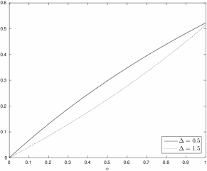
Figure 1: ‘Hadamard derivative’ $\dot{\cal V}_{0;\boldsymbol{P}}^{x_{0}}(\boldsymbol{Q}_{\Delta,\tau}-\boldsymbol{P})$ (for $\Delta=1.5)$ and negative ‘Hadamard derivative’ $-\dot{\cal V}_{0;\boldsymbol{P}}^{x_{0}}(\boldsymbol{Q}_{\Delta,\tau}-\boldsymbol{P})$ (for $\Delta=0.5)$ for $N=12$, $\nu=0.01$, $\mu_{\boldsymbol{P}}=0.05$, and $\sigma_{\boldsymbol{P}}=0.2$ in dependence of the risk aversion parameter $\alpha$.

As appears from Figure 1 the negative effect of incorporating a ‘jump’ $\Delta=0.5$ in the dynamics $S=(S_{0},\ldots,S_{N})$ of an asset price is larger than the positive effect of incorporating a ‘jump’ $\Delta=1.5$ for every choice of the agent’s degree of risk aversion. Figure 1 also shows the unsurprising effect that a high risk aversion (small value of $\alpha$) leads to a negligible sensitivity.

Next we compare the values of $\dot{\cal V}_{0;\boldsymbol{P}}^{x_{0}}(\boldsymbol{Q}_{\Delta,\tau}-\boldsymbol{P})$ for trading horizons $N\in\{4,12,52\}$ in dependence of the drift $\nu$ of the bond and the ‘jump’ $\Delta$. This choices of $N$ correspond respectively to a quarterly, monthly, and weekly time discretization. We will restrict ourselves to ‘jumps’ $\Delta\leq 0.8$. On the one hand, this ensures that the ‘jumps’ are significant; see the discussion above. On the other hand, as just discerned from Figure 1, the effect of jumps ‘down’ are more significant than jumps ‘up’.

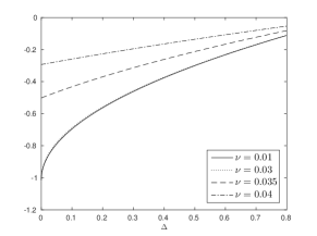
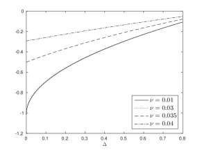
Figure 2: ‘Hadamard derivative’ $\dot{\cal V}_{0;\boldsymbol{P}}^{x_{0}}(\boldsymbol{Q}_{\Delta,\tau}-\boldsymbol{P})$ for $\alpha=0.5$, $\mu_{\boldsymbol{P}}=0.05$, and $\sigma_{\boldsymbol{P}}=0.2$ in dependence of the ‘jump’ $\Delta$ and the drift $\nu$ of the bond, showing $N=4$ in the first, $N=12$ in the second, and $N=52$ in the third column.

From Figure 2 one can see that for each trading time $N$ and any $\Delta\in[0,0.8]$ the (negative) effect of incorporating a ‘jump’ $\Delta$ in the dynamics $S=(S_{0},\ldots,S_{N})$ of an asset price is the smaller the smaller the spread between the drift $\mu_{\boldsymbol{P}}$ of the asset and the drift $\nu$ of the bond. There is only a tiny (nearly invisible) difference between the ‘Hadamard derivative’ $\dot{\cal V}_{0;\boldsymbol{P}}^{x_{0}}(\boldsymbol{Q}_{\Delta,\tau}-\boldsymbol{P})$ for the trading times $N\in\{4,12,52\}$. So the fineness of the discretization seems to play a minor part. Next we compare the values of $\dot{\cal V}_{0;\boldsymbol{P}}^{x_{0}}(\boldsymbol{Q}_{\Delta,\tau}-\boldsymbol{P})$ for the drift $\nu\in\{0.02,0.03,0.04\}$ of the bond in dependence of the risk aversion parameter $\alpha$ and the ‘jump’ $\Delta$.

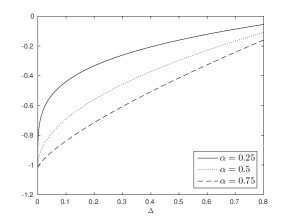
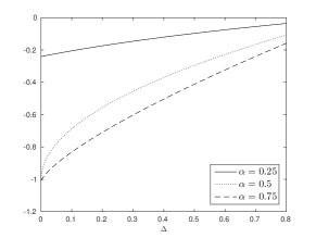
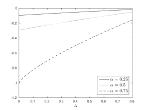
Figure 3: ‘Hadamard derivative’ $\dot{\cal V}_{0;\boldsymbol{P}}^{x_{0}}(\boldsymbol{Q}_{\Delta,\tau}-\boldsymbol{P})$ for $N=12$, $\mu_{\boldsymbol{P}}=0.05$, and $\sigma_{\boldsymbol{P}}=0.2$ in dependence of the ‘jump’ $\Delta$ and risk aversion parameter $\alpha$, showing $\nu=0.02$ in the first, $\nu=0.03$ in the second, and $\nu=0.04$ in the third column.

As appears from Figure 3, for any $\Delta\in[0,0.8]$ the (negative) effect of incorporating a ‘jump’ $\Delta$ in the dynamics $S=(S_{0},\ldots,S_{N})$ of an asset price is the smaller the higher the agent’s risk aversion, no matter what the drift $\nu\in\{0.02,0.03,0.04\}$ of the bond looks like. Take into account that the extent of this effect is influenced via (41)–(47) by the optimal fraction $\gamma^{\boldsymbol{P}}_{\mathsf{B}SM}$ to be invested into the asset which in turn depends on the risk aversion parameter $\alpha$ (see (36)).

Finally, let us briefly touch on the case where more than one jump may appear. More precisely, instead of $\boldsymbol{Q}_{\Delta,\tau}$ (with $\tau\in\{0,\ldots,N-1\}$) consider the transition function $\boldsymbol{Q}_{\Delta,\boldsymbol{\tau}(\ell)}$ (with $1\leq\ell\leq N$, $\boldsymbol{\tau}(\ell)=(\tau_{1},\ldots,\tau_{\ell})$, $\tau_{1},\ldots,\tau_{\ell}\in\{0,\ldots,N-1\}$ pairwise distinct) which is still generated by means of (40) but with the difference that at the $\ell$ different times $\tau_{1},\ldots,\tau_{\ell}$ the distribution $\mathfrak{m}_{\boldsymbol{P}}$ is replaced by $\delta_{\Delta}$. Just as in the case $\ell=1$, it turns out that it does not matter at which times $\tau_{1},\ldots,\tau_{\ell}$ exactly these $\ell$ jumps occur. Figure 4 shows the value of $\dot{\cal V}_{0;\boldsymbol{P}}^{x_{0}}(\boldsymbol{Q}_{\Delta,\boldsymbol{\tau}(\ell)}-\boldsymbol{P})$ in dependence on $\ell$ and $\Delta$. It seems that for any fixed $\Delta\in[0,0.8]$ the first-order sensitivity increases approximately linearly in $\ell$.

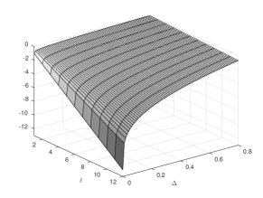
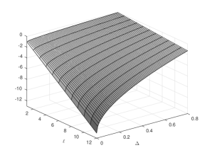
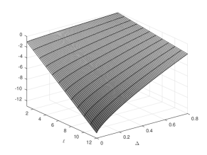
Figure 4: ‘Hadamard derivative’ $\dot{\cal V}_{0;\boldsymbol{P}}^{x_{0}}(\boldsymbol{Q}_{\Delta,\boldsymbol{\tau}(\ell)}-\boldsymbol{P})$ for $N=12$ in dependence of $\ell\in\{1,\ldots,N\}$ and $\Delta\in[0,0.8]$ showing $\alpha=0.25$ and $\nu=0.02$ (left), $\alpha=0.5$ and $\nu=0.03$ (middle), and $\alpha=0.75$ and $\nu=0.04$ (right).

Supplementary material

The supplementary material illustrates the setting of Sections 2–3 in the case of finite state space and action spaces, and contains the proofs of the results from Sections 3–4. Moreover, supplemental definitions and results to Section 2 are given and the existence of optimal strategies in general MDMs is discussed. Finally, an supplemental topological result is shown.

5 Supplement: The discrete case as an illustrating example

In Sections 2–3 we work in a rather general set-up. This implies that we cannot avoid dealing with ‘advanced’ objects. In the special case where the state space and the action spaces are finite the situation is different. In this case it is possible to present the basic definitions and the main result (Theorem 3.14) in a more comprehensible way. For the moment we assume that the reader is already familiar with the basic terminology of MDMs. Otherwise we advise the reader to first read Section 2. In Section 5.5 it will be discussed how the following elaborations fit to the general set-up of Sections 2–3.

5.1 Basic model components

Let $E=\{x_{1},\ldots,x_{\mathfrak{s}}\}$ be a finite state space, $N\in\mathbb{N}$ be a fixed finite time horizon, and $A_{n}(x_{i})=\{a_{n,i;1},\ldots,a_{n,i;\mathfrak{t}_{n,i}}\}$ be the finite set of possible actions that can be performed when the MDP is in state $x_{i}$ at time $n\in\{0,\ldots,N-1\}$. For any $n=0,\ldots,N-1$, $i=1,\ldots,\mathfrak{s}$, and $a\in A_{n}(x_{i})$, the (one-step transition) probability measure on $E$ from which the state of the MDP at time $n+1$ is drawn, given that the MDP is in state $x_{i}$ and action $a$ is selected at time $n$, can be identified with an element $p_{n,i;a}=(p_{n,i;a}(1),\ldots,p_{n,i;a}(\mathfrak{s}))$ of $\mathbb{R}_{\geq 0,1}^{\mathfrak{s}}$. Here $\mathbb{R}_{\geq 0,1}^{\mathfrak{s}}$ is the set of all vectors from $\mathbb{R}^{\mathfrak{s}}$ whose entries are nonnegative and sum up to $1$, and $p_{n,i;a}(j)$ specifies the probability that the MDP will be in state $x_{j}$ at time $n+1$, given it is in state $x_{i}$ and action $a\in A_{n}(x_{i})$ is selected at time $n$. In particular, if the initial state $x_{0}\in E$ is fixed and $i_{0}$ refers to the corresponding index (i.e. $x_{0}=x_{i_{0}}$), the vector

$$\boldsymbol{p}:=\big{(}\oplus_{k=1}^{\mathfrak{t}_{0,i_{0}}}p_{0,i_{0};a_{0,i_{0};k}}\big{)}\oplus\big{(}\oplus_{n=1}^{N-1}\oplus_{i=1}^{\mathfrak{s}}\oplus_{k=1}^{\mathfrak{t}_{n,i}}p_{n,i;a_{n,i;k}}\big{)}$$ (48)

in $\mathbb{R}^{\mathfrak{d}}$, with $\mathfrak{d}:=(\mathfrak{t}_{0,i_{0}}+\sum_{n=1}^{N-1}\sum_{i=1}^{\mathfrak{s}}\mathfrak{t}_{n,i})\mathfrak{s}$, can be identified with the transition probability function, i.e. with the ensemble of all transition probabilities. Here $\oplus$ is the ‘clueing operator’ defined by $(\alpha_{1},\ldots,\alpha_{s})\oplus(\beta_{1},\ldots,\beta_{t}):=(\alpha_{1},\ldots,\alpha_{s},\beta_{1},\ldots,\beta_{t})$. In fact $\boldsymbol{p}$ is even an element of the following subset of $\mathbb{R}^{\mathfrak{d}}$:

$$\widetilde{\cal P}:=\big{(}\mathbb{R}_{\geq 0,1}^{\mathfrak{s}}\big{)}^{\times(\mathfrak{d}/\mathfrak{s})}.$$ (49)

If ${\cal V}_{0}(\boldsymbol{p})$ denotes the optimal value of the MDM based on transition probability function $\boldsymbol{p}$, then ${\cal V}_{0}={\cal V}_{0}(\cdot)$ can be seen as a map from $\widetilde{\cal P}$ ($\subseteq\mathbb{R}^{\mathfrak{d}}$) to $\mathbb{R}$.

5.2 Definition of first-order sensitivity in the discrete case

It is tempting to consider the classical Fréchet (or total) derivative $\dot{\cal V}_{0;\boldsymbol{p}}$ of ${\cal V}_{0}$ at $\boldsymbol{p}$ in order to obtain a tool for measuring the first-order sensitivity of the optimal value w.r.t. a change from $\boldsymbol{p}$ to $(1-\varepsilon)\boldsymbol{p}+\varepsilon\boldsymbol{q}$:

$$\dot{\cal V}_{0;\boldsymbol{p}}(\boldsymbol{q}-\boldsymbol{p})=\lim_{m\to\infty}\frac{{\cal V}_{0}(\boldsymbol{p}+h_{m}(\boldsymbol{q}-\boldsymbol{p}))-{\cal V}_{0}(\boldsymbol{p})}{h_{m}}\quad\mbox{ uniformly in }\boldsymbol{q}\in\overline{B}_{1}(\boldsymbol{p})$$ (50)

for any $(h_{m})\in\mathbb{R}_{0}^{\mathbb{N}}$ with $h_{m}\to 0$, where $\overline{B}_{1}(\boldsymbol{p})$ is the closed ball in $\mathbb{R}^{\mathfrak{d}}$ around $\boldsymbol{p}$ with radius $1$ and $\mathbb{R}_{0}:=\mathbb{R}\setminus\{0\}$. This approach is indeed expedient to some extent. However, one has to note that $\boldsymbol{p}+h_{m}(\boldsymbol{q}-\boldsymbol{p})$ may lie outside ${\cal V}_{0}$’s domain $\widetilde{\cal P}$. To avoid this problem, we replace condition (50) by the following variant of (50):

$$\dot{\cal V}_{0;\boldsymbol{p}}(\boldsymbol{q}-\boldsymbol{p})=\lim_{m\to\infty}\frac{{\cal V}_{0}(\boldsymbol{p}+\varepsilon_{m}(\boldsymbol{q}-\boldsymbol{p}))-{\cal V}_{0}(\boldsymbol{p})}{\varepsilon_{m}}\quad\mbox{ uniformly in }\boldsymbol{q}\in\widetilde{\cal P}$$ (51)

for any $(\varepsilon_{m})\in(0,1]^{\mathbb{N}}$ with $\varepsilon_{m}\to 0$. Take into account that $\boldsymbol{p}+\varepsilon(\boldsymbol{q}-\boldsymbol{p})$ lies in $\widetilde{\cal P}$ for any $\boldsymbol{p},\boldsymbol{q}\in\widetilde{\cal P}$ and $\varepsilon\in(0,1]$. Also note that, if $\mathbb{R}^{\mathfrak{d}}$ is equipped with the max-norm, $\widetilde{\cal P}$ is contained in $\overline{B}_{1}(\boldsymbol{p})$ for any $\boldsymbol{p}\in\widetilde{\cal P}$.

For classical Fréchet (or total) differentiability the derivative $\dot{\cal V}_{0;\boldsymbol{p}}$ is required to be linear and continuous. On the one hand, for ‘Fréchet differentiability’ (see Definition 5.1) we will also require a sort of continuity, namely that the mapping $\boldsymbol{q}\mapsto\dot{\cal V}_{0;\boldsymbol{p}}(\boldsymbol{q}-\boldsymbol{p})$ from $\widetilde{\cal P}$ to $\mathbb{R}$ is continuous, where $\widetilde{\cal P}$ is equipped with the relative topology of $\mathbb{R}^{\mathfrak{d}}$. On the other hand, the domain of $\dot{\cal V}_{0;\boldsymbol{p}}$ is given by $\widetilde{\cal P}^{\boldsymbol{p};\pm}:=\{\boldsymbol{q}-\boldsymbol{p}:\boldsymbol{q}\in\widetilde{\cal P}\}$ and thus not a linear space. Therefore linearity of $\dot{\cal V}_{0;\boldsymbol{p}}$ is an indefinite property.

In view of (1), the quantity $\dot{\cal V}_{0;\boldsymbol{p}}(\boldsymbol{q}-\boldsymbol{p})$ can be seen as a measure for the first-order sensitivity of the optimal value ${\cal V}_{0}(\boldsymbol{p})$ under transition probability function $\boldsymbol{p}$ w.r.t. a change from $\boldsymbol{p}$ to $(1-\varepsilon)\boldsymbol{p}+\varepsilon\boldsymbol{q}$, with $\varepsilon>0$ small. For this interpretation it is actually not necessary to require that $\dot{\cal V}_{0;\boldsymbol{p}}(\,\cdot\,-\boldsymbol{p})$ is continuous or that the convergence in (51) holds uniformly in $\boldsymbol{q}\in\widetilde{\cal P}$. One can indeed be content with the directional derivative, i.e. with the convergence in (51) for fixed $\boldsymbol{q}$. Nevertheless continuity and uniformity are natural wishes in this context, because they ensure stability of the first-order sensitivity w.r.t. small modifications of $\boldsymbol{q}$ as well as comparability of the first-order sensitivity of (infinitely) many different $\boldsymbol{q}$. We refer to the discussion subsequent to (1).

Definition 5.1

A map ${\cal V}:\widetilde{\cal P}\rightarrow\mathbb{R}$ is said to be ‘Fréchet differentiable’ at $\boldsymbol{p}\in\widetilde{\cal P}$ if there exists a map $\dot{\cal V}_{\boldsymbol{p}}:\widetilde{\cal P}^{\boldsymbol{p};\pm}\to\mathbb{R}$ for which (51) (with ${\cal V}_{0},\dot{\cal V}_{0;\boldsymbol{p}}$ replaced by ${\cal V},\dot{\cal V}_{\boldsymbol{p}}$ respectively) holds and for which the mapping $\boldsymbol{q}\mapsto\dot{\cal V}_{\boldsymbol{p}}(\boldsymbol{q}-\boldsymbol{p})$ from $\widetilde{\cal P}$ to $\mathbb{R}$ is continuous. In this case $\dot{\cal V}_{\boldsymbol{p}}$ is called ‘Fréchet derivative’ of ${\cal V}$ at $\boldsymbol{p}$.

5.3 Computation of first-order sensitivity in the discrete case

To specify the ‘Fréchet derivative’ of ${\cal V}_{0}$ at $\boldsymbol{p}$ we need some further notation. For any strategy $\pi=(f_{n})_{n=0}^{N-1}$, we use ${\cal V}_{0}^{\pi}(\boldsymbol{p})$ to denote the expected total reward (from time $0$ to $N$) when $\boldsymbol{p}$ is the underlying transition probability function and the decisions are performed according to $\pi$. In the finite setting there exists under $\boldsymbol{p}$ at least one optimal strategy $\pi^{\boldsymbol{p}}$, i.e. a strategy $\pi^{\boldsymbol{p}}$ with ${\cal V}_{0}^{\pi^{\boldsymbol{p}}}(\boldsymbol{p})=\max_{\pi}{\cal V}_{0}^{\pi}(\boldsymbol{p})$. We will write $\Pi(\boldsymbol{p})$ for the (finite) set of all optimal strategies w.r.t. $\boldsymbol{p}$. Then the results of Subsection 3.5 show that the ‘Fréchet derivative’ of ${\cal V}_{0}$ at $\boldsymbol{p}$ is given by

$$\dot{\cal V}_{0;\boldsymbol{p}}(\boldsymbol{q}-\boldsymbol{p})=\max_{\pi\in\Pi(\boldsymbol{p})}\dot{\cal V}_{0;\boldsymbol{p}}^{\pi}(\boldsymbol{q}-\boldsymbol{p})\quad\mbox{ for all }\boldsymbol{q}\in\widetilde{\cal P},$$ (52)

where $\dot{\cal V}_{0;\boldsymbol{p}}^{\pi}$ refers to the ‘Fréchet derivative’ of ${\cal V}_{0}^{\pi}$ at $\boldsymbol{p}$. The latter can be obtained from a suitable iteration scheme. According to Remark 3.19 we indeed have

$$\dot{\cal V}_{0;\boldsymbol{p}}^{\pi}(\boldsymbol{q}-\boldsymbol{p})=\dot{V}_{0}^{\boldsymbol{p},\boldsymbol{q};\pi}(x_{i_{0}})$$

(recall that $x_{i_{0}}\in E$ is the initial state and that $\pi=(f_{n})_{n=0}^{N-1}$ refers to a strategy) for

$$\dot{V}_{N}^{\boldsymbol{p},\boldsymbol{q};\pi}(x_{i}) \,:=\,0$$ (53)

$$\dot{V}_{n}^{\boldsymbol{p},\boldsymbol{q};\pi}(x_{i}) \,:=\,\sum_{j=1}^{\mathfrak{s}}\dot{V}_{n+1}^{\boldsymbol{p},\boldsymbol{q};\pi}(x_{j})\,p_{n,i;f_{n}(x_{i})}(j)$$

$$\qquad+\sum_{j=1}^{\mathfrak{s}}V^{\boldsymbol{p};\pi}_{n+1}(x_{j})\,\big{(}q_{n,i;f_{n}(x_{i})}(j)-p_{n,i;f_{n}(x_{i})}(j)\big{)},\quad n=0,\ldots,N-1,$$

$i=1,\ldots,\mathfrak{s}$, where the $V^{\boldsymbol{p};\pi}_{n}(\cdot)$ are given by the usual backward iteration scheme (see, e.g., Lemma 3.5 in [13] or p. 80 in [30]) for the computation of ${\cal V}^{\pi}_{0}(\boldsymbol{p})$:

$$V_{N}^{\boldsymbol{p};\pi}(x_{i}) \,:=\,r_{N}(x_{i})$$ (54)

$$V_{n}^{\boldsymbol{p};\pi}(x_{i}) \,:=\,r_{n}(x_{i},f_{n}(x_{i}))+\sum_{j=1}^{\mathfrak{s}}V_{n+1}^{\boldsymbol{p};\pi}(x_{j})\,p_{n,i;f_{n}(x_{i})}(j),\quad n=0,\ldots,N-1,$$

$i=1,\ldots,\mathfrak{s}$. Here $r_{n}(x_{i},a)$ specifies the (one-stage) reward when making decision $a$ at time $n$ in state $x_{i}$, and $r_{N}(x_{i})$ specifies the reward of being in state $x_{i}$ at terminal time $N$. Also note that $f_{n}(x_{i})$ determines the action which is taken at time $n$ in state $x_{i}$ under strategy $\pi=(f_{n})_{n=0}^{N-1}$.

5.4 An example: stochastic inventory control

In this subsection we will consider an inventory control problem, which is a classical example in discrete dynamic optimization; see, e.g., [5, 12, 30] and references cited therein. At first, we introduce in Subsection 5.4.1 a (simple) inventory control model and formulate the corresponding inventory control problem. Thereafter, in Subsection 5.4.2, we will explain how the inventory control model can be embedded into the setting of Subsection 5.1. Finally, in Subsection 5.4.3 we will present some numerical examples for the ‘Fréchet derivative’ established in Subsection 5.3.

5.4.1 Basic inventory control model, and the target

Consider an $N$-period inventory control system where a supplier of a single product seeks optimal inventory management to meet random commodity demand in such a way that a measure of profit over a time horizon of $N$ periods is maximized. For the formulation of the model, let $I_{1},\ldots,I_{N}$ be $\mathbb{N}_{0}$-valued independent random variables on some probability space $(\Omega,{\cal F},\mathbb{P})$, where $I_{n+1}$ can be seen as the random demand of the single product in the period between time $n$ and time $n+1$. We denote by $\mathfrak{p}_{n+1}=(\mathfrak{p}_{n+1;k})_{k\in\mathbb{N}_{0}}$ the counting density of $I_{n+1}$ (i.e. $\mathfrak{p}_{n+1;k}:=\mathbb{P}[I_{n+1}=k]$) and assume that $\mathfrak{p}_{n+1}$ is known for any $n=0,\ldots,N-1$. Note that $\mathfrak{p}_{n+1}\in\mathbb{R}_{\geq 0,1}^{\mathbb{N}_{0}}$, where $\mathbb{R}_{\geq 0,1}^{\mathbb{N}_{0}}$ denotes the space of all real-valued sequences whose entries are nonnegative and sum up to $1$. Let ${\cal F}_{0}$ be the trivial $\sigma$-algebra, and set ${\cal F}_{n}:=\sigma(I_{1},\ldots,I_{n})$ for any $n=1,\ldots,N$.

We suppose that within each period of time the available inventory level of the single product is restricted to $K$ units (for some fixed $K\in\mathbb{N}$) and that there is no backlogging of unsatisfied demand at the end of each period. The latter means that if at the end of a period the demand exceeds the current inventory, then the whole inventory is sold and the surplus demand gets lost.

Given an initial inventory level $y_{0}\in\{0,\ldots,K\}$, the supplier intends to find optimal order quantities according to an order strategy to maximize some measure of profit. By order strategy we mean an (${\cal F}_{n}$)-adapted $\{0,\ldots,K\}$-valued stochastic process $\varphi=(\varphi_{n})_{n=0}^{N-1}$, where $\varphi_{n}$ specifies the amount of ordered units of the single product at the beginning of period $n$. Here we suppose that the delivery of any order occurs instantaneously. Since excess demand is lost by assumption, the corresponding inventory (level) process $Y^{\varphi}=(Y^{\varphi}_{0},\ldots,Y^{\varphi}_{N})$ associated with $\varphi=(\varphi_{n})_{n=0}^{N-1}$ is given by

$$Y^{\varphi}_{0}:=y_{0}\quad\mbox{ and }\quad Y^{\varphi}_{n+1}:=Y^{\varphi}_{n}+\varphi_{n}-\min\{I_{n+1},Y^{\varphi}_{n}+\varphi_{n}\},\qquad n=0,\ldots,N-1.$$ (55)

Note that $\min\{I_{n+1},Y^{\varphi}_{n}+\varphi_{n}\}$ corresponds to the amount of units of the single product sold in the period between time $n$ and time $n+1$. Hence we refer to the process $Z^{\varphi}:=(Z^{\varphi}_{0},\ldots,Z^{\varphi}_{N})$ defined by

$$Z^{\varphi}_{0}:=0\quad\mbox{ and }\quad Z^{\varphi}_{n+1}:=\min\{I_{n+1},Y^{\varphi}_{n}+\varphi_{n}\},\qquad n=0,\ldots,N-1$$ (56)

as sales process associated with $\varphi=(\varphi_{n})_{n=0}^{N-1}$.

In view of (55) and since the inventory capacity is restricted to $K$ units, we may and do identify any order strategy with an (${\cal F}_{n}$)-adapted $\{0,\ldots,K\}$-valued stochastic process $\varphi=(\varphi_{n})_{n=0}^{N-1}$ satisfying $\varphi_{0}\in\{0,\ldots,K-y_{0}\}$ and $\varphi_{n}\in\{0,\ldots,K-Y^{\varphi}_{n}\}$ for all $n=1,\ldots,N-1$. We restrict ourselves to Markovian order strategies $\varphi=(\varphi_{n})_{n=0}^{N-1}$ which means that $\varphi_{n}$ only depends on $n$ and $(Y^{\varphi}_{n},Z^{\varphi}_{n})$. To put it another way, we suppose that for any $n=0,\ldots,N-1$ there is some map $f_{n}:\{0,\ldots,K\}^{2}\to\{0,\ldots,K\}$ such that $\varphi_{n}=f_{n}(Y^{\varphi}_{n},Z^{\varphi}_{n})$. Hence, for given strategy $\varphi=(\varphi_{n})_{n=0}^{N-1}$ (resp. $\pi=(f_{n})_{n=0}^{N-1}$) the process $X^{\varphi}:=(Y^{\varphi},Z^{\varphi})$ is a $\{0,\ldots,K\}^{2}$-valued $({\cal F}_{n})$-Markov process whose one-step transition probability for the transition from state $x=(y,z)\in\{0,\ldots,K\}^{2}$ at time $n\in\{0,\ldots,N-1\}$ to state $x^{\prime}=(y^{\prime},z^{\prime})\in\{0,\ldots,K\}^{2}$ at time $n+1$ is given by $\eta^{\mathfrak{p}_{n+1}}_{(y,f_{n}(y,z))}(z^{\prime})\mathbbm{1}_{\{y^{\prime}=y+f_{n}(y,z)-z^{\prime}\}}$ with

$$\eta^{\mathfrak{p}_{n+1}}_{(y,a)}(z^{\prime}):=\left\{\begin{array}[]{lll}0&,&z^{\prime}>y+a\\ \mathfrak{p}_{n+1;z^{\prime}}&,&z^{\prime}<y+a\\ \sum_{\ell=z^{\prime}}^{\infty}\mathfrak{p}_{n+1;\ell}&,&z^{\prime}=y+a\end{array}\right..$$ (57)

The supplier’s aim is to find an order strategy $\varphi=(\varphi_{n})_{n=0}^{N-1}$ (resp. $\pi=(f_{n})_{n=0}^{N-1}$) for which the expected total profit is maximized. Here the profit can be seen as the difference between the sales revenue and the costs for ordering and holding the single product. For the sake of simplicity, we suppose that the sales revenue as well as the ordering and holding costs are known and linear in each period. Hence, we are interested in those order strategies $\varphi=(\varphi_{n})_{n=0}^{N-1}$ (resp. $\pi=(f_{n})_{n=0}^{N-1}$) for which the expectation of

$$\sum_{k=0}^{N-1}\big{\{}u^{\mathsf{r}ev}(Z_{k}^{\varphi})-u^{\mathsf{o}rd}(f_{k}(Y_{k}^{\varphi},Z_{k}^{\varphi}))-u^{\mathsf{h}ol}(Y_{k}^{\varphi},f_{k}(Y_{k}^{\varphi},Z_{k}^{\varphi}))\big{\}}+\big{\{}u^{\mathsf{r}ev}(Z_{N}^{\varphi})-u^{\mathsf{h}ol}(Y_{N}^{\varphi},0)\big{\}}$$

is maximized, where $u^{\mathsf{r}ev},u^{\mathsf{o}rd}:\{0,\ldots,K\}\to\mathbb{N}_{0}$ and $u^{\mathsf{h}ol}:\{0,\ldots,K\}^{2}\to\mathbb{N}_{0}$ are for some fixed $s_{\mathsf{r}ev},c_{\mathsf{o}rd},c_{\mathsf{f}ix},c_{\mathsf{h}ol}\in\mathbb{N}$ defined by

$$u^{\mathsf{r}ev}(z):=s_{\mathsf{r}ev}\cdot z,\quad u^{\mathsf{o}rd}(a):=(c_{\mathsf{f}ix}+c_{\mathsf{o}rd}\cdot a)\mathbbm{1}_{\{a>0\}},\quad u^{\mathsf{h}ol}(y,a):=c_{\mathsf{h}ol}\cdot(y+a).$$

Note here that $s_{\mathsf{r}ev},c_{\mathsf{o}rd},c_{\mathsf{f}ix}$, and $c_{\mathsf{h}ol}$ denote the sales revenue, the ordering costs, the fixed ordering costs, and the holding costs per unit of the single product, respectively.

5.4.2 Embedding into MDM, and optimal order strategies

The setting introduced in Subsection 5.4.1 can be embedded into the setting of Subsections 5.1 and 5.3 as follows. Let $E:=\{x_{1},\ldots,x_{\mathfrak{s}}\}$ for the enumeration $x_{1},\ldots,x_{\mathfrak{s}}$ (with $\mathfrak{s}=(K+1)^{2}$) of $\{0,\ldots,K\}^{2}$ given by $x_{i}=(y_{i},z_{i})$ with $y_{i}:=\lceil i/(K+1)\rceil-1$ and $z_{i}:=i-(K+1)\lceil i/(K+1)\rceil+K$ (here $\lceil\cdot\rceil$ is the ceiling function), $i=1,\ldots,\mathfrak{s}$.

Let $A_{n}(x_{i}):=\{a_{n,i;1},\ldots,a_{n,i;\mathfrak{t}_{n,i}}\}$ with $a_{n,i;k}:=k-1$ and $\mathfrak{t}_{n,i}=\mathfrak{t}_{i}:=K-y_{i}+1$ for any $i=1,\ldots,\mathfrak{s}$ and $n=0,\ldots,N-1$. For any $i=1,\ldots,\mathfrak{s}$, $k=1,\ldots,\mathfrak{t}_{i}$, and $n=0,\ldots,N-1$, let the component $p_{n,i;a_{n,i;k}}=(p_{n,i;a_{n,i;k}}(1),\break\ldots,p_{n,i;a_{n,i;k}}(\mathfrak{s}))$ of the vector $\boldsymbol{p}$ from (48) be given by

$$p_{n,i;a_{n,i;k}}(j):=\eta^{\mathfrak{p}_{n+1}}_{(y_{i},a_{n,i;k})}(z_{j})\mathbbm{1}_{\{y_{j}=y_{i}+a_{n,i;k}-z_{j}\}},\qquad j=1,\ldots,\mathfrak{s}$$ (58)

for some predetermined $\mathfrak{p}_{n+1}\in\mathbb{R}_{\geq 0,1}^{\mathbb{N}_{0}}$ and for $\eta^{\mathfrak{p}_{n+1}}_{(y,a)}(\cdot)$ introduced in (57). In fact any element $\boldsymbol{p}$ of $\widetilde{\cal P}$ is generated via (57)–(58) by some $N$-tuple $\mathfrak{p}=(\mathfrak{p}_{1},\ldots,\mathfrak{p}_{N})$ of counting densities $\mathfrak{p}_{1},\ldots,\mathfrak{p}_{N}$ on $\mathbb{N}_{0}$; here $\mathfrak{p}_{1},\ldots,\mathfrak{p}_{N}$ should be seen as the counting densities of $I_{1},\ldots,I_{N}$. The value in (58) should be seen as the probability of a transition from state $(y_{i},z_{i})$ to state $(y_{j},z_{j})$ in time between $n$ and $n+1$ (this transition probability is even independent of $z_{i}$).

For any $i=1,\ldots,\mathfrak{s}$ and $k=1,\ldots,\mathfrak{t}_{i}$, set

$$r_{0}(x_{i},a_{0,i;k}) := -u^{\mathsf{o}rd}(a_{0,i;k})-u^{\mathsf{h}ol}(y_{i},a_{0,i;k}),\hskip 21.33955pt$$ (59)

$$r_{n}(x_{i},a_{n,i;k}) := u^{\mathsf{r}ev}(z_{i})-u^{\mathsf{o}rd}(a_{n,i;k})-u^{\mathsf{h}ol}(y_{i},a_{n,i;k}),\ n=1,\ldots,N-1,\hskip 21.33955pt$$ (60)

$$r_{N}(x_{i}) := u^{\mathsf{r}ev}(z_{i})-u^{\mathsf{h}ol}(y_{i},0).\hskip 21.33955pt$$ (61)

By an (admissible) order strategy we understand an $N$-tuple $\pi=(f_{n})_{n=0}^{N-1}$ of maps $f_{n}:\{x_{1},\ldots,x_{\mathfrak{s}}\}\to\{0,\ldots,K\}$ satisfying

$$f_{n}(x_{i})=f_{n}(y_{i},z_{i})\in\{0,\ldots,K-y_{i}\}\quad\mbox{ for all }i=1,\ldots,\mathfrak{s}.$$

Then for every fixed $\boldsymbol{p}\in\widetilde{\cal P}$ the inventory control problem introduced in Subsection 5.4.1 reads as

$${\cal V}_{0}^{\pi}(\boldsymbol{p})\longrightarrow\max\ (\mbox{in $\pi$)\,!}$$ (62)

where ${\cal V}_{0}^{\pi}(\boldsymbol{p}):=V_{0}^{\boldsymbol{p};\pi}(x_{i_{0}})$ is given by (54) with (59)–(61) ($x_{i_{0}}\in E$ is the initial state). A strategy $\pi^{\boldsymbol{p}}$ is called an optimal order strategy w.r.t. $\boldsymbol{p}$ if it solves the maximization problem (62).

5.4.3 Numerical examples for the ‘Fréchet derivative’

Let us take up the numerical example at p. 41 in [30] where $N:=3$, $K:=4$, $s_{\mathsf{r}ev}:=8$, $c_{\mathsf{o}rd}:=2$, $c_{\mathsf{f}ix}:=4$, and $c_{\mathsf{h}ol}:=1$. We fix $\mathfrak{p}:=(\mathfrak{p}_{\bullet},\mathfrak{p}_{\bullet},\mathfrak{p}_{\bullet})$ with $\mathfrak{p}_{\bullet}:=(0,\tfrac{1}{4},\tfrac{1}{2},\tfrac{1}{4},0,0\ldots)$, and denote by $\boldsymbol{p}$ the unique element of $\widetilde{\cal P}$ generated by $\mathfrak{p}$ through (57)–(58). This choice of $\mathfrak{p}$ means that in each period the demand is $1$, $2$, or $3$ with probability $\tfrac{1}{4}$, $\tfrac{1}{2}$, and $\tfrac{1}{4}$, respectively. Table 2 provides the (unique) optimal order strategy $\pi^{\boldsymbol{p}}=(f_{0}^{\boldsymbol{p}},f_{1}^{\boldsymbol{p}},f_{2}^{\boldsymbol{p}})$, and the second column of Table 3 displays the maximal expected total reward ${\cal V}^{\pi^{\boldsymbol{p}}}_{0}(\boldsymbol{p})$ of the inventory control problem (62) for all possible initial inventory levels $y_{0}:=y_{i_{0}}\in\{0,\ldots,4\}$. Moreover, the last two columns in Table 3 display the ‘Fréchet derivative’ $\dot{\cal V}^{\pi^{\boldsymbol{p}}}_{0;\boldsymbol{p}}(\cdot)$ of ${\cal V}^{\pi^{\boldsymbol{p}}}_{0}$ at $\boldsymbol{p}$ evaluated at direction $\boldsymbol{q}_{(0)}-\boldsymbol{p}$ and at direction $\boldsymbol{q}_{(4)}-\boldsymbol{p}$ (calculated with the iteration scheme (53)), again for all possible initial inventory levels $y_{0}$. Here $\boldsymbol{q}_{(0)}$ and $\boldsymbol{q}_{(4)}$ are generated through (57)–(58) by $\mathfrak{q}_{(0)}:=(\mathfrak{q}_{(0)\bullet},\mathfrak{q}_{(0)\bullet},\mathfrak{q}_{(0)\bullet})$ and $\mathfrak{q}_{(4)}:=(\mathfrak{q}_{(4)\bullet},\mathfrak{q}_{(4)\bullet},\mathfrak{q}_{(4)\bullet})$ respectively, where $\mathfrak{q}_{(0)\bullet}:=(1,0,0,\ldots)$ and $\mathfrak{q}_{(4)\bullet}:=(0,0,0,0,1,0,0,\ldots)$. As the optimal strategy $\pi^{\boldsymbol{p}}$ is unique in our example, we even have $\dot{\cal V}_{0;\boldsymbol{p}}(\cdot)=\dot{\cal V}^{\pi^{\boldsymbol{p}}}_{0;\boldsymbol{p}}(\cdot)$.

Note that for $i\in\{0,4\}$ the value $\dot{\cal V}_{0;\boldsymbol{p}}(\boldsymbol{q}_{(i)}-\boldsymbol{p})$ (in our case it equals $\dot{\cal V}^{\pi^{\boldsymbol{p}}}_{0;\boldsymbol{p}}(\boldsymbol{q}_{(i)}-\boldsymbol{p})$) quantifies the first-order sensitivity of ${\cal V}_{0}(\boldsymbol{p})$ (respectively of ${\cal V}^{\pi^{\boldsymbol{p}}}_{0}(\boldsymbol{p})$) w.r.t. a change of the underlying probability transition function from $\boldsymbol{p}$ to $\boldsymbol{p}_{(i)}:=(1-\varepsilon)\boldsymbol{p}+\varepsilon\boldsymbol{q}_{(i)}$ with $\varepsilon\in(0,1)$ small. It can be easily seen that $\boldsymbol{p}_{(i)}$ is generated through (57)–(58) where $\mathfrak{p}:=(\mathfrak{p}_{\bullet},\mathfrak{p}_{\bullet},\mathfrak{p}_{\bullet})$ is replaced by $\mathfrak{p}_{(i)}:=(\mathfrak{p}_{(i)\bullet},\mathfrak{p}_{(i)\bullet},\mathfrak{p}_{(i)\bullet})$ with $\mathfrak{p}_{(i)\bullet}:=(1-\varepsilon)\mathfrak{p}_{\bullet}+\varepsilon\mathfrak{q}_{(i)\bullet}$ (take into account that the case differentiation in (57) does not depend on the counting density $\mathfrak{p}_{n+1}$). That is, the change from $\boldsymbol{p}$ to $\boldsymbol{p}_{(i)}$ means that the formerly impossible demand $i$ now gets assigned small but strictly positive probability $\varepsilon$ in each period.

Table 2: Optimal order strategy $\pi^{\boldsymbol{p}}=(f_{0}^{\boldsymbol{p}},f_{1}^{\boldsymbol{p}},f_{2}^{\boldsymbol{p}})$ for $\boldsymbol{p}$ as above.

$(y,z)$	$(0,0)$	$(0,1)$	$(0,2)$	$(0,3)$	$(0,4)$	$(1,0)$	$(1,1)$	$(1,2)$	$(1,3)$	$(1,4)$	$(2,0)$	$\cdots$	$(4,4)$
$f_{0}^{\boldsymbol{p}}$	4	4	4	4	4	3	3	3	3	3	0	$\cdots$	0
$f_{1}^{\boldsymbol{p}}$	4	4	4	4	4	3	3	3	3	3	0	$\cdots$	0
$f_{2}^{\boldsymbol{p}}$	2	2	2	2	2	0	0	0	0	0	0	$\cdots$	0

Table 3: Optimal value ${\cal V}^{\pi^{\boldsymbol{p}}}_{0}(\boldsymbol{p})$ and the ‘Fréchet derivative’ $\dot{\cal V}^{\pi^{\boldsymbol{p}}}_{0;\boldsymbol{p}}(\boldsymbol{q}_{(i)}-\boldsymbol{p})$ (in our example it equals $\dot{\cal V}_{0;\boldsymbol{p}}(\boldsymbol{q}_{(i)}-\boldsymbol{p})$) with $\boldsymbol{q}_{(i)}$ as above, $i\in\{0,4\}$, in dependence of the initial inventory level $y_{0}$.

$y_{0}$	${\cal V}^{\pi^{\boldsymbol{p}}}_{0}(\boldsymbol{p})$	$\dot{\cal V}^{\pi^{\boldsymbol{p}}}_{0;\boldsymbol{p}}(\boldsymbol{q}_{(0)}-\boldsymbol{p})$	$\dot{\cal V}^{\pi^{\boldsymbol{p}}}_{0;\boldsymbol{p}}(\boldsymbol{q}_{(4)}-\boldsymbol{p})$
0	16.5313	$-$34.0938	16.0313
1	18.5313	$-$34.0938	16.0313
2	23.1250	$-$39.8125	14.0000
3	26.1094	$-$37.3906	15.6094
4	28.5313	$-$34.0938	16.0313

As appears from Table 3, the negative effect of incorporating demand $0$ into the counting density $\mathfrak{p}_{\bullet}$ with small probability $\varepsilon$ is roughly twice as large as the positive effect of incorporating demand $4$ into $\mathfrak{p}_{\bullet}$ with the same small probability $\varepsilon$, no matter what the initial inventory level looks like. So, when worrying about robustness of the optimal value w.r.t. changes in the demand’s counting density $\mathfrak{p}_{\bullet}$, it seems to be somewhat more important to analyse in detail the adequacy of the assumption that an absent demand is impossible than the adequacy of the assumption that a demand of $4$ is impossible.

5.5 Embedding the discrete case into the set-up of Sections 2–3

In this subsection we will explain how the elaborations in Subsections 5.1–5.3 match our general theory introduced in Sections 2–3. Assume that the state space $E$ as well as the set of all admissible actions $A_{n}(x)$ for each point of time $n=0,\ldots,N-1$ and state $x\in E$ are finite. Let $\mathfrak{s}:=\#E\in\mathbb{N}$ and ${\cal E}:=\mathfrak{P}(E)$, and note that the sets $A_{n}$ as well as $D_{n}$ are finite for any $n=0,\ldots,N-1$.

Let us measure the distance between two probability measures $\mu$ and $\nu$ from ${\cal M}_{1}(E)$ by the total variation metric $d_{\mathrm{\scriptsize{TV}}}$, i.e. by

$$d_{\mathrm{\scriptsize{TV}}}(\mu,\nu)\,=\,\max_{B\in\mathfrak{P}(E)}\big{|}\mu[B]-\nu[B]\big{|}\,=\,\frac{1}{2}\sum_{y\in E}\big{|}\mu[\{y\}]-\nu[\{y\}]\big{|}.$$

This fits the setting of Subsection 3.2 with $\mathbb{M}:=\mathbb{M}_{\mathrm{\scriptsize{TV}}}$ and $\psi:\equiv 1$; see Example 3.3. Since $E$ was assumed to be finite with $\mathfrak{s}:=\#E\in\mathbb{N}$, we may and do identify any probability measure $\mu\in{\cal M}_{1}(E)$ with some element $p_{\mu}=(p_{\mu}(1),\ldots,p_{\mu}(\mathfrak{s}))$ of $\mathbb{R}_{\geq 0,1}^{\mathfrak{s}}$ (with $\mathbb{R}_{\geq 0,1}^{\mathfrak{s}}$ as in Subsection 5.1). Hence the total variation distance $d_{\mathrm{\scriptsize{TV}}}$ between $\mu,\nu\in{\cal M}_{1}(E)$ can be identified (up to the factor $1/2$) with the $\ell_{1}$-distance between $p_{\mu}$ and $p_{\nu}$:

$$d_{\mathrm{\scriptsize{TV}}}(\mu,\nu)\,=\,\frac{1}{2}\sum_{i=1}^{\mathfrak{s}}\big{|}p_{\mu}(i)-p_{\nu}(i)\big{|}\,=\,\frac{1}{2}\,\|p_{\mu}-p_{\nu}\|_{\ell_{1}}.$$

That is, the map $\Lambda:{\cal M}_{1}(E)\rightarrow\mathbb{R}_{\geq 0,1/2}^{\mathfrak{s}}$, $\mu\mapsto p_{\mu}/2$, provides a surjective isometry (here $\mathbb{R}_{\geq 0,1/2}^{\mathfrak{s}}$ is the set of all vectors from $\mathbb{R}^{\mathfrak{s}}$ whose entries are nonnegative and sum up to $1/2$), and therefore the metric spaces $({\cal M}_{1}(E),d_{\mathrm{\scriptsize{TV}}})$ and $(\mathbb{R}_{\geq 0,1/2}^{\mathfrak{s}},\|\cdot\|_{\ell_{1}})$ are isometrically isomorphic. This implies in particular that the set ${\cal M}_{1}(E)$ is compact w.r.t. $d_{\mathrm{\scriptsize{TV}}}$, because $\mathbb{R}_{\geq 0,1/2}^{\mathfrak{s}}$ is clearly compact w.r.t. $\|\cdot\|_{\ell_{1}}$.

For the distance between two transition functions we will employ the metric $d_{\infty,\mathbb{M}_{\mathrm{\scriptsize{TV}}}}^{1}$, which is defined as in (11) with $\psi:\equiv 1$. As the sets $D_{0},\ldots,D_{N-1}$ are finite, we can identify the set ${\cal P}$ as a finite product of ${\cal M}_{1}(E)$:

$${\cal P}\,=\,\times_{n=0}^{N-1}\times_{(x,a)\in D_{n}}{\cal M}_{1}(E).$$

The metric $d_{\infty,\mathbb{M}_{\mathrm{\scriptsize{TV}}}}^{1}$ obviously metricizes the product topology on $\overline{\cal P}_{\mathbbm{1}}={\cal P}$ and, as seen above, the set ${\cal M}_{1}(E)$ is compact w.r.t. $d_{\mathrm{\scriptsize{TV}}}$. It follows from Tychonoff’s theorem (see, e.g., [8, Theorem 2.2.8]) that ${\cal P}$ is compact w.r.t. $d_{\infty,\mathbb{M}_{\mathrm{\scriptsize{TV}}}}^{1}$ and therefore in particular relatively compact w.r.t. $d_{\infty,\mathbb{M}_{\mathrm{\scriptsize{TV}}}}^{1}$. Hence, Definition 3.11(b) of ‘Hadamard differentiability’ (i.e. Definition 3.9 with ${\cal S}:={\cal S}_{\mathrm{r}c}$) simplifies insofar as one can simply require that the convergence in (12) holds uniformly in all $\boldsymbol{Q}\in{\cal P}$ for every sequence $(\varepsilon_{m})\in(0,1]^{\mathbb{N}}$.

Under the imposed assumptions we may via (48) identify any transition function $\boldsymbol{P}=(P_{n})_{n=0}^{N-1}$ from ${\cal P}=\times_{n=0}^{N-1}\times_{(x,a)\in D_{n}}{\cal M}_{1}(E)$ with an element $\boldsymbol{p}$ of the set $\widetilde{\cal P}$ defined in (49) with $\mathfrak{d}:=(\mathfrak{t}_{0,i_{0}}+\sum_{n=1}^{N-1}\sum_{i=1}^{\mathfrak{s}}\mathfrak{t}_{n;i})\mathfrak{s}$, where $\mathfrak{t}_{n;i}:=\#A_{n}(x_{i})$ and $x_{1},\ldots,x_{\mathfrak{s}}$ is a (finite) enumeration of $E$. Then, imposing (without loss of generality) the metric

$$d_{\infty,\ell_{1}}(\boldsymbol{p},\boldsymbol{q}) :=\frac{1}{2}\max\Big{\{}\max_{k=1,\ldots,\mathfrak{t}_{0,i_{0}}}\|p_{0,i_{0};a_{0,i_{0};k}}-q_{0,i_{0};a_{0,i_{0};k}}\|_{\ell_{1}},$$

$$\qquad\qquad\qquad\max_{n=1,\ldots,N-1}\max_{i=1,\ldots,\mathfrak{s}}\max_{k=1,\ldots\mathfrak{t}_{n;i}}\|p_{n,i;a_{n,i;k}}-q_{n,i;a_{n,i;k}}\|_{\ell_{1}}\Big{\}}$$

on $\widetilde{\cal P}$, it is apparent that Definition 5.1 is a special case of Definition 3.9 with ${\cal S}:={\cal S}_{\mathrm{r}c}$.

Note that in the finite setting there exists for any fixed $\boldsymbol{P}\in{\cal P}$ an optimal strategy $\pi^{\boldsymbol{P}}\in\Pi$ w.r.t. $\boldsymbol{P}$, which means that the set $\Pi(\boldsymbol{P})$ is non-empty; see, e.g., [30, Proposition 4.4.3]. Also note that $\psi:\equiv 1$ provides a bounding function for the MDM $(\boldsymbol{X},\boldsymbol{A},\boldsymbol{Q},\Pi,\boldsymbol{r})$ for any $\boldsymbol{Q}\in{\cal P}$. Thus condition (a) of Theorem 3.14 is satisfied for $\psi:\equiv 1$. According to Remark 3.16(ii)–(iii), conditions (b) and (c) of Theorem 3.14 are satisfied for $\mathbb{M}^{\prime}:=\overline{\mathbb{M}}_{\mathrm{\scriptsize{TV}}}$ and $\psi:\equiv 1$, where $\overline{\mathbb{M}}_{\mathrm{\scriptsize{TV}}}$ is defined as in Example 3.3. Hence, in the finite setting the assumptions of Theorem 3.14 (with $\mathbb{M}:=\mathbb{M}_{\mathrm{\scriptsize{TV}}}$, $\mathbb{M}^{\prime}:=\overline{\mathbb{M}}_{\mathrm{\scriptsize{TV}}}$, and $\psi:\equiv 1$) are always fulfilled so that the representation (52) of the ‘Fréchet derivative’ of the value functional (with fixed initial state $x_{0}\in E$) always follows from part (ii) of Theorem 3.14. Take into account that in the finite setting ‘Fréchet differentiability’ and ‘Hadamard differentiability’ are equivalent.

6 Supplement: Auxiliary definitions and results to Section 2

In this section we supplement the definitions and results of Section 2. The precise meaning of the definition in display (3) of the probability measure $\mathbb{P}^{x_{0},\boldsymbol{P};\pi}$ on $(\Omega,{\cal F}):=(E^{N+1},{\cal E}^{\otimes(N+1)})$ is in view of (2)

$$\mathbb{P}^{x_{0},\boldsymbol{P};\pi}[B]$$

$$:= \int_{E}\int_{E}\cdots\int_{E}\int_{E}\mathbbm{1}_{B}(y_{0},\ldots,y_{N})\,P_{N-1}^{\pi}(y_{N-1},dy_{N})$$

$$\quad P_{N-2}^{\pi}(y_{N-2},dy_{N-1})\cdots P_{0}^{\pi}(y_{0},dy_{1})\,\delta_{x_{0}}(dy_{0})$$

$$= \int_{E}\int_{E}\cdots\int_{E}\int_{E}\mathbbm{1}_{B}(y_{0},\ldots,y_{N})\,P_{N-1}\big{(}(y_{N-1},f_{N-1}(y_{N-1})),dy_{N}\big{)}$$

$$\quad P_{N-2}\big{(}(y_{N-2},f_{N-2}(y_{N-2})),dy_{N-1}\big{)}\cdots P_{0}\big{(}(y_{0},f_{0}(y_{0})),dy_{1}\big{)}\,\delta_{x_{0}}(dy_{0})$$

for $B\in{\cal F}$, for any given $x_{0}\in E$, $\boldsymbol{P}=(P_{n})_{n=0}^{N-1}\in{\cal P}$, and $\pi=(f_{n})_{n=0}^{N-1}\in\Pi$.

By a (regular version of the) factorized conditional distribution of $X$ given $Y$ under $\mathbb{P}^{x_{0},\boldsymbol{P};\pi}$ we mean a probability kernel $\mathbb{P}^{x_{0},\boldsymbol{P};\pi}_{X\|Y}(\,\cdot\,,\bullet)$ for which for every $B\in{\cal E}$ the random variable $\omega\mapsto\mathbb{P}^{x_{0},\boldsymbol{P};\pi}_{X\|Y}(Y(\omega),B)$ is a conditional probability of $\{X\in B\}$ given $Y$ under $\mathbb{P}^{x_{0},\boldsymbol{P};\pi}$. This object is only $\mathbb{P}_{Y}^{x_{0},\boldsymbol{P};\pi}$-a.s. unique. Thus the formulation of (ii)–(viii) in the following lemma is somewhat sloppy. Assertion (v) in fact means that the probability kernel $P_{n}((\,\cdot\,,f_{n}(\,\cdot\,)),\,\bullet\,)$ provides a (regular version of the) factorized conditional distribution of $X_{n+1}$ given $X_{n}$ under $\mathbb{P}^{x_{0},\boldsymbol{P};\pi}$, and analogously for parts (ii)–(iv) and (vi)–(viii). Note that it is also customary to write $\mathbb{P}^{x_{0},\boldsymbol{P};\pi}[X\in\,\bullet\,\|Y=\,\cdot\,]$ instead of $\mathbb{P}^{x_{0},\boldsymbol{P};\pi}_{X\|Y}(\,\cdot\,,\bullet)$; see, for instance, (ii)–(iv) in Subsection 2.1.

Lemma 6.1

For any $\boldsymbol{P}=(P_{n})_{n=0}^{N-1}\in{\cal P}$, $\pi=(f_{n})_{n=0}^{N-1}\in\Pi$, $x_{0},\widetilde{x}_{0},x_{1},\ldots,x_{n}\in E$ and $1\leq n<k\leq N$ as well as $x_{m}\in E$ and $m=1,\ldots,N$ we have

1. $\mathbb{P}^{x_{0},\boldsymbol{P};\pi}_{X_{0}}[\,\bullet\,]=\delta_{x_{0}}[\,\bullet\,]$.

2. $\mathbb{P}^{x_{0},\boldsymbol{P};\pi}_{X_{0}\|X_{0}}(\widetilde{x}_{0},\,\bullet\,)=\delta_{x_{0}}[\,\bullet\,]$.

3. $\mathbb{P}^{x_{0},\boldsymbol{P};\pi}_{X_{1}\|X_{0}}(\widetilde{x}_{0},B)=P_{0}\big{(}(x_{0},f_{0}(x_{0})),B\big{)}$.

4. $\mathbb{P}^{x_{0},\boldsymbol{P};\pi}_{X_{n+1}\|(X_{0},X_{1},\ldots,X_{n})}((\widetilde{x}_{0},x_{1},\ldots,x_{n}),\,\bullet\,)=P_{n}\big{(}(x_{n},f_{n}(x_{n})),\,\bullet\,\big{)}$.

5. $\mathbb{P}^{x_{0},\boldsymbol{P};\pi}_{X_{n+1}\|X_{n}}(x_{n},\,\bullet\,)=P_{n}\big{(}(x_{n},f_{n}(x_{n})),\,\bullet\,\big{)}$.

6. $\mathbb{P}^{x_{0},\boldsymbol{P};\pi}_{X_{m}\|X_{0}}(\widetilde{x}_{0},\,\bullet\,)=\mathbb{P}^{x_{0},\boldsymbol{P};\pi}_{X_{m}}[\,\bullet\,]=\mathbb{P}^{x_{0},\boldsymbol{P};\pi}_{X_{1}\|X_{0}}\cdots\mathbb{P}^{x_{0},\boldsymbol{P};\pi}_{X_{m}\|X_{m-1}}(x_{0},\,\bullet\,)$.

7. $\mathbb{P}^{x_{0},\boldsymbol{P};\pi}_{X_{k}\|X_{n}}(x_{n},\,\bullet\,)=\mathbb{P}^{x_{0},\boldsymbol{P};\pi}_{X_{n+1}\|X_{n}}\cdots\mathbb{P}^{x_{0},\boldsymbol{P};\pi}_{X_{k}\|X_{k-1}}(x_{n},\,\bullet\,)$.

8. $\mathbb{P}^{x_{0},\boldsymbol{P};\pi}_{X_{m}\|X_{m}}(x_{m},\,\bullet\,)=\delta_{x_{m}}[\,\bullet\,]$.

For parts (vi) and (vii) in the preceding lemma note that the compositions on the right-hand side are for every $B\in{\cal E}$ defined by

$$\mathbb{P}^{x_{0},\boldsymbol{P};\pi}_{X_{1}\|X_{0}}\cdots\mathbb{P}^{x_{0},\boldsymbol{P};\pi}_{X_{m}\|X_{m-1}}(x_{0},B)$$

$$:= \int_{E}\cdots\int_{E}\mathbbm{1}_{B}(y_{m})\,P_{m-1}\big{(}(y_{m-1},f_{m-1}(y_{m-1})),dy_{m}\big{)}\cdots P_{0}\big{(}(x_{0},f_{0}(x_{0})),dy_{1}\big{)}$$

and

$$\mathbb{P}^{x_{0},\boldsymbol{P};\pi}_{X_{n+1}\|X_{n}}\cdots\mathbb{P}^{x_{0},\boldsymbol{P};\pi}_{X_{k}\|X_{k-1}}(x_{n},B)$$

$$:= \int_{E}\cdots\int_{E}\mathbbm{1}_{B}(y_{k})\,P_{k-1}\big{(}(y_{k-1},f_{k-1}(y_{k-1})),dy_{k}\big{)}\cdots P_{n}\big{(}(x_{n},f_{n}(x_{n})),dy_{n+1}\big{)}.$$

Proof.

First of all it is clear that assertion (i) holds. Thus it suffices to show assertions (ii)–(viii).

(ii): The claim holds true, because

$$\mathbb{E}^{x_{0},\boldsymbol{P};\pi}\big{[}\delta_{X_{0}}[B]\mathbbm{1}_{B_{1}}(X_{0})\big{]}$$

$$= \int_{\Omega}\delta_{X_{0}(\omega)}[B]\mathbbm{1}_{B_{1}}(X_{0}(\omega))\,\mathbb{P}^{x_{0},\boldsymbol{P};\pi}(d\omega)$$

$$= \int_{E}\int_{E}\cdots\int_{E}\delta_{y_{0}}[B]\mathbbm{1}_{B_{1}}(y_{0})\,$$

$$\quad P_{N-1}\big{(}(y_{N-1},f_{n}(y_{N-1})),dy_{N}\big{)}\cdots P_{0}\big{(}(y_{0},f_{0}(y_{0})),dy_{1}\big{)}\,\delta_{x_{0}}(dy_{0})$$

$$= \int_{E}\delta_{y_{0}}[B]\mathbbm{1}_{B_{1}}(y_{0})\,\delta_{x_{0}}(dy_{0})\,=\,\delta_{x_{0}}[B]\mathbbm{1}_{B_{1}}(x_{0})\,=\,\delta_{x_{0}}[B\cap B_{1}]$$

$$= \mathbb{P}^{x_{0},\boldsymbol{P};\pi}[\{X_{0}\in B\}\cap\{X_{0}\in B_{1}\}]$$

for any $B\in{\cal E}$ and $B_{1}\in{\cal E}$.

(iii): The claim holds true, because

$$\mathbb{E}^{x_{0},\boldsymbol{P};\pi}\big{[}P_{0}\big{(}(X_{0},f_{0}(X_{0})),B\big{)}\mathbbm{1}_{B_{1}}(X_{0})\big{]}$$

$$= \int_{\Omega}P_{0}\big{(}(X_{0}(\omega),f_{0}(X_{0}(\omega)),B\big{)}\mathbbm{1}_{B_{1}}(X_{0}(\omega))\,\mathbb{P}^{x_{0},\boldsymbol{P};\pi}(d\omega)$$

$$= \int_{E}\int_{E}\cdots\int_{E}P_{0}\big{(}(y_{0},f_{0}(y_{0})),B\big{)}\mathbbm{1}_{B_{1}}(y_{0})$$

$$\quad P_{N-1}\big{(}(y_{N-1},f_{N-1}(y_{N-1})),dy_{N}\big{)}\cdots P_{0}\big{(}(y_{0},f_{0}(y_{0})),dy_{1}\big{)}\,\delta_{x_{0}}(dy_{0})$$

$$= \int_{E}\int_{E}\mathbbm{1}_{B}(y_{1})\,P_{0}\big{(}(y_{0},f_{0}(y_{0})),dy_{1}\big{)}\mathbbm{1}_{B_{1}}(y_{0})\,\delta_{x_{0}}(dy_{0})$$

$$= \int_{E}\int_{E}\mathbbm{1}_{B_{1}\times B}(y_{0},y_{1})\,P_{0}\big{(}(y_{0},f_{0}(y_{0})),dy_{1}\big{)}\,\delta_{x_{0}}(dy_{0})$$

$$= \mathbb{P}^{x_{0},\boldsymbol{P};\pi}[\{X_{1}\in B\}\cap\{X_{0}\in B_{1}\}]$$

for any $B\in{\cal E}$ and $B_{1}\in{\cal E}$.

(iv): The claim holds true, because

$$\mathbb{E}^{x_{0},\boldsymbol{P};\pi}\big{[}P_{n}\big{(}(X_{n},f_{n}(X_{n})),B\big{)}\mathbbm{1}_{B_{n+1}}(X_{0},\ldots,X_{n})\big{]}$$

$$= \int_{\Omega}P_{n}\big{(}(X_{n}(\omega),f_{n}(X_{n}(\omega))),B\big{)}\mathbbm{1}_{B_{n+1}}(X_{0}(\omega),\ldots,X_{n}(\omega))\,\mathbb{P}^{x_{0},\boldsymbol{P};\pi}(d\omega)$$

$$= \int_{E}\int_{E}\cdots\int_{E}P_{n}\big{(}(y_{n},f_{n}(y_{n})),B\big{)}\mathbbm{1}_{B_{n+1}}(y_{0},\ldots,y_{n})$$

$$\quad P_{N-1}\big{(}(y_{N-1},f_{N-1}(y_{N-1})),dy_{N}\big{)}\cdots P_{0}\big{(}(y_{0},f_{0}(y_{0})),dy_{1}\big{)}\,\delta_{x_{0}}(dy_{0})$$

$$= \int_{E}\int_{E}\cdots\int_{E}\int_{E}\mathbbm{1}_{B}(y_{n+1})P_{n}\big{(}(y_{n},f_{n}(y_{n})),dy_{n+1}\big{)}\,\mathbbm{1}_{B_{n+1}}(y_{0},\ldots,y_{n})$$

$$\quad P_{n-1}\big{(}(y_{n-1},f_{n-1}(y_{n-1})),dy_{n}\big{)}\cdots P_{0}\big{(}(y_{0},f_{0}(y_{0})),dy_{1}\big{)}\,\delta_{x_{0}}(dy_{0})$$

$$= \int_{E}\int_{E}\cdots\int_{E}\int_{E}\mathbbm{1}_{B_{n+1}\times B}(y_{0},\ldots,y_{n},y_{n+1})\,P_{n}\big{(}(y_{n},f_{n}(y_{n})),dy_{n+1}\big{)}$$

$$\quad P_{n-1}\big{(}(y_{n-1},f_{n-1}(y_{n-1})),dy_{n}\big{)}\cdots P_{0}\big{(}(y_{0},f_{0}(y_{0})),dy_{1}\big{)}\,\delta_{x_{0}}(dy_{0})$$

$$= \mathbb{P}^{x_{0},\boldsymbol{P};\pi}[\{X_{n+1}\in B\}\cap\{(X_{0},\ldots,X_{n})\in B_{n+1}\}]$$

for any $B\in{\cal E}$ and $B_{n+1}\in{\cal E}^{\otimes(n+1)}$.

(v): As in the proof of (iv) we obtain

$$\mathbb{E}^{x_{0},\boldsymbol{P};\pi}\big{[}P_{n}\big{(}(X_{n},f_{n}(X_{n})),B\big{)}\mathbbm{1}_{B_{1}}(X_{n})\big{]}=\mathbb{P}^{x_{0},\boldsymbol{P};\pi}[\{X_{n+1}\in B\}\cap\{X_{n}\in B_{1}\}]$$

for any $B\in{\cal E}$ and $B_{1}\in{\cal E}$.

(vi): First of all, it is known from the Chapman–Kolmogorov relation (see, e.g., [17, p. 143]) that the identity

$$\mathbb{P}^{x_{0},\boldsymbol{P};\pi}_{X_{m}\|X_{j}}(x_{j},\,\bullet\,)=\int_{E}\mathbb{P}^{x_{0},\boldsymbol{P};\pi}_{X_{m}\|X_{l}}(y^{\prime},\,\bullet\,)\,\mathbb{P}^{x_{0},\boldsymbol{P};\pi}_{X_{l}\|X_{j}}(x_{j},dy^{\prime})$$ (66)

holds for any $x_{j}\in E$ and $0\leq j\leq l<m\leq N$. Hence, by iterating (66) we obtain by means of parts (iii) and (v) as well as (6)

$$\mathbb{P}^{x_{0},\boldsymbol{P};\pi}_{X_{m}\|X_{0}}(\widetilde{x}_{0},B)$$ (67)

$$= \int_{E}\cdots\int_{E}\mathbb{P}^{x_{0},\boldsymbol{P};\pi}_{X_{m}\|X_{m-1}}(y_{m-1},B)\,\mathbb{P}^{x_{0},\boldsymbol{P};\pi}_{X_{m-1}\|X_{m-2}}(y_{m-2},dy_{m-1})\cdots\mathbb{P}^{x_{0},\boldsymbol{P};\pi}_{X_{1}\|X_{0}}(\widetilde{x}_{0},dy_{1})$$

$$= \int_{E}\cdots\int_{E}P_{m-1}\big{(}(y_{m-1},f_{m-1}(y_{m-1})),B\big{)}\,P_{m-2}\big{(}(y_{m-2},f_{m-2}(y_{m-2})),dy_{m-1}\big{)}$$

$$\quad\cdots P_{0}\big{(}(x_{0},f_{0}(x_{0})),dy_{1}\big{)}$$

$$= \int_{E}\cdots\int_{E}\mathbbm{1}_{B}(y_{m})\,P_{m-1}\big{(}(y_{m-1},f_{m-1}(y_{m-1})),dy_{m}\big{)}\cdots P_{0}\big{(}(x_{0},f_{0}(x_{0})),dy_{1}\big{)}$$

$$= \mathbb{P}^{x_{0},\boldsymbol{P};\pi}_{X_{1}\|X_{0}}\cdots\mathbb{P}^{x_{0},\boldsymbol{P};\pi}_{X_{m}\|X_{m-1}}(x_{0},B)$$

for any $B\in{\cal E}$. Moreover, as an immediate consequence of the characterization of the (regular version of the) factorized conditional distribution, we have in view of (67) and part (i)

$$\mathbb{P}^{x_{0},\boldsymbol{P};\pi}_{X_{m}}[B] = \int_{E}\mathbb{P}^{x_{0},\boldsymbol{P};\pi}_{X_{m}\|X_{0}}(y^{\prime},B)\,\mathbb{P}^{x_{0},\boldsymbol{P};\pi}_{X_{0}}(dy^{\prime})\,=\,\int_{E}\mathbb{P}^{x_{0},\boldsymbol{P};\pi}_{X_{1}\|X_{0}}\cdots\mathbb{P}^{x_{0},\boldsymbol{P};\pi}_{X_{m}\|X_{m-1}}(y^{\prime},B)\,\delta_{x_{0}}(dy^{\prime})$$

$$= \mathbb{P}^{x_{0},\boldsymbol{P};\pi}_{X_{1}\|X_{0}}\cdots\mathbb{P}^{x_{0},\boldsymbol{P};\pi}_{X_{m}\|X_{m-1}}(x_{0},B)$$

for any $B\in{\cal E}$.

(vii): As in the proof of (vi) we obtain by iterating (66) along with part (v) and (6)

$$\mathbb{P}^{x_{0},\boldsymbol{P};\pi}_{X_{k}\|X_{n}}(x_{n},B)=\mathbb{P}^{x_{0},\boldsymbol{P};\pi}_{X_{n+1}\|X_{n}}\cdots\mathbb{P}^{x_{0},\boldsymbol{P};\pi}_{X_{k}\|X_{k-1}}(x_{n},B)$$

for any $B\in{\cal E}$.

(viii): Analogously to the proof of (ii) we obtain by means of part (vi)

$$\mathbb{E}^{x_{0},\boldsymbol{P};\pi}\big{[}\delta_{X_{m}}[B]\mathbbm{1}_{B_{1}}(X_{m})\big{]}=\mathbb{P}^{x_{0},\boldsymbol{P};\pi}[\{X_{m}\in B\}\cap\{X_{m}\in B_{1}\}]$$

for any $B\in{\cal E}$ and $B_{1}\in{\cal E}$. This completes the proof. ∎

Note that the factorized conditional distributions in parts (ii)–(iii) and (vi) of Lemma 6.1 are constant w.r.t. $\widetilde{x}_{0}\in E$. Also note that in view of part (vii) of Lemma 6.1 the probability measure $\mathbb{P}^{x_{0},\boldsymbol{P};\pi}_{X_{k}\|X_{n}}(x_{n},\,\bullet\,)$ can be seen as a $(k-n)$-step transition probability from stages $n$ to $k$ given state $x_{n}$.

Recall that $\mathbb{M}(E)$ stands for the set of all $({\cal E},{\cal B}(\mathbb{R}))$-measurable maps in $\mathbb{R}^{E}$ and that $\mathbb{E}_{n,x_{n}}^{x_{0},\boldsymbol{P};\pi}$ refers to the expectation w.r.t. the factorized conditional distribution $\mathbb{P}^{x_{0},\boldsymbol{P};\pi}[\,\bullet\,\|X_{n}=x_{n}]$. Moreover we denote by $L^{1}(\Omega,{\cal F},\mathbb{P}^{x_{0},\boldsymbol{P};\pi})$ the usual $L^{1}$-space on $(\Omega,{\cal F},\mathbb{P}^{x_{0},\boldsymbol{P};\pi})$.

Lemma 6.2

Let $x_{0}\in E$, $\boldsymbol{P}=(P_{n})_{n=0}^{N-1}\in{\cal P}$, and $\pi=(f_{n})_{n=0}^{N-1}\in\Pi$. Moreover let $h\in\mathbb{M}(E)$ such that $h(X_{n})\in L^{1}(\Omega,{\cal F},\mathbb{P}^{x_{0},\boldsymbol{P};\pi})$ for all $n=0,\ldots,N$. Then for any $\widetilde{x}_{0},x_{n}\in E$ and $1\leq n<k\leq N$ as well as $x_{m}\in E$ and $m=1,\ldots,N$ we have

1. $\mathbb{E}^{x_{0},\boldsymbol{P};\pi}[h(X_{0})]=h(x_{0})$.

2. $\mathbb{E}_{0,\widetilde{x}_{0}}^{x_{0},\boldsymbol{P};\pi}[h(X_{0})]=h(x_{0})$.

3. $\mathbb{E}_{m,x_{m}}^{x_{0},\boldsymbol{P};\pi}[h(X_{m})]=h(x_{m})$.

4. $\mathbb{E}_{0,\widetilde{x}_{0}}^{x_{0},\boldsymbol{P};\pi}[h(X_{m})]=\mathbb{E}^{x_{0},\boldsymbol{P};\pi}[h(X_{m})]=\int_{E}h(y_{m})\,\mathbb{P}^{x_{0},\boldsymbol{P};\pi}_{X_{1}\|X_{0}}\cdots\mathbb{P}^{x_{0},\boldsymbol{P};\pi}_{X_{m}\|X_{m-1}}(x_{0},dy_{m})$.

5. $\mathbb{E}_{n,x_{n}}^{x_{0},\boldsymbol{P};\pi}[h(X_{k})]=\int_{E}h(y_{k})\,\mathbb{P}^{x_{0},\boldsymbol{P};\pi}_{X_{n+1}\|X_{n}}\cdots\mathbb{P}^{x_{0},\boldsymbol{P};\pi}_{X_{k}\|X_{k-1}}(x_{n},dy_{k})$.

Moreover the right-hand side of parts (iv) and (v) can be represented as

$$\int_{E}h(y_{m})\,\mathbb{P}^{x_{0},\boldsymbol{P};\pi}_{X_{1}\|X_{0}}\cdots\mathbb{P}^{x_{0},\boldsymbol{P};\pi}_{X_{m}\|X_{m-1}}(x_{0},dy_{m})$$

$$= \int_{E}\cdots\int_{E}h(y_{m})\,P_{m-1}\big{(}(y_{m-1},f_{m-1}(y_{m-1})),dy_{m}\big{)}\cdots P_{0}\big{(}(x_{0},f_{0}(x_{0})),dy_{1}\big{)}$$

and

$$\int_{E}h(y_{k})\,\mathbb{P}^{x_{0},\boldsymbol{P};\pi}_{X_{n+1}\|X_{n}}\cdots\mathbb{P}^{x_{0},\boldsymbol{P};\pi}_{X_{k}\|X_{k-1}}(x_{n},dy_{k})$$

$$= \int_{E}\cdots\int_{E}h(y_{k})\,P_{k-1}\big{(}(y_{k-1},f_{k-1}(y_{k-1})),dy_{k}\big{)}\cdots P_{n}\big{(}(x_{n},f_{n}(x_{n})),dy_{n+1}\big{)}.$$

Proof.

First of all, it is easily seen that the identities

$$\mathbb{E}^{x_{0},\boldsymbol{P};\pi}[h(X_{m})]=\int_{E}h(y^{\prime})\,\mathbb{P}^{x_{0},\boldsymbol{P};\pi}_{X_{m}}(dy^{\prime})$$ (68)

and

$$\mathbb{E}_{j,x_{j}}^{x_{0},\boldsymbol{P};\pi}[h(X_{m})]=\int_{E}h(y^{\prime})\,\mathbb{P}^{x_{0},\boldsymbol{P};\pi}_{X_{m}\|X_{j}}(x_{j},dy^{\prime})$$ (69)

hold for any $x_{j}\in E$ and $0\leq j\leq m\leq N$.

(i): The claim is an immediate consequence of (68) and part (i) of Lemma 6.1.

(ii)–(iii): The assertions follow from (69) along with parts (ii) and (viii) of Lemma 6.1, respectively.

(iv): For the assertions it suffices in view of (68)–(69) to show that

$$\int_{E}h(y_{m})\,\mathbb{P}^{x_{0},\boldsymbol{P};\pi}_{X_{m}\|X_{0}}(\widetilde{x}_{0},dy_{m})=\int_{E}h(y_{m})\,\mathbb{P}^{x_{0},\boldsymbol{P};\pi}_{X_{1}\|X_{0}}\cdots\mathbb{P}^{x_{0},\boldsymbol{P};\pi}_{X_{m}\|X_{m-1}}(x_{0},dy_{m})$$ (70)

and

$$\int_{E}h(y_{m})\,\mathbb{P}^{x_{0},\boldsymbol{P};\pi}_{X_{m}}(dy_{m})=\int_{E}h(y_{m})\,\mathbb{P}^{x_{0},\boldsymbol{P};\pi}_{X_{1}\|X_{0}}\cdots\mathbb{P}^{x_{0},\boldsymbol{P};\pi}_{X_{m}\|X_{m-1}}(x_{0},dy_{m}).$$ (71)

Clearly, in view of part (vi) of Lemma 6.1, the assertions in (70) and (71) are valid for indicator functions and thus by linearity for simple functions. The latter assertions can be extended by the Monotone Convergence theorem to arbitrary nonnegative maps $h\in\mathbb{M}(E)$. Since the integrals on the left-hand sides of (70) and (71) exist and are finite (recall that $h(X_{n})\in L^{1}(\Omega,{\cal F},\mathbb{P}^{x_{0},\boldsymbol{P};\pi})$ for all $n=0,\ldots,N$ by assumption), it follows that the equalities in (70) and (71) hold even for all $h\in\mathbb{M}(E)$.

(v): Analogously to the proof of (70) we obtain by means of (69)

$$\mathbb{E}_{n,x_{n}}^{x_{0},\boldsymbol{P};\pi}[h(X_{k})]=\int_{E}h(y_{k})\,\mathbb{P}^{x_{0},\boldsymbol{P};\pi}_{X_{n+1}\|X_{n}}\cdots\mathbb{P}^{x_{0},\boldsymbol{P};\pi}_{X_{k}\|X_{k-1}}(x_{n},dy_{k}).$$

The additional assertions can be verified easily by means of (6) and (6) with the same arguments as in the proof of (70) and (71). This completes the proof. ∎

Note that (for any given $x_{0}\in E$, $\boldsymbol{P}\in{\cal P}$, and $\pi\in\Pi$) the assumption $h(X_{n})\in L^{1}(\Omega,{\cal F},\mathbb{P}^{x_{0},\boldsymbol{P};\pi})$ (for some $h\in\mathbb{M}(E)$ and any $n=0,\ldots,N$) is not trivially satisfied. It holds, for example, if $\psi$ is a bounding function for the MDM $(\boldsymbol{X},\boldsymbol{A},\boldsymbol{P},\Pi,\boldsymbol{r})$ (in the sense of Definition 3.1 with ${\cal P}^{\prime}:=\{\boldsymbol{P}\}$) and if $h\in\mathbb{M}_{\psi}(E)$ (with $\mathbb{M}_{\psi}(E)$ as in Subsection 3.1). In this case it can be easily verified by means of part (c) of Definition 3.1 (with ${\cal P}^{\prime}:=\{\boldsymbol{P}\}$) that indeed $h(X_{n})\in L^{1}(\Omega,{\cal F},\mathbb{P}^{x_{0},\boldsymbol{P};\pi})$ for all $n=0,\ldots,N$.

7 Supplement: Proofs of lemmas in Section 3

7.1 Proof of Lemma 3.2

Fix $x_{0}\in E$. By assumption there exist finite constants $K_{1},K_{3}>0$ such that in view of part (v) of Lemma 6.2 as well as parts (a) and (c) of Definition 3.1

$$\mathbb{E}_{n,x_{n}}^{x_{0},\boldsymbol{P};\pi}\big{[}|r_{k}(X_{k},f_{k}(X_{k}))|\big{]}$$

$$\leq \mathbb{E}_{n,x_{n}}^{x_{0},\boldsymbol{P};\pi}[K_{1}\psi(X_{k})]$$

$$= K_{1}\int_{E}\cdots\int_{E}\int_{E}\psi(y_{k})\,P_{k-1}\big{(}(y_{k-1},f_{k-1}(y_{k-1})),dy_{k}\big{)}$$

$$\qquad P_{k-2}\big{(}(y_{k-2},f_{k-2}(y_{k-2})),dy_{k-1}\big{)}\cdots P_{n}\big{(}(x_{n},f_{n}(x_{n})),dy_{n+1}\big{)}$$

$$\leq K_{1}K_{3}^{k-n}\psi(x_{n})$$

for any $x_{n}\in E$, $\boldsymbol{P}=(P_{n})_{n=0}^{N-1}\in{\cal P}^{\prime}$, $\pi=(f_{n})_{n=0}^{N-1}\in\Pi$, and $1\leq n<k\leq N-1$. Moreover in view of part (iii) of Lemma 6.2 and part (a) of Definition 3.1 we have

$$\mathbb{E}_{n,x_{n}}^{x_{0},\boldsymbol{P};\pi}\big{[}|r_{n}(X_{n},f_{n}(X_{n}))|\big{]}\,=\,|r_{n}(x_{n},f_{n}(x_{n}))|\,\leq\,K_{1}\psi(x_{n})$$

for any $x_{n}\in E$, $\boldsymbol{P}\in{\cal P}^{\prime}$, $\pi=(f_{n})_{n=0}^{N-1}\in\Pi$, and $n=1,\ldots,N-1$. Similarly, we find by assumption some finite constant $K_{2}>0$ such that in view of parts (iii) and (v) of Lemma 6.2 as well as parts (b) and (c) of Definition 3.1

$$\mathbb{E}_{n,x_{n}}^{x_{0},\boldsymbol{P};\pi}\big{[}|r_{N}(X_{N})|\big{]}\,\leq\,K_{2}K_{3}^{N-n}\psi(x_{n})$$

for any $x_{n}\in E$, $\boldsymbol{P}\in{\cal P}^{\prime}$, $\pi\in\Pi$, and $n=1,\ldots,N$. In the same way we obtain with parts (ii) and (iv) of Lemma 6.2 and the characteristic properties of the bounding function $\psi$

$$\mathbb{E}_{0,x_{0}}^{x_{0},\boldsymbol{P};\pi}\big{[}|r_{k}(X_{k},f_{k}(X_{k}))|\big{]}\,\leq\,K_{1}K_{3}^{k}\psi(x_{0})$$

and

$$\mathbb{E}_{0,x_{0}}^{x_{0},\boldsymbol{P};\pi}\big{[}|r_{N}(X_{N})|\big{]}\,\leq\,K_{2}K_{3}^{N}\psi(x_{0})$$

for any $\boldsymbol{P}\in{\cal P}^{\prime}$, $\pi=(f_{n})_{n=0}^{N-1}\in\Pi$, and $k=0,\ldots,N-1$. Then Assumption (A) holds (uniformly in $\boldsymbol{P}\in{\cal P}^{\prime}$). Moreover by choosing $C_{n}:=K_{1}\sum_{k=n}^{N-1}K_{3}^{k-n}+K_{2}K_{3}^{N-n}$ we have $\|V_{n}^{\boldsymbol{P};\pi}\|_{\psi}\leq C_{n}$ and hence $V_{n}^{\boldsymbol{P};\pi}(\cdot)\in\mathbb{M}_{\psi}(E)$ for every $\boldsymbol{P}\in{\cal P}^{\prime}$, $\pi\in\Pi$, and $n=0,\ldots,N$. This completes the proof. $\Box$

7.2 Proof of Lemma 3.12

(i): Let ${\cal V}$ be ‘Hadamard differentiable’ at $\boldsymbol{P}$ w.r.t. $(\mathbb{M},\phi)$ with ‘Hadamard derivative’ $\dot{\cal V}_{\boldsymbol{P}}$. To show that (13) holds, pick a triplet $(\boldsymbol{Q},(\boldsymbol{Q}_{m}),(\varepsilon_{m}))\in{\cal P}_{\psi}\times{\cal P}_{\psi}^{\mathbb{N}}\times(0,1]^{\mathbb{N}}$ with $d_{\infty,\mathbb{M}}^{\phi}(\boldsymbol{Q}_{m},\boldsymbol{Q})\to 0$ and $\varepsilon_{m}\to 0$. Then, the set ${\cal K}:=\{\boldsymbol{Q}_{m}:m\in\mathbb{N}\}\,(\subseteq{\cal P}_{\psi})$ is clearly relatively compact. Using this and the assumption we obtain

$$\limsup_{m\to\infty}\Big{\|}\frac{{\cal V}(\boldsymbol{P}+\varepsilon_{m}(\boldsymbol{Q}_{m}-\boldsymbol{P}))-{\cal V}(\boldsymbol{P})}{\varepsilon_{m}}-\dot{\cal V}_{\boldsymbol{P}}(\boldsymbol{Q}-\boldsymbol{P})\Big{\|}_{L}$$

$$\leq \limsup_{m\to\infty}\Big{\|}\frac{{\cal V}(\boldsymbol{P}+\varepsilon_{m}(\boldsymbol{Q}_{m}-\boldsymbol{P}))-{\cal V}(\boldsymbol{P})}{\varepsilon_{m}}-\dot{\cal V}_{\boldsymbol{P}}(\boldsymbol{Q}_{m}-\boldsymbol{P})\Big{\|}_{L}$$

$$+\,\limsup_{m\to\infty}\big{\|}\dot{\cal V}_{\boldsymbol{P}}(\boldsymbol{Q}_{m}-\boldsymbol{P})-\dot{\cal V}_{\boldsymbol{P}}(\boldsymbol{Q}-\boldsymbol{P})\big{\|}_{L}$$

$$= 0+0\,=\,0.$$

(ii): Assume that there exists an $(\mathbb{M},\phi)$-continuous map $\dot{\cal V}_{\boldsymbol{P}}:{\cal P}_{\psi}^{\boldsymbol{P};\pm}\rightarrow L$ such that (13) holds for each triplet $(\boldsymbol{Q},(\boldsymbol{Q}_{m}),(\varepsilon_{m}))\in{\cal P}_{\psi}\times{\cal P}_{\psi}^{\mathbb{N}}\times(0,1]^{\mathbb{N}}$ with $d_{\infty,\mathbb{M}}^{\phi}(\boldsymbol{Q}_{m},\boldsymbol{Q})\to 0$ and $\varepsilon_{m}\to 0$. Assume by way of contradiction that $\dot{\cal V}_{\boldsymbol{P}}$ is not the ‘Hadamard derivative’ of ${\cal V}$ at $\boldsymbol{P}$ w.r.t. $(\mathbb{M},\phi)$, i.e. that there is some relatively compact set ${\cal K}\subseteq{\cal P}_{\psi}$ and a sequence $(\varepsilon_{m})\in(0,1]^{\mathbb{N}}$ with $\varepsilon_{m}\to 0$ such that (12) does not hold uniformly in $\boldsymbol{Q}\in{\cal K}$. Then there exist $\delta>0$ and $(\boldsymbol{Q}_{m})\in{\cal K}^{\mathbb{N}}$ such that

$$\Big{\|}\frac{{\cal V}(\boldsymbol{P}+\varepsilon_{m}(\boldsymbol{Q}_{m}-\boldsymbol{P}))-{\cal V}(\boldsymbol{P})}{\varepsilon_{m}}-\dot{\cal V}_{\boldsymbol{P}}(\boldsymbol{Q}_{m}-\boldsymbol{P})\Big{\|}_{L}\geq\delta\quad\mbox{for all }m\in\mathbb{N}.$$ (72)

Since ${\cal K}$ is relatively compact, we can find a subsequence $(\boldsymbol{Q}_{m}^{\prime})$ of $(\boldsymbol{Q}_{m})$ such that $d_{\infty,\mathbb{M}}^{\phi}(\boldsymbol{Q}_{m}^{\prime},\boldsymbol{Q}^{\prime})\to 0$ for some $\boldsymbol{Q}^{\prime}\in{\cal P}_{\psi}$. Along with the $(\mathbb{M},\phi)$-continuity of the map $\dot{\cal V}_{\boldsymbol{P}}:{\cal P}_{\psi}^{\boldsymbol{P};\pm}\rightarrow L$ and (72) (with $\boldsymbol{Q}_{m}$ replaced by $\boldsymbol{Q}_{m}^{\prime}$), we obtain

$$\liminf_{m\to\infty}\Big{\|}\frac{{\cal V}(\boldsymbol{P}+\varepsilon_{m}(\boldsymbol{Q}_{m}^{\prime}-\boldsymbol{P}))-{\cal V}(\boldsymbol{P})}{\varepsilon_{m}}-\dot{\cal V}_{\boldsymbol{P}}(\boldsymbol{Q}^{\prime}-\boldsymbol{P})\Big{\|}_{L}$$

$$= \liminf_{m\to\infty}\Big{\|}\frac{{\cal V}(\boldsymbol{P}+\varepsilon_{m}(\boldsymbol{Q}_{m}^{\prime}-\boldsymbol{P}))-{\cal V}(\boldsymbol{P})}{\varepsilon_{m}}-\dot{\cal V}_{\boldsymbol{P}}(\boldsymbol{Q}_{m}^{\prime}-\boldsymbol{P})\Big{\|}_{L}$$

$$+\leavevmode\nobreak\ \liminf_{m\to\infty}\big{\|}\dot{\cal V}_{\boldsymbol{P}}(\boldsymbol{Q}_{m}^{\prime}-\boldsymbol{P})-\dot{\cal V}_{\boldsymbol{P}}(\boldsymbol{Q}^{\prime}-\boldsymbol{P})\big{\|}_{L}$$

$$= \liminf_{m\to\infty}\Big{\|}\frac{{\cal V}(\boldsymbol{P}+\varepsilon_{m}(\boldsymbol{Q}_{m}^{\prime}-\boldsymbol{P}))-{\cal V}(\boldsymbol{P})}{\varepsilon_{m}}-\dot{\cal V}_{\boldsymbol{P}}(\boldsymbol{Q}_{m}^{\prime}-\boldsymbol{P})\Big{\|}_{L}+0\leavevmode\nobreak\ \geq\leavevmode\nobreak\ \delta$$

which contradicts the assumption (13). The proof is now complete. $\Box$

8 Supplement: Proof of Theorem 3.14

Under assumption (a) of Theorem 3.14, the value functional ${\cal V}_{n}^{x_{n}}$ admits for any $x_{n}\in E$ and $n=0,\ldots,N$ the representation

$${\cal V}_{n}^{x_{n}}=\Psi\circ\Upsilon_{n}^{x_{n}}$$ (73)

with maps $\Upsilon_{n}^{x_{n}}:{\cal P}_{\psi}\rightarrow\ell^{\infty}(\Pi)$ and $\Psi:\ell^{\infty}(\Pi)\rightarrow\mathbb{R}$ defined by

$$\Upsilon_{n}^{x_{n}}(\boldsymbol{P}):=\big{(}{\cal V}_{n}^{x_{n};\pi}(\boldsymbol{P})\big{)}_{\pi\in\Pi}\quad\mbox{ and }\quad\Psi\big{(}(w(\pi))_{\pi\in\Pi}\big{)}:=\sup_{\pi\in\Pi}w(\pi),$$ (74)

where $\ell^{\infty}(\Pi)$ stands for the space of all bounded real-valued functions on $\Pi$ equipped with the sup-norm $\|\cdot\|_{\infty}$. It is easily seen that assumption (a) ensures that the map $\Upsilon_{n}^{x_{n}}$ is well defined for any $x_{n}\in E$ and $n=0,\ldots,N$, i.e. that $({\cal V}_{n}^{x_{n};\pi}(\boldsymbol{P}))_{\pi\in\Pi}\in\ell^{\infty}(\Pi)$ for any $x_{n}\in E$, $\boldsymbol{P}\in{\cal P}_{\psi}$, and $n=0,\ldots,N$; see Lemma 3.2 (with ${\cal P}^{\prime}:=\{\boldsymbol{P}\}$). In Subsection 8.1 we will show that under the assumptions of Theorem 3.14 and for any $x_{n}\in E$ and $n=0,\ldots,N$ the map $\Upsilon_{n}^{x_{n}}$ is ‘Fréchet differentiable’ at $\boldsymbol{P}$ w.r.t. $(\mathbb{M},\psi)$ with ‘Fréchet derivative’ $\dot{\Upsilon}_{n;\boldsymbol{P}}^{x_{n}}:{\cal P}_{\psi}^{\boldsymbol{P};\pm}\rightarrow\ell^{\infty}(\Pi)$ given by

$$\dot{\Upsilon}_{n;\boldsymbol{P}}^{x_{n}}(\boldsymbol{Q}-\boldsymbol{P}):=\big{(}\dot{\cal V}_{n;\boldsymbol{P}}^{x_{n};\pi}(\boldsymbol{Q}-\boldsymbol{P})\big{)}_{\pi\in\Pi}$$ (75)

(the well-definiteness of $\dot{\Upsilon}_{n;\boldsymbol{P}}^{x_{n}}$ is again ensured by assumption (a)). Together with the Hadamard differentiability of the map $\Psi$ (which is known from [32]), this implies assertion (ii) of Theorem 3.14 ; see Subsection 8.2 for details. Assertion (i) of Theorem 3.14 is an immediate consequence of Theorem 8.1 below. $\Box$

8.1 ‘Fréchet differentiability’ of $\Upsilon_{n}^{x_{n}}$

The following theorem is a direct consequence of Lemmas 8.2 and 8.4 ahead.

Theorem 8.1

Let $\mathbb{M}\subseteq\mathbb{M}_{\psi}(E)$, and fix $\boldsymbol{P}\in{\cal P}_{\psi}$. Let $\mathbb{M}^{\prime}$ be any generator of $d_{\mathbb{M}}$ and assume that conditions (a)–(c) of Theorem 3.14 (with this $\mathbb{M}^{\prime}$) hold. Then for any $x_{n}\in E$ and $n=0,\ldots,N$ the map $\Upsilon_{n}^{x_{n}}:{\cal P}_{\psi}\rightarrow\ell^{\infty}(\Pi)$ defined by (74) is ‘Fréchet differentiable’ at $\boldsymbol{P}$ w.r.t. $(\mathbb{M},\psi)$ with ‘Fréchet derivative’ $\dot{\Upsilon}_{n;\boldsymbol{P}}^{x_{n}}:{\cal P}_{\psi}^{\boldsymbol{P};\pm}\rightarrow\ell^{\infty}(\Pi)$ given by (75).

Lemma 8.2

Under the assumptions of Theorem 8.1 and for any fixed $x_{n}\in E$ and $n=0,\ldots,N$, the map $\dot{\Upsilon}_{n;\boldsymbol{P}}^{x_{n}}:{\cal P}_{\psi}^{\boldsymbol{P};\pm}\rightarrow\ell^{\infty}(\Pi)$ given by (75) is $(\mathbb{M},\psi)$-continuous.

Proof.

As a simple consequence of the definition of the Minkowski functional $\rho_{\mathbb{M}^{\prime}}$ (see (15)) we have

$$\Big{|}\int_{E}h\,d\mu-\int_{E}h\,d\nu\Big{|}\,\leq\,\rho_{\mathbb{M}^{\prime}}(h)\cdot d_{\mathbb{M}}(\mu,\nu)\quad\mbox{for all }h\in\mathbb{M}_{\psi}(E),\leavevmode\nobreak\ \mu,\nu\in{\cal M}_{1}^{\psi}(E),$$ (76)

because $\mathbb{M}^{\prime}$ $(\subseteq\mathbb{M}_{\psi}(E))$ is a generator of $d_{\mathbb{M}}$ by assumption. Now, let $(\boldsymbol{Q}_{m})$ be any sequence in ${\cal P}_{\psi}$ which converges to some $\boldsymbol{Q}\in{\cal P}_{\psi}$ w.r.t. $d_{\infty,\mathbb{M}}^{\psi}$. Using the representation (19), we obtain for any $m\in\mathbb{N}$

$$\|\dot{\Upsilon}_{n;\boldsymbol{P}}^{x_{n}}(\boldsymbol{Q}_{m}-\boldsymbol{P})-\dot{\Upsilon}_{n;\boldsymbol{P}}^{x_{n}}(\boldsymbol{Q}-\boldsymbol{P})\|_{\infty}$$

$$= \sup_{\pi\in\Pi}\big{|}\dot{\cal V}_{n;\boldsymbol{P}}^{x_{n};\pi}(\boldsymbol{Q}_{m}-\boldsymbol{P})-\dot{\cal V}_{n;\boldsymbol{P}}^{x_{n};\pi}(\boldsymbol{Q}-\boldsymbol{P})\big{|}$$

$$= \sup_{\pi=(f_{n})_{n=0}^{N-1}\in\Pi}\Big{\{}\Big{|}\sum_{k=n}^{N-1}\int_{E}\cdots\int_{E}\int_{E}V_{k+1}^{\boldsymbol{P};\pi}(y_{k+1})\,(Q^{m}_{k}-P_{k})\big{(}(y_{k},f_{k}(y_{k})),dy_{k+1}\big{)}$$

$$\qquad P_{k-1}\big{(}(y_{k-1},f_{k-1}(y_{k-1})),dy_{k}\big{)}\cdots P_{n}\big{(}(x_{n},f_{n}(x_{n})),dy_{n+1}\big{)}$$

$$-\leavevmode\nobreak\ \sum_{k=n}^{N-1}\int_{E}\cdots\int_{E}\int_{E}V_{k+1}^{\boldsymbol{P};\pi}(y_{k+1})\,(Q_{k}-P_{k})\big{(}(y_{k},f_{k}(y_{k})),dy_{k+1}\big{)}$$

$$\qquad P_{k-1}\big{(}(y_{k-1},f_{k-1}(y_{k-1})),dy_{k}\big{)}\cdots P_{n}\big{(}(x_{n},f_{n}(x_{n})),dy_{n+1}\big{)}\Big{|}\Big{\}}$$

$$= \sup_{\pi=(f_{n})_{n=0}^{N-1}\in\Pi}\Big{\{}\Big{|}\sum_{k=n}^{N-1}\int_{E}\cdots\int_{E}\int_{E}V_{k+1}^{\boldsymbol{P};\pi}(y_{k+1})\,(Q^{m}_{k}-Q_{k})\big{(}(y_{k},f_{k}(y_{k})),dy_{k+1}\big{)}$$

$$\qquad P_{k-1}\big{(}(y_{k-1},f_{k-1}(y_{k-1})),dy_{k}\big{)}\cdots P_{n}\big{(}(x_{n},f_{n}(x_{n})),dy_{n+1}\big{)}\Big{|}\Big{\}}$$

$$\leq \sum_{k=n}^{N-1}\sup_{\pi=(f_{n})_{n=0}^{N-1}\in\Pi}\Big{\{}\int_{E}\cdots\int_{E}\Big{|}\int_{E}V_{k+1}^{\boldsymbol{P};\pi}(y_{k+1})\,(Q^{m}_{k}-Q_{k})\big{(}(y_{k},f_{k}(y_{k})),dy_{k+1}\big{)}\Big{|}$$

$$\qquad P_{k-1}\big{(}(y_{k-1},f_{k-1}(y_{k-1})),dy_{k}\big{)}\cdots P_{n}\big{(}(x_{n},f_{n}(x_{n})),dy_{n+1}\big{)}\Big{\}}.$$

It follows from (76) and part (v) of Lemma 6.2 that for any $k=n+1,\ldots,N-1$ and $m\in\mathbb{N}$

$$\sup_{\pi=(f_{n})_{n=0}^{N-1}\in\Pi}\Big{\{}\int_{E}\cdots\int_{E}\Big{|}\int_{E}V_{k+1}^{\boldsymbol{P};\pi}(y_{k+1})\,(Q^{m}_{k}-Q_{k})\big{(}(y_{k},f_{k}(y_{k})),dy_{k+1}\big{)}\Big{|}$$ (77)

$$\quad P_{k-1}\big{(}(y_{k-1},f_{k-1}(y_{k-1})),dy_{k}\big{)}\cdots P_{n}\big{(}(x_{n},f_{n}(x_{n})),dy_{n+1}\big{)}\Big{\}}$$

$$\leq \sup_{\pi=(f_{n})_{n=0}^{N-1}\in\Pi}\Big{\{}\rho_{\mathbb{M}^{\prime}}\big{(}V_{k+1}^{\boldsymbol{P};\pi}\big{)}\cdot\sup_{x\in E}\,\frac{1}{\psi(x)}\,d_{\mathbb{M}}\Big{(}Q^{m}_{k}\big{(}(x,f_{k}(x)),\,\bullet\,\big{)},Q_{k}\big{(}(x,f_{k}(x)),\,\bullet\,\big{)}\Big{)}$$

$$\quad\cdot\int_{E}\cdots\int_{E}\psi(y_{k})\,P_{k-1}\big{(}(y_{k-1},f_{k-1}(y_{k-1})),dy_{k}\big{)}\cdots P_{n}\big{(}(x_{n},f_{n}(x_{n})),dy_{n+1}\big{)}\Big{\}}$$

$$\leq \sup_{f_{k}\in F_{k}}\,\sup_{x\in E}\frac{1}{\psi(x)}\,d_{\mathbb{M}}\Big{(}Q^{m}_{k}\big{(}(x,f_{k}(x)),\,\bullet\,\big{)},Q_{k}\big{(}(x,f_{k}(x)),\,\bullet\,\big{)}\Big{)}$$

$$\quad\cdot\,\sup_{\pi\in\Pi}\rho_{\mathbb{M}^{\prime}}\big{(}V_{k+1}^{\boldsymbol{P};\pi}\big{)}\,\cdot\,\sup_{\pi\in\Pi}\mathbb{E}_{n,x_{n}}^{x_{0},\boldsymbol{P};\pi}\big{[}\psi(X_{k})\big{]}$$

$$\leq \sup_{(x,a)\in D_{k}}\frac{1}{\psi(x)}\,d_{\mathbb{M}}\Big{(}Q^{m}_{k}\big{(}(x,a),\,\bullet\,\big{)},Q_{k}\big{(}(x,a),\,\bullet\,\big{)}\Big{)}$$

$$\quad\cdot\,\sup_{\pi\in\Pi}\rho_{\mathbb{M}^{\prime}}\big{(}V_{k+1}^{\boldsymbol{P};\pi}\big{)}\,\cdot\,\sup_{\pi\in\Pi}\mathbb{E}_{n,x_{n}}^{x_{0},\boldsymbol{P};\pi}\big{[}\psi(X_{k})\big{]}$$

$$\leq d_{\infty,\mathbb{M}}^{\psi}(\boldsymbol{Q}_{m},\boldsymbol{Q})\,\cdot\,\sup_{\pi\in\Pi}\rho_{\mathbb{M}^{\prime}}\big{(}V_{k+1}^{\boldsymbol{P};\pi}\big{)}\,\cdot\,\sup_{\pi\in\Pi}\mathbb{E}_{n,x_{n}}^{x_{0},\boldsymbol{P};\pi}\big{[}\psi(X_{k})\big{]}$$

because $V_{k+1}^{\boldsymbol{P};\pi}(\cdot)\in\mathbb{M}_{\psi}(E)$ for any $\pi\in\Pi$ due to Lemma 3.2 (with ${\cal P}^{\prime}:=\{\boldsymbol{P}\}$). Similarly, for any $m\in\mathbb{N}$

$$\sup_{\pi=(f_{n})_{n=0}^{N-1}\in\Pi}\Big{\{}\Big{|}\int_{E}V_{n+1}^{\boldsymbol{P};\pi}(y_{n+1})\,(Q^{m}_{n}-Q_{n})\big{(}(x_{n},f_{n}(x_{n})),dy_{n+1}\big{)}\Big{|}\Big{\}}$$ (78)

$$\leq \sup_{\pi=(f_{n})_{n=0}^{N-1}\in\Pi}\Big{\{}\rho_{\mathbb{M}^{\prime}}\big{(}V_{n+1}^{\boldsymbol{P};\pi}\big{)}$$

$$\qquad\cdot\,\sup_{x\in E}\frac{1}{\psi(x)}\,d_{\mathbb{M}}\Big{(}Q^{m}_{n}\big{(}(x,f_{n}(x)),\,\bullet\,\big{)},Q_{n}\big{(}(x,f_{n}(x)),\,\bullet\,\big{)}\Big{)}\psi(x_{n})\Big{\}}$$

$$\leq \sup_{f_{n}\in F_{n}}\,\sup_{x\in E}\frac{1}{\psi(x)}\,d_{\mathbb{M}}\Big{(}Q^{m}_{n}\big{(}(x,f_{n}(x)),\,\bullet\,\big{)},Q_{n}\big{(}(x,f_{n}(x)),\,\bullet\,\big{)}\Big{)}$$

$$\qquad\cdot\,\sup_{\pi\in\Pi}\rho_{\mathbb{M}^{\prime}}\big{(}V_{n+1}^{\boldsymbol{P};\pi}\big{)}\,\cdot\,\psi(x_{n})$$

$$\leq \sup_{(x,a)\in D_{n}}\frac{1}{\psi(x)}\,d_{\mathbb{M}}\Big{(}Q^{m}_{n}\big{(}(x,a),\,\bullet\,\big{)},Q_{n}\big{(}(x,a),\,\bullet\,\big{)}\Big{)}$$

$$\qquad\cdot\,\sup_{\pi\in\Pi}\rho_{\mathbb{M}^{\prime}}\big{(}V_{n+1}^{\boldsymbol{P};\pi}\big{)}\,\cdot\,\psi(x_{n})$$

$$\leq d_{\infty,\mathbb{M}}^{\psi}(\boldsymbol{Q}_{m},\boldsymbol{Q})\,\cdot\,\sup_{\pi\in\Pi}\rho_{\mathbb{M}^{\prime}}\big{(}V_{n+1}^{\boldsymbol{P};\pi}\big{)}\,\cdot\,\psi(x_{n}).$$

The second factor in the last line of both (77) and (78) is (independent of $m$ and) finite due to assumption (b). Moreover, the finiteness of the third factor in the last line of formula display (77) (which is also independent of $m$) follows from part (v) of Lemma 6.2 and assumption (a). Therefore, we arrive at $\|\dot{\Upsilon}_{n;\boldsymbol{P}}^{x_{n}}(\boldsymbol{Q}_{m}-\boldsymbol{P})-\dot{\Upsilon}_{n;\boldsymbol{P}}^{x_{n}}(\boldsymbol{Q}-\boldsymbol{P})\|_{\infty}\to 0$ as $m\to\infty$. ∎

Lemma 8.3

Under the assumptions of Theorem 8.1 let ${\cal K}\subseteq{\cal P}_{\psi}$ be a bounded set. Then $\psi$ is a bounding function for the family of MDMs $\{(\boldsymbol{X},\boldsymbol{A},\boldsymbol{Q},\Pi,\boldsymbol{r}):\boldsymbol{Q}\in{\cal K}\}$.

Proof.

Conditions (a) and (b) of Definition 3.1 (which are independent of any transition function) are satisfied due to assumption (a) of Theorem 3.14. Thus it suffices to show that condition (c) of Definition 3.1 is satisfied for any bounded set ${\cal K}$ (playing the role of ${\cal P}^{\prime}$). For any bounded set ${\cal K}$ we can find some $\boldsymbol{P}^{\prime}=(P^{\prime}_{n})_{n=0}^{N-1}\in{\cal P}_{\psi}$ and $\delta>0$ such that $d_{\infty,\mathbb{M}}^{\psi}(\boldsymbol{Q},\boldsymbol{P}^{\prime})\leq\delta$ for every $\boldsymbol{Q}\in{\cal K}$. Letting $K_{3}>0$ denote the finite constant in condition (c) of Definition 3.1 for the singleton ${\cal P}^{\prime}:=\{\boldsymbol{P}^{\prime}\}$, and using (76) as well as assumption (c) of Theorem 3.14, we obtain for any $(x,a)\in D_{n}$, $\boldsymbol{Q}=(Q_{n})_{n=0}^{N-1}\in{\cal K}$, and $n=0,\ldots,N-1$

$$\int_{E}\psi(y)\,Q_{n}\big{(}(x,a),dy\big{)}$$

$$\leq \Big{|}\int_{E}\psi(y)\,(Q_{n}-P^{\prime}_{n})\big{(}(x,a),dy\big{)}\Big{|}+\int_{E}\psi(y)\,P^{\prime}_{n}\big{(}(x,a),dy\big{)}$$

$$\leq \rho_{\mathbb{M}^{\prime}}(\psi)\cdot\frac{1}{\psi(x)}\,d_{\mathbb{M}}\Big{(}Q_{n}\big{(}(x,a),\,\bullet\,\big{)},P^{\prime}_{n}\big{(}(x,a),\,\bullet\,\big{)}\Big{)}\cdot\psi(x)+K_{3}\psi(x)$$

$$\leq \rho_{\mathbb{M}^{\prime}}(\psi)\cdot d_{\infty,\mathbb{M}}^{\psi}(\boldsymbol{Q},\boldsymbol{P}^{\prime})\cdot\psi(x)+K_{3}\psi(x)\leavevmode\nobreak\ \leq\leavevmode\nobreak\ \widetilde{K}_{3}\psi(x)$$

for $\widetilde{K}_{3}:=\rho_{\mathbb{M}^{\prime}}(\psi)\cdot\delta+K_{3}$, because $\psi\in\mathbb{M}_{\psi}(E)$. This completes the proof. ∎

Lemma 8.4

Under the assumptions of Theorem 8.1 and for any fixed $x_{n}\in E$ and $n=0,\ldots,N$,

$$\lim_{m\to\infty}\Big{\|}\frac{\Upsilon_{n}^{x_{n}}(\boldsymbol{P}+\varepsilon_{m}(\boldsymbol{Q}-\boldsymbol{P}))-\Upsilon_{n}^{x_{n}}(\boldsymbol{P})}{\varepsilon_{m}}-\dot{\Upsilon}_{n;\boldsymbol{P}}^{x_{n}}(\boldsymbol{Q}-\boldsymbol{P})\Big{\|}_{\infty}=0$$

   uniformly in $$\boldsymbol{Q}\in{\cal K}$$

for every bounded set ${\cal K}\subseteq{\cal P}_{\psi}$ and every sequence $(\varepsilon_{m})\in(0,1]^{\mathbb{N}}$ with $\varepsilon_{m}\to 0$.

Proof.

Let ${\cal K}\subseteq{\cal P}_{\psi}$ be a fixed bounded set and $(\varepsilon_{m})\in(0,1]^{\mathbb{N}}$ such that $\varepsilon_{m}\to 0$. First of all, note that it can be verified easily by means of assumption (a) of Theorem 3.14 and Lemma 8.3 that $\Upsilon_{n}^{x_{n}}(\boldsymbol{P}+\varepsilon_{m}(\boldsymbol{Q}-\boldsymbol{P}))\,(=({\cal V}_{n}^{x_{n};\pi}(\boldsymbol{P}+\varepsilon_{m}(\boldsymbol{Q}-\boldsymbol{P})))_{\pi\in\Pi})\in\ell^{\infty}(\Pi)$ as well as $\dot{\Upsilon}_{n;\boldsymbol{P}}^{x_{n}}(\boldsymbol{Q}-\boldsymbol{P})\,(=(\dot{\cal V}_{n;\boldsymbol{P}}^{x_{n};\pi}(\boldsymbol{Q}-\boldsymbol{P}))_{\pi\in\Pi})\in\ell^{\infty}(\Pi)$ for any $m\in\mathbb{N}$ and $\boldsymbol{Q}\in{\cal K}$. In view of Lemma 6.2, we get for any $m\in\mathbb{N}$, $\boldsymbol{Q}=(Q_{n})_{n=0}^{N-1}\in{\cal K}$, and $\pi=(f_{n})_{n=0}^{N-1}\in\Pi$

$$\Big{|}\frac{{\cal V}_{n}^{x_{n};\pi}(\boldsymbol{P}+\varepsilon_{m}(\boldsymbol{Q}-\boldsymbol{P}))-{\cal V}_{n}^{x_{n};\pi}(\boldsymbol{P})}{\varepsilon_{m}}-\dot{\cal V}_{n;\boldsymbol{P}}^{x_{n};\pi}(\boldsymbol{Q}-\boldsymbol{P})\Big{|}$$

$$= \Big{|}\frac{1}{\varepsilon_{m}}\sum_{k=n}^{N-1}\Big{(}\mathbb{E}_{n,x_{n}}^{x_{0},\boldsymbol{P}+\varepsilon_{m}(\boldsymbol{Q}-\boldsymbol{P});\pi}\big{[}r_{k}(X_{k},f_{k}(X_{k}))\big{]}-\mathbb{E}_{n,x_{n}}^{x_{0},\boldsymbol{P};\pi}\big{[}r_{k}(X_{k},f_{k}(X_{k}))\big{]}\Big{)}$$

$$+\,\frac{1}{\varepsilon_{m}}\Big{(}\mathbb{E}_{n,x_{n}}^{x_{0},\boldsymbol{P}+\varepsilon_{m}(\boldsymbol{Q}-\boldsymbol{P});\pi}\big{[}r_{N}(X_{N})\big{]}-\mathbb{E}_{n,x_{n}}^{x_{0},\boldsymbol{P};\pi}\big{[}r_{N}(X_{N})\big{]}\Big{)}-\dot{\cal V}_{n;\boldsymbol{P}}^{x_{n};\pi}(\boldsymbol{Q}-\boldsymbol{P})\Big{|}$$

$$= \Big{|}\sum_{k=n+1}^{N-1}\sum_{j=n}^{k-1}\int_{E}\cdots\int_{E}r_{k}(y_{k},f_{k}(y_{k}))\,P_{k-1}\big{(}(y_{k-1},f_{k-1}(y_{k-1})),dy_{k}\big{)}$$

$$\qquad\cdots(Q_{j}-P_{j})\big{(}(y_{j},f_{j}(y_{j})),dy_{j+1}\big{)}\cdots P_{n}\big{(}(x_{n},f_{n}(x_{n})),dy_{n+1}\big{)}$$

$$+\,\frac{1}{\varepsilon_{m}}\sum_{k=n+2}^{N-1}\sum_{\stackrel{{\scriptstyle J\subseteq\{n,\ldots,k-1\}}}{{1<|J|\leq k-n}}}\varepsilon_{m}^{|J|}\int_{E}\int_{E}\cdots\int_{E}r_{k}(y_{k},f_{k}(y_{k}))$$

$$\qquad\xi_{k-1,J}^{\boldsymbol{Q}}\big{(}(y_{k-1},f_{k-1}(y_{k-1})),dy_{k}\big{)}$$

$$\qquad\qquad\cdots\xi_{n+1,J}^{\boldsymbol{Q}}\big{(}(y_{n+1},f_{n+1}(y_{n+1})),dy_{n+2}\big{)}\,\xi_{n,J}^{\boldsymbol{Q}}\big{(}(x_{n},f_{n}(x_{n})),dy_{n+1}\big{)}$$

$$+\,\sum_{j=n}^{N-1}\int_{E}\int_{E}\cdots\int_{E}r_{N}(y_{N})\,P_{N-1}\big{(}(y_{N-1},f_{N-1}(y_{N-1})),dy_{N}\big{)}$$

$$\qquad\cdots(Q_{j}-P_{j})\big{(}(y_{j},f_{j}(y_{j})),dy_{j+1}\big{)}\cdots P_{n}\big{(}(x_{n},f_{n}(x_{n})),dy_{n+1}\big{)}$$

$$+\,\frac{1}{\varepsilon_{m}}\sum_{\stackrel{{\scriptstyle J\subseteq\{n,\ldots,N-1\}}}{{1<|J|\leq N-n}}}\varepsilon_{m}^{|J|}\int_{E}\int_{E}\cdots\int_{E}r_{N}(y_{N})\,\xi_{N-1,J}^{\boldsymbol{Q}}\big{(}(y_{N-1},f_{N-1}(y_{N-1})),dy_{N}\big{)}$$

$$\qquad\cdots\xi_{n+1,J}^{\boldsymbol{Q}}\big{(}(y_{n+1},f_{n+1}(y_{n+1})),dy_{n+2}\big{)}\,\xi_{n,J}^{\boldsymbol{Q}}\big{(}(x_{n},f_{n}(x_{n})),dy_{n+1}\big{)}$$

$$-\,\dot{\cal V}_{n;\boldsymbol{P}}^{x_{n};\pi}(\boldsymbol{Q}-\boldsymbol{P})\Big{|}$$

$$\leq \big{|}\dot{\cal V}_{n;\boldsymbol{P}}^{x_{n};\pi}(\boldsymbol{Q}-\boldsymbol{P})-\dot{\cal V}_{n;\boldsymbol{P}}^{x_{n};\pi}(\boldsymbol{Q}-\boldsymbol{P})\big{|}$$

$$+\,\sum_{k=n+2}^{N-1}\sum_{\stackrel{{\scriptstyle J\subseteq\{n,\ldots,k-1\}}}{{1<|J|\leq k-n}}}\varepsilon_{m}^{|J|-1}\Big{|}\int_{E}\int_{E}\cdots\int_{E}r_{k}(y_{k},f_{k}(y_{k}))$$

$$\qquad\xi_{k-1,J}^{\boldsymbol{Q}}\big{(}(y_{k-1},f_{k-1}(y_{k-1})),dy_{k}\big{)}$$

$$\qquad\qquad\cdots\xi_{n+1,J}^{\boldsymbol{Q}}\big{(}(y_{n+1},f_{n+1}(y_{n+1})),dy_{n+2}\big{)}\,\xi_{n,J}^{\boldsymbol{Q}}\big{(}(x_{n},f_{n}(x_{n})),dy_{n+1}\big{)}\Big{|}$$

$$+\,\sum_{\stackrel{{\scriptstyle J\subseteq\{n,\ldots,N-1\}}}{{1<|J|\leq N-n}}}\varepsilon_{m}^{|J|-1}\Big{|}\int_{E}\int_{E}\cdots\int_{E}r_{N}(y_{N})\,\xi_{N-1,J}^{\boldsymbol{Q}}\big{(}(y_{N-1},f_{N-1}(y_{N-1})),dy_{N}\big{)}$$

$$\qquad\cdots\xi_{n+1,J}^{\boldsymbol{Q}}\big{(}(y_{n+1},f_{n+1}(y_{n+1})),dy_{n+2}\big{)}\,\xi_{n,J}^{\boldsymbol{Q}}\big{(}(x_{n},f_{n}(x_{n})),dy_{n+1}\big{)}\Big{|}$$

$$=: S_{1}(\boldsymbol{Q},\pi)+S_{2}(m,\boldsymbol{Q},\pi)+S_{3}(m,\boldsymbol{Q},\pi),$$

where $S_{1}(\boldsymbol{Q},\pi)=0$ and $\xi_{j,J}^{\boldsymbol{Q}}$ is for any subset $J\subseteq\{0,\ldots,N-1\}$ given by

$$\xi_{j,J}^{\boldsymbol{Q}}:=\left\{\begin{array}[]{lll}Q_{j}-P_{j}&,&j\in J\\ P_{j}&,&\mbox{otherwise}\end{array}\right..$$

In view of assumption (a) of Theorem 3.14 and Lemma 8.3 there exist finite constants $K_{1},K_{3},\widetilde{K}_{3}>0$ such that for every $m\in\mathbb{N}$, $\boldsymbol{Q}\in{\cal K}$, and $\pi\in\Pi$

$$S_{2}(m,\boldsymbol{Q},\pi) \leq \varepsilon_{m}\cdot\Big{\{}K_{1}\sum_{k=n+2}^{N-1}\sum_{\stackrel{{\scriptstyle J\subseteq\{n,\ldots,k-1\}}}{{1<|J|\leq k-n}}}\varepsilon_{m}^{|J|-2}\binom{k-n}{|J|}K_{3}^{k-n-|J|}$$

$$\qquad\quad\cdot\,\sum_{l=0}^{|J|}\binom{|J|}{l}K_{3}^{l}\widetilde{K}_{3}^{|J|-l}\psi(x_{n})\Big{\}}.$$

Hence $\lim_{m\to\infty}S_{2}(m,\boldsymbol{Q},\pi)=0$ uniformly in $\boldsymbol{Q}\in{\cal K}$ and $\pi\in\Pi$. Analogously we find some finite constant $K_{2}>0$ such that

$$S_{3}(m,\boldsymbol{Q},\pi) \leq \varepsilon_{m}\cdot\Big{\{}K_{2}\sum_{\stackrel{{\scriptstyle J\subseteq\{n,\ldots,N-1\}}}{{1<|J|\leq N-n}}}\varepsilon_{m}^{|J|-2}\binom{N-n}{|J|}K_{3}^{N-n-|J|}$$

$$\qquad\quad\cdot\,\sum_{l=0}^{|J|}\binom{|J|}{l}K_{3}^{l}\widetilde{K}_{3}^{|J|-l}\psi(x_{n})\Big{\}}$$

for every $m\in\mathbb{N}$, $\boldsymbol{Q}\in{\cal K}$, and $\pi\in\Pi$, and thus $\lim_{m\to\infty}S_{3}(m,\boldsymbol{Q},\pi)=0$ uniformly in $\boldsymbol{Q}\in{\cal K}$ and $\pi\in\Pi$. Hence, the assertion follows. ∎

8.2 ‘Hadamard differentiability’ of ${\cal V}_{n}^{x_{n}}$

We intend to show that the value functional ${\cal V}_{n}^{x_{n}}$ is ‘Hadamard differentiable’ at $\boldsymbol{P}$ w.r.t. $(\mathbb{M},\psi)$ with ‘Hadamard derivative’ $\dot{\cal V}_{n;\boldsymbol{P}}^{x_{n}}$ given by (17).

The key will be (73) which says that ${\cal V}_{n}^{x_{n}}$ can be represented as a composition of the functionals $\Psi$ and $\Upsilon_{n}^{x_{n}}$ defined in (74). Proposition 1 in [32] ensures that $\Psi$ is Hadamard differentiable (in the sense of [32]) at every $(w(\pi))_{\pi\in\Pi}\in\ell^{\infty}(\Pi)$ with (possibly nonlinear) Hadamard derivative $\dot{\Psi}_{(w(\pi))_{\pi\in\Pi}}:\ell^{\infty}(\Pi)\to\mathbb{R}$ given by

$$\dot{\Psi}_{(w(\pi))_{\pi\in\Pi}}\big{(}(z(\pi))_{\pi\in\Pi}\big{)}:=\lim_{\delta\searrow 0}\sup_{\pi\in\Pi((w(\pi))_{\pi\in\Pi},\delta)}z(\pi),$$ (79)

where $\Pi((w(\pi))_{\pi\in\Pi},\delta)$ denotes the set of all $\pi\in\Pi$ for which $\sup_{\sigma\in\Pi}w(\sigma)-\delta\leq w(\pi)$. Moreover Theorem 8.1 implies that $\Upsilon_{n}^{x_{n}}$ is in particular ‘Hadamard differentiable’ at $\boldsymbol{P}$ w.r.t. $(\mathbb{M},\psi)$ with ‘Hadamard derivative’ $\dot{\Upsilon}_{n;\boldsymbol{P}}^{x_{n}}$ given by (75).

In view of (73) and the shape of $\dot{\Psi}_{(w(\pi))_{\pi\in\Pi}}$ and $\dot{\Upsilon}_{n;\boldsymbol{P}}^{x_{n}}$, ‘Hadamard differentiability’ of ${\cal V}_{n}^{x_{n}}$ at $\boldsymbol{P}$ w.r.t. $(\mathbb{M},\psi)$ with ‘Hadamard derivative’ $\dot{\cal V}_{n;\boldsymbol{P}}^{x_{n}}$ given by (17) (resp. (18)) can be identified with ‘Hadamard differentiability’ of the map $\Psi\circ\Upsilon_{n}^{x_{n}}:{\cal P}_{\psi}\to\mathbb{R}$ at $\boldsymbol{P}$ w.r.t. $(\mathbb{M},\psi)$ with ‘Hadamard derivative’ $\dot{(\Psi\circ\Upsilon_{n}^{x_{n}})}_{\boldsymbol{P}}:{\cal P}_{\psi}^{\boldsymbol{P};\pm}\to\mathbb{R}$ given by

$$\dot{\big{(}\Psi\circ\Upsilon_{n}^{x_{n}}\big{)}}_{\boldsymbol{P}}(\boldsymbol{Q}-\boldsymbol{P}):=\dot{\Psi}_{\Upsilon_{n}^{x_{n}}(\boldsymbol{P})}\circ\dot{\Upsilon}_{n;\boldsymbol{P}}^{x_{n}}(\boldsymbol{Q}-\boldsymbol{P}).$$ (80)

Take into account that by (75) and (79)

$$\dot{\big{(}\Psi\circ\Upsilon_{n}^{x_{n}}\big{)}}_{\boldsymbol{P}}(\boldsymbol{Q}-\boldsymbol{P}) = \dot{\Psi}_{({\cal V}_{n}^{x_{n};\pi}(\boldsymbol{P}))_{\pi\in\Pi}}\big{(}\big{(}\dot{\cal V}_{n;\boldsymbol{P}}^{x_{n};\pi}(\boldsymbol{Q}-\boldsymbol{P})\big{)}_{\pi\in\Pi}\big{)}$$

$$= \lim_{\delta\searrow 0}\sup_{\pi\in\Pi(\boldsymbol{P};\delta)}\dot{\cal V}_{n;\boldsymbol{P}}^{x_{n};\pi}(\boldsymbol{Q}-\boldsymbol{P})$$

for $\boldsymbol{Q}-\boldsymbol{P}\in{\cal P}_{\psi}^{\boldsymbol{P};\pm}$, and that, if in addition the set $\Pi(\boldsymbol{P})$ is non-empty,

$$\dot{\big{(}\Psi\circ\Upsilon_{n}^{x_{n}}\big{)}}_{\boldsymbol{P}}(\boldsymbol{Q}-\boldsymbol{P})\,=\,\sup_{\pi\in\Pi(\boldsymbol{P})}\dot{\cal V}_{n;\boldsymbol{P}}^{x_{n};\pi}(\boldsymbol{Q}-\boldsymbol{P})$$

for every $\boldsymbol{Q}-\boldsymbol{P}\in{\cal P}_{\psi}^{\boldsymbol{P};\pm}$.

In the remainder of the proof we will show that the composite map $\Psi\circ\Upsilon_{n}^{x_{n}}$ is ‘Hadamard differentiable’ at $\boldsymbol{P}$ w.r.t. $(\mathbb{M},\psi)$ with ‘Hadamard derivative’ $\dot{(\Psi\circ\Upsilon_{n}^{x_{n}})}_{\boldsymbol{P}}$ given by (80). We first note that the map $\dot{(\Psi\circ\Upsilon_{n}^{x_{n}})}_{\boldsymbol{P}}$ is $(\mathbb{M},\psi)$-continuous by Lemma 8.2 and the $(\|\cdot\|_{\infty},|\cdot|)$-continuity of the mapping $(z(\pi))_{\pi\in\Pi}\mapsto\dot{\Psi}_{\Upsilon_{n}^{x_{n}}(\boldsymbol{P})}((z(\pi))_{\pi\in\Pi})$. In view of part (ii) of Lemma 3.12, for the desired ‘Hadamard differentiability’ of $\Psi\circ\Upsilon_{n}^{x_{n}}$ at $\boldsymbol{P}$ it therefore suffices to show that

$$\lim_{m\to\infty}\Big{|}\frac{\Psi\circ\Upsilon_{n}^{x_{n}}(\boldsymbol{P}+\varepsilon_{m}(\boldsymbol{Q}_{m}-\boldsymbol{P}))-\Psi\circ\Upsilon_{n}^{x_{n}}(\boldsymbol{P})}{\varepsilon_{m}}-\dot{\big{(}\Psi\circ\Upsilon_{n}^{x_{n}}\big{)}}_{\boldsymbol{P}}(\boldsymbol{Q}-\boldsymbol{P})\Big{|}=0$$

for any fixed triplet $(\boldsymbol{Q},(\boldsymbol{Q}_{m}),(\varepsilon_{m}))\in{\cal P}_{\psi}\times{\cal P}_{\psi}^{\mathbb{N}}\times(0,1]^{\mathbb{N}}$ with $d_{\infty,\mathbb{M}}^{\psi}(\boldsymbol{Q}_{m},\boldsymbol{Q})\to 0$ and $\varepsilon_{m}\to 0$. For any such fixed triplet and any $m\in\mathbb{N}$ we have

$$\frac{\Psi\circ\Upsilon_{n}^{x_{n}}(\boldsymbol{P}+\varepsilon_{m}(\boldsymbol{Q}_{m}-\boldsymbol{P}))-\Psi\circ\Upsilon_{n}^{x_{n}}(\boldsymbol{P})}{\varepsilon_{m}}=\frac{\Psi(\Upsilon_{n}^{x_{n}}(\boldsymbol{P})+\varepsilon_{m}v_{m})-\Psi(\Upsilon_{n}^{x_{n}}(\boldsymbol{P}))}{\varepsilon_{m}}\,,$$

where $v_{m}:=\varepsilon_{m}^{-1}(\Upsilon_{n}^{x_{n}}(\boldsymbol{P}+\varepsilon_{m}(\boldsymbol{Q}_{m}-\boldsymbol{P}))-\Upsilon_{n}^{x_{n}}(\boldsymbol{P}))\,(\in\ell^{\infty}(\Pi))$. If we set $v:=\dot{\Upsilon}_{n;\boldsymbol{P}}^{x_{n}}(\boldsymbol{Q}-\boldsymbol{P})\,(\in\ell^{\infty}(\Pi))$, then by Theorem 8.1 and by part (i) of Lemma 3.12

$$\lim_{m\to\infty}\|v_{m}-v\|_{\infty}$$

$$= \lim_{m\rightarrow\infty}\Big{\|}\frac{\Upsilon_{n}^{x_{n}}(\boldsymbol{P}+\varepsilon_{m}(\boldsymbol{Q}_{m}-\boldsymbol{P}))-\Upsilon_{n}^{x_{n}}(\boldsymbol{P})}{\varepsilon_{m}}-\dot{\Upsilon}_{n;\boldsymbol{P}}^{x_{n}}(\boldsymbol{Q}-\boldsymbol{P})\Big{\|}_{\infty}=0.$$

Thus, since $\Psi$ is Hadamard differentiable at (in particular) $\Upsilon_{n}^{x_{n}}(\boldsymbol{P})\,(\in\ell^{\infty}(\Pi))$ (see the discussion above), we obtain

$$\lim_{m\to\infty}\Big{|}\frac{\Psi\circ\Upsilon_{n}^{x_{n}}(\boldsymbol{P}+\varepsilon_{m}(\boldsymbol{Q}_{m}-\boldsymbol{P}))-\Psi\circ\Upsilon_{n}^{x_{n}}(\boldsymbol{P})}{\varepsilon_{m}}-\dot{\big{(}\Psi\circ\Upsilon_{n}^{x_{n}}\big{)}}_{\boldsymbol{P}}(\boldsymbol{Q}-\boldsymbol{P})\Big{|}$$

$$= \lim_{m\to\infty}\Big{|}\frac{\Psi(\Upsilon_{n}^{x_{n}}(\boldsymbol{P})+\varepsilon_{m}v_{m})-\Psi(\Upsilon_{n}^{x_{n}}(\boldsymbol{P}))}{\varepsilon_{m}}-\dot{\Psi}_{\Upsilon_{n}^{x_{n}}(\boldsymbol{P})}(v)\Big{|}\,=\,0.\hskip 42.67912pt$$

This finishes the proof. $\Box$

9 Supplement: Proofs of results from Section 4

9.1 Proof of Lemma 4.2

Let $\boldsymbol{P}\in{\cal P}_{\psi}$ and $n=0,\ldots,N-1$ be fixed. Define a map $\mathfrak{f}^{\boldsymbol{P}}_{n}:\mathbb{R}_{\geq 0}\times[0,1]\to\mathbb{R}_{\geq 0}$ through

$$\mathfrak{f}^{\boldsymbol{P}}_{n}(y,\gamma)\,:=\,u_{\alpha}(1+\gamma(y/\mathfrak{r}_{n+1}-1)).$$ (81)

Note that $\mathfrak{f}^{\boldsymbol{P}}_{n}(\,\cdot\,,\gamma)$ is clearly Borel measurable for any $\gamma\in[0,1]$, and it is easily seen that

$$|\mathfrak{f}^{\boldsymbol{P}}_{n}(y,\gamma)|\,=\,u_{\alpha}\big{(}(1-\gamma)+\gamma(y/\mathfrak{r}_{n+1})\big{)}\,\leq\,u_{\alpha}(1+y)$$ (82)

for every $y\in\mathbb{R}_{\geq 0}$ and $\gamma\in[0,1]$. Therefore, the function $\mathfrak{f}^{\boldsymbol{P}}_{n}$ is absolutely dominated by the Borel measurable function $\mathfrak{h}:\mathbb{R}_{\geq 0}\to\mathbb{R}_{\geq 0}$ given by $\mathfrak{h}(y):=u_{\alpha}(1+y)$. Set $\overline{\mathfrak{m}}_{\boldsymbol{P}}:=\max_{k=0,\ldots,N-1}\int_{\mathbb{R}_{\geq 0}}u_{\alpha}\,d\mathfrak{m}_{k+1}^{\boldsymbol{P}}$ and note that $\overline{\mathfrak{m}}_{\boldsymbol{P}}\in\mathbb{R}_{>0}$. Since $\mathfrak{h}$ satisfies

$$\int_{\mathbb{R}_{\geq 0}}\mathfrak{h}(y)\,\mathfrak{m}_{n+1}^{\boldsymbol{P}}(dy)\,\leq\,1+\int_{\mathbb{R}_{\geq 0}}u_{\alpha}(y)\,\mathfrak{m}_{n+1}^{\boldsymbol{P}}(dy)\,\leq\,1+\overline{\mathfrak{m}}_{\boldsymbol{P}}\,<\,\infty$$ (83)

(i.e. $\mathfrak{h}$ is $\mathfrak{m}_{n+1}^{\boldsymbol{P}}$-integrable) and $\mathfrak{f}^{\boldsymbol{P}}_{n}(y,\,\cdot\,)$ is continuous on $[0,1]$ for any $y\in\mathbb{R}_{\geq 0}$, we may apply the continuity lemma (see, e.g., [3, Lemma 16.1]) to obtain that the mapping $\mathfrak{F}_{n}^{\boldsymbol{P}}:[0,1]\rightarrow\mathbb{R}_{>0}$ given by $\mathfrak{F}_{n}^{\boldsymbol{P}}(\gamma):=\int_{\mathbb{R}_{\geq 0}}\mathfrak{f}^{\boldsymbol{P}}_{n}(y,\gamma)\,\mathfrak{m}_{n+1}^{\boldsymbol{P}}(dy)$ is continuous. Along with the compactness of the set $[0,1]$ this ensures the existence of a solution $\gamma_{n}^{\boldsymbol{P}}\in[0,1]$ to the optimization problem (29). Moreover it can be verified easily by means of part (c) of Assumption (FM) that $\mathfrak{F}_{n}^{\boldsymbol{P}}$ is strictly concave; take into account that $\int_{\mathbb{R}_{\geq 0}}\mathfrak{f}^{\boldsymbol{P}}_{n}(y,\gamma)\,\mathfrak{m}_{n+1}^{\boldsymbol{P}}(dy)$ can be seen for any $\gamma\in[0,1]$ as the expectation of $u_{\alpha}(1+\gamma(\mathfrak{R}_{n+1}/\mathfrak{r}_{n+1}-1))$ under $\mathbb{P}$. This implies that the solution $\gamma_{n}^{\boldsymbol{P}}$ is even unique. $\Box$

9.2 Proof of Theorem 4.3

(i): We intend to apply Theorem 10.3 (see Section 10). Let $\mathbb{M}_{n}^{\boldsymbol{P}}:=\mathbb{M}^{\prime}$ and $F_{n}^{\prime}:=F^{\prime}$ for any $n=0,\ldots,N-1$, where

$$\mathbb{M}^{\prime} := \big{\{}h\in\mathbb{R}^{\mathbb{R}_{\geq 0}}:h(x)=\vartheta\,u_{\alpha}(x/\kappa),\,x\in\mathbb{R}_{\geq 0},\mbox{ for some }\vartheta\in\mathbb{R}_{>0},\kappa\in\mathbb{R}_{\geq 1}\big{\}},$$

$$F^{\prime} := \big{\{}f\in F:f(x)=\gamma\,x,\,x\in\mathbb{R}_{\geq 0},\ \mbox{for some }\gamma\in[0,1]\big{\}}$$ (84)

with $F:=F_{n}$ (recall that $F_{n}=\mathbb{F}_{n}$ and that $\mathbb{F}_{n}$ is independent of $n$). It is easily seen that $\mathbb{M}_{n}^{\boldsymbol{P}}=\mathbb{M}^{\prime}$ is a subset of $\mathbb{M}_{n}^{\boldsymbol{P}}(\mathbb{R}_{\geq 0})$ for any $n=0,\ldots,N-1$, where $\mathbb{M}_{n}^{\boldsymbol{P}}(\mathbb{R}_{\geq 0})$ is defined as in (98) in Section 10. Moreover we obviously have $F_{n}^{\prime}=F^{\prime}\subseteq F_{n}$ for any $n=0,\ldots,N-1$.

Below we will show that conditions (a)–(c) of Theorem 10.3 are met. Thus we may apply part (i) of Theorem 10.3 (Bellman equation) to obtain part (i) of Theorem 4.3. In fact, for $n=N$ we have

$$V_{N}^{\boldsymbol{P}}(x_{N})\,=\,r_{N}(x_{N})\,=\,\mathfrak{v}_{N}^{\boldsymbol{P}}\,u_{\alpha}(x_{N}/B_{N})$$

for any $x_{N}\in\mathbb{R}_{\geq 0}$, where $\mathfrak{v}_{N}^{\boldsymbol{P}}:=1$. Now, suppose that the assertion holds for $k\in\{n+1,\ldots,N\}$. Then, using again part (i) of Theorem 10.3, we have for any $x_{n}\in\mathbb{R}_{\geq 0}$

$$V_{n}^{\boldsymbol{P}}(x_{n}) = {\cal T}_{n}^{\boldsymbol{P}}V_{n+1}^{\boldsymbol{P}}(x_{n})\,=\,\sup_{f_{n}\in F_{n}}\,{\cal T}_{n,f_{n}}^{\boldsymbol{P}}V_{n+1}^{\boldsymbol{P}}(x_{n})$$ (85)

$$= \sup_{f_{n}\in F_{n}}\,\int_{\mathbb{R}_{\geq 0}}V_{n+1}^{\boldsymbol{P}}(y)\,P_{n}\big{(}(x_{n},f_{n}(x_{n})),dy\big{)}$$

$$= \sup_{f_{n}\in F_{n}}\,\int_{\mathbb{R}_{\geq 0}}\mathfrak{v}_{n+1}^{\boldsymbol{P}}\,u_{\alpha}(y/B_{n+1})\,P_{n}\big{(}(x_{n},f_{n}(x_{n})),dy\big{)}$$

$$= \mathfrak{v}_{n+1}^{\boldsymbol{P}}\sup_{f_{n}\in F_{n}}\,\int_{\mathbb{R}_{\geq 0}}u_{\alpha}\Big{(}\frac{\mathfrak{r}_{n+1}x_{n}+f_{n}(x_{n})(y-\mathfrak{r}_{n+1})}{\mathfrak{r}_{n+1}B_{n}}\Big{)}\,\mathfrak{m}_{n+1}^{\boldsymbol{P}}(dy).\hskip 28.45274pt$$

For $x_{n}=0$ we have $f_{n}(x_{n})=0$ for any $f_{n}\in F_{n}$ and therefore (in view of (85)) $V_{n}^{\boldsymbol{P}}(x_{n})=0$. For $x_{n}\in\mathbb{R}_{>0}$ we obtain from (85)

$$V_{n}^{\boldsymbol{P}}(x_{n}) = \mathfrak{v}_{n+1}^{\boldsymbol{P}}\,u_{\alpha}(x_{n}/B_{n})\,\sup_{f_{n}\in F_{n}}\,\int_{\mathbb{R}_{\geq 0}}u_{\alpha}\Big{(}1+\frac{f_{n}(x_{n})}{x_{n}}\Big{(}\frac{y}{\mathfrak{r}_{n+1}}-1\Big{)}\Big{)}\,\mathfrak{m}_{n+1}^{\boldsymbol{P}}(dy)$$ (86)

$$= \mathfrak{v}_{n+1}^{\boldsymbol{P}}\,u_{\alpha}(x_{n}/B_{n})\,\sup_{\gamma\in[0,1]}\,\int_{\mathbb{R}_{\geq 0}}u_{\alpha}\Big{(}1+\gamma\Big{(}\frac{y}{\mathfrak{r}_{n+1}}-1\Big{)}\Big{)}\,\mathfrak{m}_{n+1}^{\boldsymbol{P}}(dy)$$

$$= \mathfrak{v}_{n+1}^{\boldsymbol{P}}\,u_{\alpha}(x_{n}/B_{n})\,v_{n}^{\boldsymbol{P}}\,=\,\mathfrak{v}_{n}^{\boldsymbol{P}}\,u_{\alpha}(x_{n}/B_{n}),$$

where we used for the second “$=$” that the value of $f_{n}(x_{n})$ ranges over the interval $[0,x_{n}]$ when $f_{n}$ ranges over $F_{n}$; we can then indeed replace $f_{n}(x_{n})$ by $\gamma x_{n}$ when “$\sup_{f_{n}\in F_{n}}$” is replaced by “$\sup_{\gamma\in[0,1]}$”. For the last step we employed $\mathfrak{v}_{n}^{\boldsymbol{P}}=\mathfrak{v}_{n+1}^{\boldsymbol{P}}v_{n}^{\boldsymbol{P}}$. Hence we have verified the representation of the value function asserted in part (i). It remains to show that conditions (a)–(c) of Theorem 10.3 (in Section 10) are indeed satisfied.

(a): In view of (25) we obtain $r_{N}\in\mathbb{M}^{\prime}$ by choosing $\vartheta:=1$ ($\in\mathbb{R}_{>0}$) and $\kappa:=B_{N}$ ($\in\mathbb{R}_{\geq 1}$). In particular, $r_{N}\in\mathbb{M}_{N-1}^{\boldsymbol{P}}$.

(b): Let $n\in\{1,\ldots,N-1\}$ and $h\in\mathbb{M}_{n}^{\boldsymbol{P}}=\mathbb{M}^{\prime}$, i.e. $h(x)=\vartheta\,u_{\alpha}(x/\kappa)$, $x\in\mathbb{R}_{\geq 0}$, for some $\vartheta\in\mathbb{R}_{>0}$ and $\kappa\in\mathbb{R}_{\geq 1}$. Then as in (85) we obtain for any $x\in\mathbb{R}_{\geq 0}$

$${\cal T}_{n}^{\boldsymbol{P}}h(x) = \sup_{f_{n}\in F_{n}}\,{\cal T}_{n,f_{n}}^{\boldsymbol{P}}h(x)$$ (87)

$$= \vartheta\,\sup_{f_{n}\in F_{n}}\,\int_{\mathbb{R}_{\geq 0}}u_{\alpha}\Big{(}\frac{\mathfrak{r}_{n+1}x+f_{n}(x)(y-\mathfrak{r}_{n+1})}{\kappa}\Big{)}\,\mathfrak{m}_{n+1}^{\boldsymbol{P}}(dy).$$

For $x=0$ we have $f_{n}(x)=0$ for any $f_{n}\in F_{n}$ and therefore (in view of (87)) ${\cal T}_{n}^{\boldsymbol{P}}h(x)=0$. For $x\in\mathbb{R}_{>0}$ we obtain from (87) (analogously to (86))

$${\cal T}_{n}^{\boldsymbol{P}}h(x) = \vartheta\,\mathfrak{r}_{n+1}^{\alpha}\,u_{\alpha}(x/\kappa)\,\sup_{f_{n}\in F_{n}}\,\int_{\mathbb{R}_{\geq 0}}u_{\alpha}\Big{(}1+\frac{f_{n}(x)}{x}\Big{(}\frac{y}{\mathfrak{r}_{n+1}}-1\Big{)}\Big{)}\,\mathfrak{m}_{n+1}^{\boldsymbol{P}}(dy)$$ (88)

$$= \vartheta\,\mathfrak{r}_{n+1}^{\alpha}\,u_{\alpha}(x/\kappa)\,\sup_{\gamma\in[0,1]}\,\int_{\mathbb{R}_{\geq 0}}u_{\alpha}\Big{(}1+\gamma\Big{(}\frac{y}{\mathfrak{r}_{n+1}}-1\Big{)}\Big{)}\,\mathfrak{m}_{n+1}^{\boldsymbol{P}}(dy)$$

$$= \vartheta\,\mathfrak{r}_{n+1}^{\alpha}\,u_{\alpha}(x/\kappa)\,v_{n}^{\boldsymbol{P}}\,=\,\widetilde{\vartheta}\,u_{\alpha}(x/\kappa),$$

where $\widetilde{\vartheta}:=\vartheta\mathfrak{r}_{n+1}^{\alpha}v_{n}^{\boldsymbol{P}}\in\mathbb{R}_{>0}$ is finite due to (81)–(83). Altogether we have shown that ${\cal T}_{n}^{\boldsymbol{P}}h\in\mathbb{M}^{\prime}$. In particular, ${\cal T}_{n}^{\boldsymbol{P}}h\in\mathbb{M}_{n-1}^{\boldsymbol{P}}$.

(c): Let $n\in\{0,\ldots,N-1\}$ and $h\in\mathbb{M}_{n}^{\boldsymbol{P}}=\mathbb{M}^{\prime}$ (with corresponding $\vartheta$ and $\kappa$ as in (b)). Moreover, let $f_{n}^{\boldsymbol{P}}$ be the map as defined in (32), and note that $f_{n}^{\boldsymbol{P}}\in F_{n}$. Then, similarly to (87), we have for any $x\in\mathbb{R}_{\geq 0}$ and $f_{n}\in F_{n}$

$${\cal T}_{n,f_{n}}^{\boldsymbol{P}}h(x)\,=\,\vartheta\,\int_{\mathbb{R}_{\geq 0}}u_{\alpha}\Big{(}\frac{\mathfrak{r}_{n+1}x+f_{n}(x)(y-\mathfrak{r}_{n+1})}{\kappa}\Big{)}\,\mathfrak{m}_{n+1}^{\boldsymbol{P}}(dy).$$

For $x=0$ we obviously have ${\cal T}_{n,f_{n}}^{\boldsymbol{P}}h(x)=0$ and thus ${\cal T}_{n,f_{n}^{\boldsymbol{P}}}^{\boldsymbol{P}}h(x)={\cal T}_{n}^{\boldsymbol{P}}h(x)$. For $x\in\mathbb{R}_{>0}$ we have similarly to (88) that for any $f_{n}\in F_{n}$

$${\cal T}_{n,f_{n}}^{\boldsymbol{P}}h(x)\,=\,\vartheta\,\mathfrak{r}_{n+1}^{\alpha}\,u_{\alpha}(x/\kappa)\int_{\mathbb{R}_{\geq 0}}u_{\alpha}\Big{(}1+\frac{f_{n}(x)}{x}\Big{(}\frac{y}{\mathfrak{r}_{n+1}}-1\Big{)}\Big{)}\,\mathfrak{m}_{n+1}^{\boldsymbol{P}}(dy).$$

By Lemma 4.2, the map $\gamma\mapsto\int_{\mathbb{R}_{\geq 0}}u_{\alpha}(1+\gamma(y/\mathfrak{r}_{n+1}-1))\,\mathfrak{m}_{n+1}^{\boldsymbol{P}}(dy)$ has exactly one maximal point, $\gamma_{n}^{\boldsymbol{P}}$, in $[0,1]$. Thus, since the second line in (88) coincides with ${\cal T}_{n}^{\boldsymbol{P}}h(x)$, we obtain ${\cal T}_{n,f_{n}^{\boldsymbol{P}}}^{\boldsymbol{P}}h(x)={\cal T}_{n}^{\boldsymbol{P}}h(x)$ also for any $x\in\mathbb{R}_{>0}$. Therefore the map $f_{n}^{\boldsymbol{P}}$ provides a maximizer $f_{n}^{\boldsymbol{P}}\in F_{n}$ of $h$ with $f_{n}^{\boldsymbol{P}}\in F^{\prime}_{n}$.

(ii): In the proof of (i) we have seen that the assumptions of Theorem 10.3 are fulfilled. Thus, part (i) of this theorem gives $V_{n+1}^{\boldsymbol{P}}\in\mathbb{M}_{n}^{\boldsymbol{P}}$ for any $n=0,\ldots,N-1$. In particular, the above elaborations under (c) show that for any $n=0,\ldots,N-1$ the map $f_{n}^{\boldsymbol{P}}$ defined by (32) provides a maximizer $f_{n}^{\boldsymbol{P}}\in F_{n}$ of $V_{n+1}^{\boldsymbol{P}}$ with $f_{n}^{\boldsymbol{P}}\in F^{\prime}_{n}$. Hence, part (iii) of Theorem 10.3 ensures that the strategy $\pi^{\boldsymbol{P}}:=(f_{n}^{\boldsymbol{P}})_{n=0}^{N-1}\in\Pi_{\mathrm{l}in}$ forms an optimal trading strategy w.r.t. $\boldsymbol{P}$.

For the second part of the assertion we assume that there exists another optimal trading strategy $\widetilde{\pi}^{\boldsymbol{P}}$ w.r.t. $\boldsymbol{P}$ with $\widetilde{\pi}^{\boldsymbol{P}}\in\Pi_{\mathrm{l}in}$. Then, by definition of $\Pi_{\mathrm{l}in}$, there exists $\widetilde{\boldsymbol{\gamma}}^{\boldsymbol{P}}=(\widetilde{\gamma}_{n}^{\boldsymbol{P}})_{n=0}^{N-1}\in[0,1]^{N}$ such that $\widetilde{\pi}^{\boldsymbol{P}}=\pi_{\widetilde{\boldsymbol{\gamma}}^{\boldsymbol{P}}}:=(f_{n}^{\widetilde{\boldsymbol{\gamma}}^{\boldsymbol{P}}})_{n=0}^{N-1}$. In particular, we have $V_{0}^{\boldsymbol{P}}(x_{0})=V_{0}^{\boldsymbol{P};\pi_{\widetilde{\boldsymbol{\gamma}}^{\boldsymbol{P}}}}(x_{0})$ for any $x_{0}\in\mathbb{R}_{\geq 0}$. Along with part (i) of this theorem and Lemma 9.1 (see Subsection 9.3.1), this implies $\mathfrak{v}_{0}^{\boldsymbol{P}}\,u_{\alpha}(x_{0}/B_{0})=\mathfrak{v}_{0}^{\boldsymbol{P};\pi_{\widetilde{\boldsymbol{\gamma}}^{\boldsymbol{P}}}}\,u_{\alpha}(x_{0}/B_{0})$ for every $x_{0}\in\mathbb{R}_{>0}$ and thus $\mathfrak{v}_{0}^{\boldsymbol{P}}=\mathfrak{v}_{0}^{\boldsymbol{P};\pi_{\widetilde{\boldsymbol{\gamma}}^{\boldsymbol{P}}}}$, i.e.

$$\prod_{k=0}^{N-1}v_{k}^{\boldsymbol{P}}\,=\,\prod_{k=0}^{N-1}v_{k}^{\boldsymbol{P};\widetilde{\gamma}_{k}^{\boldsymbol{P}}}.$$ (89)

Below we will show that (89) implies

$$v_{n}^{\boldsymbol{P}}\,=\,v_{n}^{\boldsymbol{P};\widetilde{\gamma}_{n}^{\boldsymbol{P}}}\quad\mbox{for all }n=0,\ldots,N-1.$$ (90)

Then it follows from (90) that for any $n=0,\ldots,N-1$ the fraction $\widetilde{\gamma}_{n}^{\boldsymbol{P}}\in[0,1]$ is a solution to the optimization problem (29). However, according to Lemma 4.2, this optimization problem has exactly one solution, $\gamma_{n}^{\boldsymbol{P}}$, in $[0,1]$. Hence $\widetilde{\gamma}_{n}^{\boldsymbol{P}}=\gamma_{n}^{\boldsymbol{P}}$ for any $n=0,\ldots,N-1$ and we arrive at $\widetilde{\pi}^{\boldsymbol{P}}=\pi^{\boldsymbol{P}}$ which implies that $\pi^{\boldsymbol{P}}$ is unique among all $\pi\in\Pi_{\mathrm{l}in}(\boldsymbol{P})$.

It remains to show that (89) implies (90). Assume by way of contradiction that (90) does not hold, i.e. there exists $n\in\{0,\ldots,N-1\}$ such that $v_{n}^{\boldsymbol{P}}\neq v_{n}^{\boldsymbol{P};\widetilde{\gamma}_{n}^{\boldsymbol{P}}}$. Then

$$v_{n}^{\boldsymbol{P}}\,=\,\sup_{\gamma\in[0,1]}v_{n}^{\boldsymbol{P};\gamma}\,>\,v_{n}^{\boldsymbol{P};\widetilde{\gamma}_{n}^{\boldsymbol{P}}}$$

because the reverse inequality would lead to a contradiction of the maximality of $v_{n}^{\boldsymbol{P}}$. By assumption (89), this implies that there exists $k\in\{0,\ldots,N-1\}$ with $k\neq n$ such that

$$v_{k}^{\boldsymbol{P}}\,=\,\sup_{\gamma\in[0,1]}v_{k}^{\boldsymbol{P};\gamma}\,<\,v_{k}^{\boldsymbol{P};\widetilde{\gamma}_{k}^{\boldsymbol{P}}}.$$

This, however, contradicts the maximality of $v_{k}^{\boldsymbol{P}}$. Hence (89) indeed implies (90). $\Box$

9.3 Proof of Theorem 4.6

The following Lemmas 9.1–9.3 involve the map $V_{n}^{\boldsymbol{P};\pi}$ given by (5). In the specific setting of Subsection 4.2 this map admits the representations

$$V_{n}^{\boldsymbol{P};\pi}(x_{n})=\mathbb{E}_{n,x_{n}}^{x_{0},\boldsymbol{P};\pi}[r_{N}(X_{N})]$$ (91)

for any $x_{n}\in\mathbb{R}_{\geq 0}$, $\boldsymbol{P}\in{\cal P}_{\psi}$, $\pi\in\Pi$, and $n=0,\ldots,N$.

9.3.1 Auxiliary lemmas

Lemma 9.1

Let $\boldsymbol{P}=(P_{n})_{n=0}^{N-1}\in{\cal P}_{\psi}$ and $\boldsymbol{\gamma}=(\gamma_{n})_{n=0}^{N-1}\in[0,1]^{N}$ be fixed. Then the map $V_{n}^{\boldsymbol{P};\pi_{\boldsymbol{\gamma}}}$ given by (91) admits the representation

$$V_{n}^{\boldsymbol{P};\pi_{\boldsymbol{\gamma}}}(x_{n})=\mathfrak{v}_{n}^{\boldsymbol{P};\pi_{\boldsymbol{\gamma}}}\,u_{\alpha}(x_{n}/B_{n})$$ (92)

for any $x_{n}\in\mathbb{R}_{\geq 0}$ and $n=0,\ldots,N$, where $\mathfrak{v}_{n}^{\boldsymbol{P};\pi_{\boldsymbol{\gamma}}}:=\prod_{k=n}^{N-1}v_{k}^{\boldsymbol{P};\boldsymbol{\gamma}}=\prod_{k=n}^{N-1}v_{k}^{\boldsymbol{P};\gamma_{k}}$.

Proof.

We prove the assertion in (92) by (backward) induction on $n$. For $n=N$ we obtain by means of (91), part (iii) of Lemma 6.2, and (25)

$$V_{N}^{\boldsymbol{P};\pi_{\boldsymbol{\gamma}}}(x_{N})\,=\,r_{N}(x_{N})\,=\,\mathfrak{v}_{N}^{\boldsymbol{P};\pi_{\boldsymbol{\gamma}}}\,u_{\alpha}(x_{N}/B_{N})$$

for any $x_{N}\in\mathbb{R}_{\geq 0}$, where $\mathfrak{v}_{N}^{\boldsymbol{P};\pi_{\boldsymbol{\gamma}}}:=1$. Now, suppose that the assertion in (92) holds for $k\in\{n+1,\ldots,N\}$. Note that $V_{n+1}^{\boldsymbol{P};\pi_{\boldsymbol{\gamma}}}(\cdot)\in\mathbb{M}^{\prime}$ (with $\mathbb{M}^{\prime}$ defined as in (9.2)) by choosing $\vartheta:=\mathfrak{v}_{n+1}^{\boldsymbol{P};\pi_{\boldsymbol{\gamma}}}$ ($\in\mathbb{R}_{>0}$) as well as $\kappa:=B_{n+1}$ ($\in\mathbb{R}_{\geq 1}$), and that it can be verified easily that $\mathbb{M}^{\prime}$ is a subset of $\mathbb{M}_{n}^{\boldsymbol{P}}(\mathbb{R}_{\geq 0})$, where $\mathbb{M}_{n}^{\boldsymbol{P}}(\mathbb{R}_{\geq 0})$ is defined as in (98) in the Appendix 10. Then, in view of part (i) of Proposition 10.1, for any $x_{n}\in\mathbb{R}_{\geq 0}$ we get

$$V_{n}^{\boldsymbol{P};\pi_{\boldsymbol{\gamma}}}(x_{n}) = {\cal T}_{n,f_{n}^{\boldsymbol{\gamma}}}^{\boldsymbol{P}}V_{n+1}^{\boldsymbol{P};\pi_{\boldsymbol{\gamma}}}(x_{n})$$ (93)

$$= \int_{\mathbb{R}_{\geq 0}}V_{n+1}^{\boldsymbol{P};\pi_{\boldsymbol{\gamma}}}(y)\,P_{n}\big{(}(x_{n},f_{n}^{\boldsymbol{\gamma}}(x_{n})),dy\big{)}$$

$$= \int_{\mathbb{R}_{\geq 0}}\mathfrak{v}_{n+1}^{\boldsymbol{P};\pi_{\boldsymbol{\gamma}}}\,u_{\alpha}(y/B_{n+1})\,P_{n}\big{(}(x_{n},f_{n}^{\boldsymbol{\gamma}}(x_{n})),dy\big{)}$$

$$= \mathfrak{v}_{n+1}^{\boldsymbol{P};\pi_{\boldsymbol{\gamma}}}\,\int_{\mathbb{R}_{\geq 0}}u_{\alpha}\Big{(}\frac{\mathfrak{r}_{n+1}x_{n}+f_{n}^{\boldsymbol{\gamma}}(x_{n})(y-\mathfrak{r}_{n+1})}{\mathfrak{r}_{n+1}B_{n}}\Big{)}\,\mathfrak{m}_{n+1}^{\boldsymbol{P}}(dy)$$

$$= \mathfrak{v}_{n+1}^{\boldsymbol{P};\pi_{\boldsymbol{\gamma}}}\,\int_{\mathbb{R}_{\geq 0}}u_{\alpha}\Big{(}\frac{\mathfrak{r}_{n+1}x_{n}+\gamma_{n}\,x_{n}(y-\mathfrak{r}_{n+1})}{\mathfrak{r}_{n+1}B_{n}}\Big{)}\,\mathfrak{m}_{n+1}^{\boldsymbol{P}}(dy)$$

$$= \mathfrak{v}_{n+1}^{\boldsymbol{P};\pi_{\boldsymbol{\gamma}}}\,u_{\alpha}(x_{n}/B_{n})\,\int_{\mathbb{R}_{\geq 0}}u_{\alpha}\Big{(}1+\gamma_{n}\Big{(}\frac{y}{\mathfrak{r}_{n+1}}-1\Big{)}\Big{)}\,\mathfrak{m}_{n+1}^{\boldsymbol{P}}(dy)$$

$$= \mathfrak{v}_{n+1}^{\boldsymbol{P};\pi_{\boldsymbol{\gamma}}}\,u_{\alpha}(x_{n}/B_{n})\,v_{n}^{\boldsymbol{P};\boldsymbol{\gamma}}\,=\,\mathfrak{v}_{n}^{\boldsymbol{P};\pi_{\boldsymbol{\gamma}}}\,u_{\alpha}(x_{n}/B_{n}),$$

where we used for the fifth “$=$” the definition of the map $f_{n}^{\boldsymbol{\gamma}}$ in (31). For the last step we employed $\mathfrak{v}_{n}^{\boldsymbol{P};\pi_{\boldsymbol{\gamma}}}=\mathfrak{v}_{n+1}^{\boldsymbol{P};\pi_{\boldsymbol{\gamma}}}v_{n}^{\boldsymbol{P};\boldsymbol{\gamma}}$. Thus we have verified the representation of the map $V_{n}^{\boldsymbol{P};\pi_{\boldsymbol{\gamma}}}$ in (92). ∎

Lemma 9.2

Let $\mathbb{M}_{\mathrm{\scriptsize{H\ddot{o}l}},\alpha}$ be defined as in Example 3.7, and let $\psi$ be the gauge function from (26). Then the following three assertions hold.

1. $\psi$ is a bounding function for the MDM $(\boldsymbol{X},\boldsymbol{A},\boldsymbol{Q},\Pi,\boldsymbol{r})$ for any $\boldsymbol{Q}\in{\cal P}_{\psi}$.

2. For any fixed $\boldsymbol{P}\in{\cal P}_{\psi}$ we have $\sup_{\pi\in\Pi_{\mathrm{l}in}}\rho_{\mathbb{M}_{\mathrm{\scriptsize{H\ddot{o}l}},\alpha}}(V_{n}^{\boldsymbol{P};\pi})<\infty$ for every $n=1,\ldots,N$.

3. $\rho_{\mathbb{M}_{\mathrm{\scriptsize{H\ddot{o}l}},\alpha}}(\psi)<\infty$.

Proof.

(i): Fix $\boldsymbol{Q}=(Q_{n})_{n=0}^{N-1}\in{\cal P}_{\psi}$. Since $r_{n}\equiv 0$ for any $n=0,\ldots,N-1$, there exists a finite constant $K_{1}>0$ such that

$$|r_{n}(x,a)|\,\leq\,K_{1}\,\leq\,K_{1}\big{(}1+u_{\alpha}(x)\big{)}\,=\,K_{1}\psi(x)$$

for every $(x,a)\in D_{n}$ and $n=0,\ldots,N-1$.

Moreover, in view of (25), we can find some finite constant $K_{2}>0$ such that

$$|r_{N}(x)|\,=\,\big{(}1/u_{\alpha}(B_{N})\big{)}\,u_{\alpha}(x)\,\leq\,u_{\alpha}(x)\,\leq\,K_{2}\psi(x)$$

for every $x\in\mathbb{R}_{\geq 0}$ and $n=0,\ldots,N-1$.

Next, set $\overline{\mathfrak{r}}:=\max_{k=0,\ldots,N-1}\mathfrak{r}_{k+1}$ and note that $\overline{\mathfrak{r}}\in\mathbb{R}_{\geq 1}$. Using displays (26)–(27), we find some finite constant $K_{3}>0$ (depending on $\boldsymbol{Q}$) such that

$$\int_{\mathbb{R}_{\geq 0}}\psi(y)\,Q_{n}\big{(}(x,a),dy\big{)} = 1+\int_{\mathbb{R}_{\geq 0}}u_{\alpha}\big{(}\mathfrak{r}_{n+1}x+a(y-\mathfrak{r}_{n+1})\big{)}\,\mathfrak{m}^{\boldsymbol{Q}}_{n+1}(dy)$$

$$= 1+(\mathfrak{r}_{n+1})^{\alpha}\,\int_{\mathbb{R}_{\geq 0}}u_{\alpha}\Big{(}x+a\Big{(}\frac{y}{\mathfrak{r}_{n+1}}-1\Big{)}\Big{)}\,\mathfrak{m}^{\boldsymbol{Q}}_{n+1}(dy)$$

$$\leq 1+\overline{\mathfrak{r}}^{\alpha}\,u_{\alpha}(x)\,\int_{\mathbb{R}_{\geq 0}}u_{\alpha}(1+y)\,\mathfrak{m}^{\boldsymbol{Q}}_{n+1}(dy)$$

$$\leq 1+\overline{\mathfrak{r}}^{\alpha}\,u_{\alpha}(x)\,\Big{(}1+\int_{\mathbb{R}_{\geq 0}}u_{\alpha}(y)\,\mathfrak{m}^{\boldsymbol{Q}}_{n+1}(dy)\Big{)}$$

$$\leq 1+\overline{\mathfrak{r}}^{\alpha}\,u_{\alpha}(x)\,(1+\overline{\mathfrak{m}}_{\boldsymbol{Q}})\,\leq\,K_{3}\psi(x)$$

for every $(x,a)\in D_{n}$ and $n=0,\ldots,N-1$, where $\overline{\mathfrak{m}}_{\boldsymbol{Q}}$ is defined as in Subsection 9.1. Take into account that $\alpha\in(0,1)$ introduced in (24) is fixed. Consequently, conditions (a)–(c) of Definition 3.1 are satisfied for ${\cal P}^{\prime}:=\{\boldsymbol{Q}\}$.

(ii): Fix $n\in\{1,\ldots,N\}$. Since any $\boldsymbol{\gamma}=(\gamma_{n})_{n=0}^{N-1}\in[0,1]^{N}$ induces a linear trading strategy $\pi=\pi_{\boldsymbol{\gamma}}:=(f_{n}^{\boldsymbol{\gamma}})_{n=0}^{N-1}\in\Pi_{\mathrm{l}in}$ through (31), it suffices in view of Example 3.7 to show that

$$\sup_{\boldsymbol{\gamma}=(\gamma_{n})_{n=0}^{N-1}\in[0,1]^{N}}\|V_{n}^{\boldsymbol{P};\pi_{\boldsymbol{\gamma}}}\|_{\mathrm{\scriptsize{H\ddot{o}l}},\alpha}<\infty.$$ (94)

First of all, it is easily seen that the terminal reward function $r_{N}$ given by (25) is contained in $\mathbb{M}_{\mathrm{\scriptsize{H\ddot{o}l}},\alpha}$. Thus $\|r_{N}\|_{\mathrm{\scriptsize{H\ddot{o}l}},\alpha}\leq 1$. Moreover, in view of Lemma 9.1 and (25), we have $V_{n}^{\boldsymbol{P};\pi_{\boldsymbol{\gamma}}}(\cdot)=\mathfrak{v}_{n}^{\boldsymbol{P};\pi_{\boldsymbol{\gamma}}}\,r_{N}(\cdot)$ for any $\boldsymbol{\gamma}=(\gamma_{n})_{n=0}^{N-1}\in[0,1]^{N}$, where $\mathfrak{v}_{n}^{\boldsymbol{P};\pi_{\boldsymbol{\gamma}}}:=\prod_{k=n}^{N-1}v_{k}^{\boldsymbol{P};\boldsymbol{\gamma}}$. Then in view of (81)–(83)

$$\|V_{n}^{\boldsymbol{P};\pi_{\boldsymbol{\gamma}}}\|_{\mathrm{\scriptsize{H\ddot{o}l}},\alpha}\,=\,\|\mathfrak{v}_{n}^{\boldsymbol{P};\pi_{\boldsymbol{\gamma}}}\,r_{N}\|_{\mathrm{\scriptsize{H\ddot{o}l}},\alpha}\,=\,|\mathfrak{v}_{n}^{\boldsymbol{P};\pi_{\boldsymbol{\gamma}}}|\,\|r_{N}\|_{\mathrm{\scriptsize{H\ddot{o}l}},\alpha}\,=\,\prod_{k=n}^{N-1}|v_{k}^{\boldsymbol{P};\boldsymbol{\gamma}}|\,\|r_{N}\|_{\mathrm{\scriptsize{H\ddot{o}l}},\alpha}$$

$$\quad\leq \leavevmode\nobreak\ \prod_{k=n}^{N-1}\int_{\mathbb{R}_{\geq 0}}u_{\alpha}\Big{(}1+\gamma_{k}\Big{(}\frac{y}{\mathfrak{r}_{k+1}^{\boldsymbol{P}}}-1\Big{)}\Big{)}\,\mathfrak{m}_{k+1}^{\boldsymbol{P}}(dy)\,\leq\,(1+\overline{\mathfrak{m}}_{\boldsymbol{P}})^{N-n}\hskip 51.21504pt$$

for any $\boldsymbol{\gamma}=(\gamma_{n})_{n=0}^{N-1}\in[0,1]^{N}$, where $\overline{\mathfrak{m}}_{\boldsymbol{P}}$ is defined as in Subsection 9.1 and we used in the second “$=$” the absolute homogeneity of the semi-norm $\|\cdot\|_{\mathrm{\scriptsize{H\ddot{o}l}},\alpha}$ (as defined in Example 3.7). Hence, we arrive at (94).

(iii): It can be shown easily that the gauge function $\psi$ belongs to $\mathbb{M}_{\mathrm{\scriptsize{H\ddot{o}l}},\alpha}$. Thus, in view of Example 3.7, we have $\rho_{\mathbb{M}_{\mathrm{\scriptsize{H\ddot{o}l}},\alpha}}(\psi)=\|\psi\|_{\mathrm{\scriptsize{H\ddot{o}l}},\alpha}\leq 1<\infty$. ∎

Lemma 9.3

Let $\boldsymbol{P}=(P_{n})_{n=0}^{N-1}\in{\cal P}_{\psi}$ and $\boldsymbol{\gamma}=(\gamma_{n})_{n=0}^{N-1}\in[0,1]^{N}$ be fixed. Then the solution $(\dot{V}_{k}^{\boldsymbol{P},\boldsymbol{Q};\pi_{\boldsymbol{\gamma}}})_{k=0}^{N}$ of the backward iteration scheme (21) admits the representation

$$\dot{V}_{n}^{\boldsymbol{P},\boldsymbol{Q};\pi_{\boldsymbol{\gamma}}}(x_{n})=\dot{\mathfrak{v}}_{n}^{\boldsymbol{P},\boldsymbol{Q};\pi_{\boldsymbol{\gamma}}}\,u_{\alpha}(x_{n}/B_{n})$$ (95)

for any $x_{n}\in\mathbb{R}_{\geq 0}$, $\boldsymbol{Q}=(Q_{n})_{n=0}^{N-1}\in{\cal P}_{\psi}$, and $n=0,\ldots,N$, where

$$\dot{\mathfrak{v}}_{n}^{\boldsymbol{P},\boldsymbol{Q};\pi_{\boldsymbol{\gamma}}}:=\sum_{k=n}^{N-1}v_{N-1}^{\boldsymbol{P};\boldsymbol{\gamma}}\cdots(v_{k}^{\boldsymbol{Q};\boldsymbol{\gamma}}-v_{k}^{\boldsymbol{P};\boldsymbol{\gamma}})\cdots v_{n}^{\boldsymbol{P};\boldsymbol{\gamma}}.$$

Proof.

Fix $\boldsymbol{Q}=(Q_{n})_{n=0}^{N-1}\in{\cal P}_{\psi}$. We prove the assertion in (95) by (backward) induction on $n$. Note that in view of Lemmas 9.2(i) and 3.2 (with ${\cal P}^{\prime}:=\{\boldsymbol{Q}\}$) all occurring integrals in the following (exist and) are finite; see the discussion in Remark 3.19. For $n=N$, the assertion in (95) is valid because of (21) and by the choice $\dot{\mathfrak{v}}_{N}^{\boldsymbol{P},\boldsymbol{Q};\pi_{\boldsymbol{\gamma}}}:=0$. Now, assume that the assertion in (95) holds for $k\in\{n+1,\ldots,N\}$. Then, analogously to (93), we obtain by means of (21) and Lemma 9.1

$$\dot{V}_{n}^{\boldsymbol{P},\boldsymbol{Q};\pi_{\boldsymbol{\gamma}}}(x_{n}) = \int_{\mathbb{R}_{\geq 0}}\dot{V}_{n+1}^{\boldsymbol{P},\boldsymbol{Q};\pi_{\boldsymbol{\gamma}}}(y)\,P_{n}\big{(}(x_{n},f_{n}^{\boldsymbol{\gamma}}(x_{n})),dy\big{)}$$

$$+\leavevmode\nobreak\ \int_{\mathbb{R}_{\geq 0}}V_{n+1}^{\boldsymbol{P};\pi_{\boldsymbol{\gamma}}}(y)\,(Q_{n}-P_{n})\big{(}(x_{n},f_{n}^{\boldsymbol{\gamma}}(x_{n})),dy\big{)}$$

$$= \int_{\mathbb{R}_{\geq 0}}\dot{\mathfrak{v}}_{n+1}^{\boldsymbol{P},\boldsymbol{Q};\pi_{\boldsymbol{\gamma}}}\,u_{\alpha}(y/B_{n+1})\,P_{n}\big{(}(x_{n},f_{n}^{\boldsymbol{\gamma}}(x_{n})),dy\big{)}$$

$$+\leavevmode\nobreak\ \int_{\mathbb{R}_{\geq 0}}\mathfrak{v}_{n+1}^{\boldsymbol{P};\pi_{\boldsymbol{\gamma}}}\,u_{\alpha}(y/B_{n+1})\,(Q_{n}-P_{n})\big{(}(x_{n},f_{n}^{\boldsymbol{\gamma}}(x_{n})),dy\big{)}$$

$$= \dot{\mathfrak{v}}_{n+1}^{\boldsymbol{P},\boldsymbol{Q};\pi_{\boldsymbol{\gamma}}}\,\int_{\mathbb{R}_{\geq 0}}u_{\alpha}\Big{(}\frac{\mathfrak{r}_{n+1}x_{n}+f_{n}^{\boldsymbol{\gamma}}(x_{n})(y-\mathfrak{r}_{n+1})}{\mathfrak{r}_{n+1}B_{n}}\Big{)}\,\mathfrak{m}_{n+1}^{\boldsymbol{P}}(dy)$$

$$+\leavevmode\nobreak\ \mathfrak{v}_{n+1}^{\boldsymbol{P};\pi_{\boldsymbol{\gamma}}}\cdot\Big{(}\int_{\mathbb{R}_{\geq 0}}u_{\alpha}\Big{(}\frac{\mathfrak{r}_{n+1}x_{n}+f_{n}^{\boldsymbol{\gamma}}(x_{n})(y-\mathfrak{r}_{n+1})}{\mathfrak{r}_{n+1}B_{n}}\Big{)}\,\mathfrak{m}_{n+1}^{\boldsymbol{Q}}(dy)$$

$$\quad-\leavevmode\nobreak\ \int_{\mathbb{R}_{\geq 0}}u_{\alpha}\Big{(}\frac{\mathfrak{r}_{n+1}x_{n}+f_{n}^{\boldsymbol{\gamma}}(x_{n})(y-\mathfrak{r}_{n+1})}{\mathfrak{r}_{n+1}B_{n}}\Big{)}\,\mathfrak{m}_{n+1}^{\boldsymbol{P}}(dy)\Big{)}$$

$$= \dot{\mathfrak{v}}_{n+1}^{\boldsymbol{P},\boldsymbol{Q};\pi_{\boldsymbol{\gamma}}}\,u_{\alpha}(x_{n}/B_{n})\,\int_{\mathbb{R}_{\geq 0}}u_{\alpha}\Big{(}1+\gamma_{n}\Big{(}\frac{y}{\mathfrak{r}_{n+1}}-1\Big{)}\Big{)}\,\mathfrak{m}_{n+1}^{\boldsymbol{P}}(dy)$$

$$+\leavevmode\nobreak\ \mathfrak{v}_{n+1}^{\boldsymbol{P};\pi_{\boldsymbol{\gamma}}}\,u_{\alpha}(x_{n}/B_{n})\cdot\Big{(}\int_{\mathbb{R}_{\geq 0}}u_{\alpha}\Big{(}1+\gamma_{n}\Big{(}\frac{y}{\mathfrak{r}_{n+1}}-1\Big{)}\Big{)}\,\mathfrak{m}_{n+1}^{\boldsymbol{Q}}(dy)$$

$$\quad-\leavevmode\nobreak\ \int_{\mathbb{R}_{\geq 0}}u_{\alpha}\Big{(}1+\gamma_{n}\Big{(}\frac{y}{\mathfrak{r}_{n+1}}-1\Big{)}\Big{)}\,\mathfrak{m}_{n+1}^{\boldsymbol{P}}(dy)\Big{)}$$

$$= \dot{\mathfrak{v}}_{n+1}^{\boldsymbol{P},\boldsymbol{Q};\pi_{\boldsymbol{\gamma}}}\,u_{\alpha}(x_{n}/B_{n})\,v_{n}^{\boldsymbol{P};\boldsymbol{\gamma}}+\mathfrak{v}_{n+1}^{\boldsymbol{P};\pi_{\boldsymbol{\gamma}}}\,u_{\alpha}(x_{n}/B_{n})\,(v_{n}^{\boldsymbol{Q};\boldsymbol{\gamma}}-v_{n}^{\boldsymbol{P};\boldsymbol{\gamma}})$$

$$= \dot{\mathfrak{v}}_{n}^{\boldsymbol{P},\boldsymbol{Q};\pi_{\boldsymbol{\gamma}}}\,u_{\alpha}(x_{n}/B_{n})$$

for every $x_{n}\in\mathbb{R}_{\geq 0}$, where

$$\dot{\mathfrak{v}}_{n}^{\boldsymbol{P},\boldsymbol{Q};\pi_{\boldsymbol{\gamma}}} := \dot{\mathfrak{v}}_{n+1}^{\boldsymbol{P},\boldsymbol{Q};\pi_{\boldsymbol{\gamma}}}\,v_{n}^{\boldsymbol{P};\boldsymbol{\gamma}}+\mathfrak{v}_{n+1}^{\boldsymbol{P};\pi_{\boldsymbol{\gamma}}}\,(v_{n}^{\boldsymbol{Q};\boldsymbol{\gamma}}-v_{n}^{\boldsymbol{P};\boldsymbol{\gamma}})$$

$$= \sum_{k=n+1}^{N-1}v_{N-1}^{\boldsymbol{P};\boldsymbol{\gamma}}\cdots(v_{k}^{\boldsymbol{Q};\boldsymbol{\gamma}}-v_{k}^{\boldsymbol{P};\boldsymbol{\gamma}})\cdots v_{n+1}^{\boldsymbol{P};\boldsymbol{\gamma}}\,v_{n}^{\boldsymbol{P};\boldsymbol{\gamma}}$$

$$\quad+\ \prod_{k=n+1}^{N-1}v_{k}^{\boldsymbol{P};\boldsymbol{\gamma}}\,(v_{n}^{\boldsymbol{Q};\boldsymbol{\gamma}}-v_{n}^{\boldsymbol{P};\boldsymbol{\gamma}})$$

$$= \sum_{k=n}^{N-1}v_{N-1}^{\boldsymbol{P};\boldsymbol{\gamma}}\cdots(v_{k}^{\boldsymbol{Q};\boldsymbol{\gamma}}-v_{k}^{\boldsymbol{P};\boldsymbol{\gamma}})\cdots v_{n}^{\boldsymbol{P};\boldsymbol{\gamma}}.$$

∎

9.3.2 Main part of the proof

Let $\boldsymbol{Q}\in{\cal P}_{\psi}$ be arbitrary but fixed. First of all, note that Lemma 9.2 ensures that assumptions (a)–(c) of Theorem 3.14 are satisfied for $\mathbb{M}:=\mathbb{M}^{\prime}:=\mathbb{M}_{\mathrm{\scriptsize{H\ddot{o}l}},\alpha}$, $\psi$ given by (26), and $\Pi_{\mathrm{l}in}$ instead of $\Pi$. Take into account that a bounding function (see Definition 3.1) is independent of the set of all (admissible) strategies.

(i): It is an immediate consequence of part (i) of Theorem 3.14 that the functional ${\cal V}_{0}^{x_{0};\pi_{\boldsymbol{\gamma}}}$ defined by (37) is ‘Fréchet differentiable’ at $\boldsymbol{P}$ w.r.t. $\mathbb{M}_{\mathrm{\scriptsize{H\ddot{o}l}},\alpha}$. The corresponding ‘Fréchet derivative’ $\dot{\cal V}_{0;\boldsymbol{P}}^{x_{0};\pi_{\boldsymbol{\gamma}}}$ of ${\cal V}_{0}^{x_{0};\pi_{\boldsymbol{\gamma}}}$ at $\boldsymbol{P}$ admits in view of Remark 3.19 and Lemma 9.3 (recall that $B_{0}=1$) the representation

$$\dot{\cal V}_{0;\boldsymbol{P}}^{x_{0};\pi_{\boldsymbol{\gamma}}}(\boldsymbol{Q}-\boldsymbol{P})\,=\,\dot{V}_{0}^{\boldsymbol{P},\boldsymbol{Q};\pi_{\boldsymbol{\gamma}}}(x_{0})\,=\,\dot{\mathfrak{v}}_{0}^{\boldsymbol{P},\boldsymbol{Q};\pi_{\boldsymbol{\gamma}}}\,u_{\alpha}(x_{0}),$$

where $\dot{\mathfrak{v}}_{0}^{\boldsymbol{P},\boldsymbol{Q};\pi_{\boldsymbol{\gamma}}}:=\sum_{k=0}^{N-1}v_{N-1}^{\boldsymbol{P};\boldsymbol{\gamma}}\cdots(v_{k}^{\boldsymbol{Q};\boldsymbol{\gamma}}-v_{k}^{\boldsymbol{P};\boldsymbol{\gamma}})\cdots v_{0}^{\boldsymbol{P};\boldsymbol{\gamma}}$.

(ii): For any $n=0,\ldots,N-1$ let $\gamma_{n}^{\boldsymbol{P}}\in[0,1]$ be the unique solution to the optimization problem (29), and set $\boldsymbol{\gamma}^{\boldsymbol{P}}:=(\gamma_{n}^{\boldsymbol{P}})_{n=0}^{N-1}\in[0,1]^{N}$. Then it follows from the first assertion in part (ii) of Theorem 4.3 that the linear trading strategy $\pi^{\boldsymbol{P}}=\pi_{\boldsymbol{\gamma}^{\boldsymbol{P}}}:=(f_{n}^{\boldsymbol{\gamma}^{\boldsymbol{P}}})_{n=0}^{N-1}\in\Pi_{\mathrm{l}in}$ defined by (31) is optimal w.r.t. $\boldsymbol{P}$. Therefore, the value functional ${\cal V}_{0}^{x_{0}}$ defined by (37) admits in view of Remark 3.17 the representation

$${\cal V}_{0}^{x_{0}}(\boldsymbol{P})\,=\,\sup_{\pi\in\Pi_{\mathrm{l}in}}{\cal V}_{0}^{x_{0};\pi}(\boldsymbol{P}).$$ (96)

As a consequence, part (ii) of Theorem 3.14 implies that the value functional ${\cal V}_{0}^{x_{0}}$ is ‘Hadamard differentiable’ at $\boldsymbol{P}$ w.r.t. $\mathbb{M}_{\mathrm{\scriptsize{H\ddot{o}l}},\alpha}$ with ‘Hadamard derivative’ $\dot{\cal V}_{0;\boldsymbol{P}}^{x_{0}}$ given by

$$\dot{\cal V}_{0;\boldsymbol{P}}^{x_{0}}(\boldsymbol{Q}-\boldsymbol{P})\,=\,\sup_{\pi\in\Pi_{\mathrm{l}in}(\boldsymbol{P})}\dot{\cal V}_{0;\boldsymbol{P}}^{x_{0};\pi}(\boldsymbol{Q}-\boldsymbol{P}).$$ (97)

By the second assertion in part (ii) of Theorem 4.3 we have $\Pi_{\mathrm{l}in}(\boldsymbol{P})=\{\pi_{\boldsymbol{\gamma}^{\boldsymbol{P}}}\}$ and therefore the representation of the ‘Hadamard derivative’ $\dot{\cal V}_{0;\boldsymbol{P}}^{x_{0}}$ in (97) simplifies to

$$\dot{\cal V}_{0;\boldsymbol{P}}^{x_{0}}(\boldsymbol{Q}-\boldsymbol{P})\,=\,\sup_{\pi\in\Pi_{\mathrm{l}in}(\boldsymbol{P})}\dot{\cal V}_{0;\boldsymbol{P}}^{x_{0};\pi}(\boldsymbol{Q}-\boldsymbol{P})\,=\,\dot{\cal V}_{0;\boldsymbol{P}}^{x_{0};\pi_{\boldsymbol{\gamma}^{\boldsymbol{P}}}}(\boldsymbol{Q}-\boldsymbol{P}).$$

This completes the proof of Theorem 4.6. $\Box$

9.4 Proof of Remark 4.8

Fix $\tau\in\{0,\ldots,N-1\}$, $\delta\in\mathbb{R}_{>0}$, and $\alpha\in(0,1)$. We will here show that the set ${\cal K}_{\tau,\delta}:=\{\boldsymbol{Q}_{\Delta,\tau}=(Q_{\Delta,\tau;n})_{n=0}^{N-1}:\Delta\in[0,\delta]\}$ $(\subseteq{\cal P}_{\psi})$ is compact w.r.t. $d_{\infty,\mathbb{M}_{\mathrm{\scriptsize{H\ddot{o}l}},\alpha}}^{\psi}$, which implies that ${\cal K}_{\tau,\delta}$ is relatively compact w.r.t. $d_{\infty,\mathbb{M}_{\mathrm{\scriptsize{H\ddot{o}l}},\alpha}}^{\psi}$.

Consider any sequence in ${\cal K}_{\tau,\delta}$. That is, in other words, pick any sequence $(\Delta_{m})\in[0,\delta]^{\mathbb{N}}$ and consider the sequence $(\boldsymbol{Q}_{\Delta_{m},\tau})_{m\in\mathbb{N}}\in{\cal K}_{\tau,\delta}^{\mathbb{N}}$. Since $[0,\delta]$ is compact and thus sequentially compact w.r.t. the Euclidean distance, we can find a subsequence $(\Delta_{m}^{\prime})$ of $(\Delta_{m})$ and some $\Delta_{0}\in[0,\delta]$ such that $\Delta_{m}^{\prime}\to\Delta_{0}$. Then $(\boldsymbol{Q}_{\Delta^{\prime}_{m},\tau})$ is a subsequence of $(\boldsymbol{Q}_{\Delta_{m},\tau})$, and $\boldsymbol{Q}_{\Delta_{0},\tau}\in{\cal K}_{\tau,\delta}$. Thus in view of displays (27), (40), (23), and (26)

$$\Big{|}\int_{\mathbb{R}_{\geq 0}}h(y)\,Q_{\Delta_{m}^{\prime},\tau;n}\big{(}(x,a),dy\big{)}-\int_{\mathbb{R}_{\geq 0}}h(y)\,Q_{\Delta_{0},\tau;n}\big{(}(x,a),dy\big{)}\Big{|}$$

$$= \Big{|}\int_{\mathbb{R}_{\geq 0}}h\big{(}\eta_{\tau,(x,a)}(y)\big{)}\,\delta_{\Delta_{m}^{\prime}}(dy)-\int_{\mathbb{R}_{\geq 0}}h\big{(}\eta_{\tau,(x,a)}(y)\big{)}\,\delta_{\Delta_{0}}(dy)\Big{|}$$

$$= \big{|}h\big{(}\eta_{\tau,(x,a)}(\Delta_{m}^{\prime})\big{)}-h\big{(}\eta_{\tau,(x,a)}(\Delta_{0})\big{)}\big{|}\leavevmode\nobreak\ \leq\leavevmode\nobreak\ \big{|}\eta_{\tau,(x,a)}(\Delta_{m}^{\prime})-\eta_{\tau,(x,a)}(\Delta_{0})\big{|}^{\alpha}$$

$$= a^{\alpha}\,|\Delta_{m}^{\prime}-\Delta_{0}|^{\alpha}\leavevmode\nobreak\ \leq\leavevmode\nobreak\ x^{\alpha}\,|\Delta_{m}^{\prime}-\Delta_{0}|^{\alpha}\leavevmode\nobreak\ \leq\leavevmode\nobreak\ \psi(x)\,|\Delta_{m}^{\prime}-\Delta_{0}|^{\alpha}$$

for any $h\in\mathbb{M}_{\mathrm{\scriptsize{H\ddot{o}l}},\alpha}$, $(x,a)\in D_{n}$, $n=0,\ldots,N-1$, and $m\in\mathbb{N}$. This implies $d_{\infty,\mathbb{M}_{\mathrm{\scriptsize{H\ddot{o}l}},\alpha}}^{\psi}(\boldsymbol{Q}_{\Delta_{m}^{\prime},\tau},\boldsymbol{Q}_{\Delta_{0},\tau})\to 0$. Hence, the assertion follows. $\Box$

10 Supplement: Existence of optimal strategies

Consider the setting of Subsection 2.2, that is, let $(\boldsymbol{X},\boldsymbol{A},\boldsymbol{P},\Pi,\boldsymbol{r})$ be a MDM in the sense of Definition 2.2 with fixed transition function $\boldsymbol{P}=(P_{n})_{n=0}^{N-1}\in{\cal P}$. In this section we will recall from [2] a statement on the existence of optimal strategies in the sense of Definition 2.4 ; see Theorem 10.3 below. Moreover Proposition 10.1 below recalls the so-called reward iteration from [2] which is used for the proof of Theorem 10.3 (see [2, p. 23]) and in our elaborations in Sections 3–4.

Recall that we used $E$ to denote the state space of the MDP $\boldsymbol{X}$ and that $E$ was equipped with a $\sigma$-algebra ${\cal E}$. For any $n=0,\ldots,N-1$ we used $\mathbb{F}_{n}$ to denote the set of all decision rules at time $n$ and we fixed some $F_{n}\subseteq\mathbb{F}_{n}$ which was regarded as the set of all admissible decision rules at time $n$. We referred to $\Pi:=F_{0}\times\cdots\times F_{N-1}$ as the set of all admissible strategies, and we defined $\mathbb{M}(E)$ to be the set of all $({\cal E},{\cal B}(\mathbb{R}))$-measurable functions in $\mathbb{R}^{E}$.

For any $n=0,\ldots,N-1$, let $\mathbb{M}_{n}^{\boldsymbol{P}}(E)$ be the set of all $h\in\mathbb{M}(E)$ satisfying

$$\int_{E}|h(y)|\,P_{n}\big{(}(x,f_{n}(x)),dy\big{)}<\infty\quad\mbox{ for all }x\in E\mbox{ and }f_{n}\in F_{n}.$$ (98)

For any $h\in\mathbb{M}_{n}^{\boldsymbol{P}}(E)$, $n=0,\ldots,N-1$, and $f_{n}\in F_{n}$ we may define maps ${\cal T}^{\boldsymbol{P}}_{n,f_{n}}h:E\rightarrow\mathbb{R}$ and ${\cal T}_{n}^{\boldsymbol{P}}h:E\rightarrow(-\infty,\infty]$ by

$${\cal T}^{\boldsymbol{P}}_{n,f_{n}}h(x):=r_{n}(x,f_{n}(x))+\int_{E}h(y)\,P_{n}\big{(}(x,f_{n}(x)),dy\big{)}\quad\mbox{and}\quad{\cal T}^{\boldsymbol{P}}_{n}h(x):=\sup_{f_{n}\in F_{n}}{\cal T}_{n,f_{n}}^{\boldsymbol{P}}h(x).$$ (99)

Note that ${\cal T}^{\boldsymbol{P}}_{n,f_{n}}$ and ${\cal T}^{\boldsymbol{P}}_{n}$ can be seen as maps from $\mathbb{M}_{n}^{\boldsymbol{P}}(E)$ to $\mathbb{M}(E)$ and from $\mathbb{M}_{n}^{\boldsymbol{P}}(E)$ to $(-\infty,\infty]^{E}$ respectively, and that ${\cal T}^{\boldsymbol{P}}_{n}$ is also called maximal reward operator at time $n$.

Finally, recall from (5) the definition of the map $V_{n}^{\boldsymbol{P};\pi}$. This map can be computed via the so-called reward iteration:

Proposition 10.1

Let $\pi=(f_{n})_{n=0}^{N-1}\in\Pi$ be fixed. If $V_{n+1}^{\boldsymbol{P};\pi}(\cdot)\in\mathbb{M}_{n}^{\boldsymbol{P}}(E)$ for any $n=0,\ldots,N-1$, then the following two assertions hold.

1. $V_{N}^{\boldsymbol{P};\pi}=r_{N}$, and $V_{n}^{\boldsymbol{P};\pi}={\cal T}_{n,f_{n}}^{\boldsymbol{P}}V_{n+1}^{\boldsymbol{P};\pi}$ for $n=0,\ldots,N-1$.

2. $V_{n}^{\boldsymbol{P};\pi}={\cal T}_{n,f_{n}}^{\boldsymbol{P}}{\cal T}_{n+1,f_{n+1}}^{\boldsymbol{P}}\cdots{\cal T}_{N-1,f_{N-1}}^{\boldsymbol{P}}r_{N}$ for $n=0,\ldots,N-1$.

Proof.

The proof of Theorem 2.3.4 in [2] can be transferred verbatim. ∎

Note that the assumption $V_{n+1}^{\boldsymbol{P};\pi}(\cdot)\in\mathbb{M}_{n}^{\boldsymbol{P}}(E)$ (for any $n=0,\ldots,N-1$) is not trivially satisfied. It holds, for example, if the MDM $(\boldsymbol{X},\boldsymbol{A},\boldsymbol{P},\Pi,\boldsymbol{r})$ possesses a bounding function $\psi$ (in the sense of Definition 3.1 with ${\cal P}^{\prime}:=\{\boldsymbol{P}\}$). This is ensured by Lemma 3.2 with ${\cal P}^{\prime}:=\{\boldsymbol{P}\}$, taking into account that by (c) of Definition 3.1 we have $\mathbb{M}_{\psi}(E)\subseteq\mathbb{M}_{n}^{\boldsymbol{P}}(E)$ (with $\mathbb{M}_{\psi}(E)$ as in Subsection 3.1) for any $n=0,\ldots,N-1$. In some cases the assumption in Proposition 10.1 can also be shown directly; see e.g. the proof of Lemma 9.1 in Subsection 9.3.1.

Theorem 10.3 below is concerned with the existence of optimal strategies. It invokes the following definition.

Definition 10.2

For any $n=0,\ldots,N-1$, a decision rule $f_{n}^{\boldsymbol{P}}\in F_{n}$ is called a maximizer of $h\in\mathbb{M}_{n}^{\boldsymbol{P}}(E)$ if ${\cal T}_{n,f_{n}^{\boldsymbol{P}}}^{\boldsymbol{P}}h(x)={\cal T}_{n}^{\boldsymbol{P}}h(x)$ for all $x\in E$.

The following result which is also known as structure theorem provides sufficient conditions for the existence of optimal strategies. Recall from (7) the definition of the value function $V_{n}^{\boldsymbol{P}}$.

Theorem 10.3

Suppose that there exist for any $n=0,\ldots,N-1$ sets $\mathbb{M}_{n}^{\boldsymbol{P}}\subseteq\mathbb{M}_{n}^{\boldsymbol{P}}(E)$ and $F^{\prime}_{n}\subseteq F_{n}$ such that the following conditions hold.

1. $r_{N}\in\mathbb{M}_{N-1}^{\boldsymbol{P}}$.

2. For any $n=1,\ldots,N-1$ and $h\in\mathbb{M}_{n}^{\boldsymbol{P}}$ we have ${\cal T}_{n}^{\boldsymbol{P}}h\in\mathbb{M}_{n-1}^{\boldsymbol{P}}$.

3. For any $n=0,\ldots,N-1$ and $h\in\mathbb{M}_{n}^{\boldsymbol{P}}$, there exists a maximizer $f_{n}^{\boldsymbol{P}}\in F_{n}$ of $h$ with $f_{n}^{\boldsymbol{P}}\in F^{\prime}_{n}$.

Then the following three assertions are valid:

1. $V_{0}^{\boldsymbol{P}}\in\mathbb{M}(E)$, and $V_{n+1}^{\boldsymbol{P}}\in\mathbb{M}_{n}^{\boldsymbol{P}}$ for any $n=0,\ldots,N-1$. Moreover $V_{N}^{\boldsymbol{P}}=r_{N}$, and $V_{n}^{\boldsymbol{P}}={\cal T}_{n}^{\boldsymbol{P}}V_{n+1}^{\boldsymbol{P}}$ for any $n=0,\ldots,N-1$.

2. $V_{n}^{\boldsymbol{P}}={\cal T}_{n}^{\boldsymbol{P}}{\cal T}_{n+1}^{\boldsymbol{P}}\cdots{\cal T}_{N-1}^{\boldsymbol{P}}r_{N}$ for any $n=0,\ldots,N-1$.

3. For any $n=0,\ldots,N-1$ there exists a maximizer $f_{n}^{\boldsymbol{P}}\in F_{n}$ of $V_{n+1}^{\boldsymbol{P}}$ with $f_{n}^{\boldsymbol{P}}\in F^{\prime}_{n}$. Any such maximizers $f_{0}^{\boldsymbol{P}},\ldots,f_{N-1}^{\boldsymbol{P}}$ form an optimal strategy $\pi^{\boldsymbol{P}}:=(f_{n}^{\boldsymbol{P}})_{n=0}^{N-1}\in\Pi$ w.r.t. $\boldsymbol{P}$ in the MDM $(\boldsymbol{X},\boldsymbol{A},\boldsymbol{P},\Pi,\boldsymbol{r})$.

Proof.

The proof of Theorem 2.3.8 in [2] can be transferred verbatim. ∎

The iteration scheme in part (i) of Theorem 10.3 is known as Bellman equation. Note that conditions (a)–(c) of Theorem 10.3 are not trivially satisfied. It is discussed in Subsection 2.4 of the monograph [2] that these conditions hold in so-called structured MDMs. In some situations, however, these conditions can be verified directly; see Subsection 9.2 (proof of Theorem 4.3) for an example. For original work on the existence of optimal strategies in MDM see, for instance, [13, 34]. Also note that Theorem 10.3 shows that a solution to the (Markov decision) optimization problem (6) can be obtained by solving iteratively $N$ (one-stage) optimization problems.

Remark 10.4

(i) Under conditions (a)–(c) of Theorem 10.3, part (i) of Theorem 10.3 implies that the value function $V_{n}^{\boldsymbol{P}}(\cdot)$ is $({\cal E},{\cal B}(\mathbb{R}))$-measurable for any $n=0,\ldots,N$. The measurability of the value function is also ensured if the sets $F_{n},\ldots,F_{N-1}$ are at most countable; take into account that the right-hand side of (7) includes the map $V_{n}^{\boldsymbol{P};\pi}$ (as defined in (5)) which depends only on the last $N-n$ components $(f_{n},\ldots,f_{N-1})$ of the strategy $\pi=(f_{n})_{n=0}^{N-1}\in\Pi$. The measurability of the value function has been discussed in the literature several times; see, for instance, [13, 34].

(ii) It follows from Theorem 10.3 that any $N$-tuple $(f_{n}^{\boldsymbol{P}})_{n=0}^{N-1}$ of maximizers provides an optimal strategy $\pi^{\boldsymbol{P}}$ w.r.t. $\boldsymbol{P}$ in the MDM $(\boldsymbol{X},\boldsymbol{A},\boldsymbol{P},\Pi,\boldsymbol{r})$ via $\pi^{\boldsymbol{P}}:=(f_{n}^{\boldsymbol{P}})_{n=0}^{N-1}$. The reverse statement, however, is not true since even under the assumptions of Theorem 10.3 optimal strategies are not necessarily composed of maximizers; see, e.g., [2, Example 2.3.10]. Hence, Theorem 10.3 provides only a sufficient criterion for the existence of optimal strategies.

(iii) In view of the second part of (ii), an optimal strategy in a MDM can in general be non-unique. However, this does not exclude that in specific situations there is exactly one optimal strategy. For an example see Subsection 4.3.

(iv) In the case where we are interested in minimizing expected total costs in the MDM $(\boldsymbol{X},\boldsymbol{A},\boldsymbol{P},\Pi,\boldsymbol{r})$ (see Remark 2.5(ii)), the integral operator ${\cal T}^{\boldsymbol{P}}_{n}$ is given by (99) with “$\sup$” replaced by “$\inf$” and in Definition 10.2 we have to replace “maximizer” by “minimizer”. $\Diamond$

11 Supplement: Topology generated by the Hölder-$\alpha$ metric

We use the notation and terminology introduced in Subsection 3.2. In particular, the Hölder-$\alpha$ metric $d_{\mathrm{\scriptsize{H\ddot{o}l}},\alpha}$ was introduced in Example 3.7 of Subsection 3.2.

Lemma 11.1

Assume that $(E,d_{E})$ is a complete and separable metric space, and let $\alpha\in(0,1]$ and $x^{\prime}\in E$ be arbitrary but fixed. Then the Hölder-$\alpha$ metric $d_{\mathrm{\scriptsize{H\ddot{o}l}},\alpha}$ introduced in Example 3.7 metricizes the $\psi$-weak topology on ${\cal M}_{1}^{\psi}(E)$ for $\psi(x):=1+d_{E}(x,x^{\prime})^{\alpha}$.

Proof.

As the $\psi$-weak topology is metrizable (see, e.g., Corollary A.45 in [10]), it suffices to show that for any choice of $\mu,\mu_{1},\mu_{2}\ldots\in{\cal M}_{1}^{\psi}(E)$ we have $\mu_{n}\to\mu$ $\psi$-weakly if and only if $d_{\mathbb{M}_{\mathrm{\scriptsize{H\ddot{o}l}},\alpha}}(\mu_{n},\mu)\to 0$.

First assume that $d_{\mathbb{M}_{\mathrm{\scriptsize{H\ddot{o}l}},\alpha}}(\mu_{n},\mu)\to 0$. As $\mu_{n}\to\mu$ $\psi$-weakly if and only if $\mu_{n}\to\mu$ weakly and $\int_{E}\psi\,d\mu_{n}\to\int_{E}\psi\,d\mu$ (see, e.g., Lemma 2.1 in [23]), it suffices to show that $\mu_{n}\to\mu$ weakly and $\int_{E}\psi\,d\mu_{n}\to\int_{E}\psi\,d\mu$. Any bounded $h\in\mathbb{R}^{E}$ with $\|h\|_{\mathrm{\scriptsize{Lip}}}<\infty$ satisfies $\|h\|_{\mathrm{\scriptsize{H\ddot{o}l}},\alpha}\leq C_{h}:=\max\{\|h\|_{\mathrm{\scriptsize{Lip}}},2\|h\|_{\infty}\}$. Since $h/C_{h}$ lies in $\mathbb{M}_{\mathrm{\scriptsize{H\ddot{o}l}},\alpha}$, our assumption implies $\int_{E}h\,d\mu_{n}\to\int_{E}h\,d\mu$. That is, $\int_{E}h\,d\mu_{n}\to\int_{E}h\,d\mu$ for any bounded and Lipschitz continuous $h\in\mathbb{R}^{E}$. By the Portmanteau theorem we can conclude $\mu_{n}\to\mu$ weakly. Moreover, as $\psi$ lies in $\mathbb{M}_{\mathrm{\scriptsize{H\ddot{o}l}},\alpha}$, our assumption also implies $\int_{E}\psi\,d\mu_{n}\to\int_{E}\psi\,d\mu$.

Conversely, assume that $\mu_{n}\to\mu$ $\psi$-weakly. We have to show that for every $\varepsilon>0$ there exists some $n_{0}\in\mathbb{N}$ such that

$$\sup_{h\in\mathbb{M}_{\mathrm{\scriptsize{H\ddot{o}l}},\alpha}}\Big{|}\int_{E}h\,d\mu_{n}-\int_{E}h\,d\mu\Big{|}\leq\varepsilon\qquad\mbox{for all }n\geq n_{0}.$$ (100)

For any $K>0$, the left hand side of (100) is bounded above by

$$\sup_{h\in\mathbb{M}_{\mathrm{\scriptsize{H\ddot{o}l}},\alpha}}\Big{|}\int_{E}h_{K}\,d\mu_{n}-\int_{E}h_{K}\,d\mu\Big{|}+\sup_{h\in\mathbb{M}_{\mathrm{\scriptsize{H\ddot{o}l}},\alpha}}\Big{|}\int_{E}h^{K}\,d\mu_{n}-\int_{E}h^{K}\,d\mu\Big{|}$$ (101)

with $h_{K}:=h\mathbbm{1}_{\{|h|\leq K\}}+K\mathbbm{1}_{\{h>K\}}-K\mathbbm{1}_{\{h<-K\}}$, and $h^{K}:=h-h_{K}$. Without loss of generality we may and do assume that $h(x_{0})=0$ for all $h\in\mathbb{M}_{\mathrm{\scriptsize{H\ddot{o}l}},\alpha}$; take into account that $|\int_{E}h\,d\mu_{n}-\int_{E}h\,d\mu|$ remains unchanged when a constant is added to $h$. Then $|h(x)|=|h(x)-h(x_{0})|\leq d_{E}(x,x_{0})^{\alpha}\leq\psi(x)$ for all $h\in\mathbb{M}_{\mathrm{\scriptsize{H\ddot{o}l}},\alpha}$. In particular, $|h^{K}|\leq|h|\mathbbm{1}_{\{|h|>K\}}\leq\psi\mathbbm{1}_{\{\psi>K\}}$. Thus the second summand in (101) is bounded above by

$$\int_{E}\psi\mathbbm{1}_{\{\psi>K\}}\,d\mu_{n}+\int_{E}\psi\mathbbm{1}_{\{\psi>K\}}\,d\mu$$ (102)

Now we can choose $K>0$ so large that the second summand in (102) is at most $\varepsilon/5$. The first summand in (102) is bounded above by

$$\Big{|}\int_{E}\psi\mathbbm{1}_{\{\psi>K\}}\,d\mu_{n}-\int_{E}\psi\mathbbm{1}_{\{\psi>K\}}\,d\mu\Big{|}+\int_{E}\psi\mathbbm{1}_{\{\psi>K\}}\,d\mu$$ (103)

The second summand in (103) is at most $\varepsilon/5$ (see above) and the first summand in (103) is bounded above by

$$\Big{|}\int_{E}\psi\,d\mu_{n}-\int_{E}\psi\,d\mu\Big{|}+\Big{|}\int_{E}\psi\mathbbm{1}_{\{\psi\leq K\}}\,d\mu_{n}-\int_{E}\psi\mathbbm{1}_{\{\psi\leq K\}}\,d\mu\Big{|}.$$ (104)

The first summand in (104) converges to $0$ as $n\to\infty$, because $\mu_{n}\to\mu$ $\psi$-weakly. Thus we can find $n_{0}\in\mathbb{N}$ such that it is bounded above by $\varepsilon/5$ for every $n\geq n_{0}$. Since $\mu\circ\psi^{-1}$ as a probability measure on the real line has at most countably many atom, we may and do assume that $K>0$ is chosen such that $\mu[\{\psi=K\}]=0$. Since $\mu_{n}\to\mu_{0}$ ($\psi$-weakly and thus) weakly, it follows by the portmanteau theorem that the second summand in (104) converges to $0$ as $n\to\infty$. By possibly increasing $n_{0}$ we obtain that the second summand in (104) is at most $\varepsilon/5$ for all $n\geq n_{0}$. So far we have shown that the second summand in (101) is bounded above by $4\varepsilon/5$ for all $n\geq n_{0}$. As the functions of $\mathbb{M}_{{\mathrm{\scriptsize{H\ddot{o}l}}},\alpha;K}:=\{h_{K}:h\in\mathbb{M}_{\mathrm{\scriptsize{H\ddot{o}l}},\alpha}\}$ are uniformly bounded and equicontinuous, Corollary 11.3.4 in [8] ensures that one can increase $n_{0}$ further such that the first summand in (101) is bounded above by $\varepsilon/5$ for all $n\geq n_{0}$. That is, we arrive at (100). ∎

References

- [1] Averbukh, V. I. and Smolyanov, O. G. (1967). The theory of differentiation in linear topological spaces. Russian Mathematical Surveys, 22, 201–258.
- [2] Bäuerle, N. and Rieder, U. (2011). Markov decision processes with applications to finance. Springer, Berlin.
- [3] Bauer, H. (2001). Measure and integration theory. de Gruyter, Berlin.
- [4] Bellini, F., Klar, B., Müller, A. and Rosazza Gianin, E. (2014). Generalized quantiles as risk measures. Insurance: Mathematics and Economics, 54, 41–48.
- [5] Bertsekas, D. P. (1995). Dynamic programming and optimal control. Vol. 1, Athena scientific, Belmont.
- [6] Cox Jr., S. H. and Nadler Jr., S. B. (1971). Supremum norm differentiability. Annales Societatis Mathematicae Polonae, 15, 127–131.
- [7] Dall’Aglio, G. (1956). Sugli estremi di momentidetle funzioni di ripartizione doppia. Annali Scuola Normale Superiore di Pisa, 10, 35–74.
- [8] Dudley, R. M. (2002). Real analysis and probability. Cambridge University Press, Cambridge.
- [9] Fernholz, L. T. (1983). Von Mises calculus for statistical functionals. Springer, Berlin.
- [10] Föllmer, H. and Schied, A. (2011). Stochastic finance. An introduction in discrete time. de Gruyter, Berlin.
- [11] Gill, R. D. (1989). Non- and semi-parametric maximum likelihood estimators and the von mises method - I. Scandinavian Journal of Statistics, 16, 97–128.
- [12] Hernández-Lerma, O. and Lasserre, J. B. (1996). Discrete-time Markov control processes: basic optimality criteria. Springer, Berlin.
- [13] Hinderer, K. (1970). Foundations of non-stationary dynamic programming with discrete time parameter. Lecture Notes in Economics and Mathematical Systems 33, Springer, Berlin.
- [14] Hinderer, K. (2005). Lipschitz continuity of value functions in Markovian decision processes. Mathematical Methods of Operations Research, 62, 3–22.
- [15] Holfeld, D. and Simroth, A. (2017). Learning from the past — risk profiler for intermodal route planning in SYNCHRO-NET. International Conference on Operations Research (OR2017), Berlin.
- [16] Holfeld, D., Simroth, A., Li, Y., Manerba, D. and Tadei, R. (2018). Risk analysis for synchro-modal freight transportation: the SYNCHRO-NET approach. Seventh International Workshop on Freight Transportation and Logistics (Odysseus 2018), Cagliari.
- [17] Kallenberg, O. (2002). Foundations of modern probability. Springer, Berlin.
- [18] Kantorovich, L. V. and Rubinstein, G. S. (1958). On a space of completely additive functions. Vestnik Leningrad University, 13, 52–59.
- [19] Kiesel, R., Rühlicke, R., Stahl, G. and Zheng, J. (2016). The Wasserstein metric and robustness in risk management. Risks, 4, 32.
- [20] Kolonko, M. (1983). Bounds for the regret loss in dynamic programming under adaptive control. Zeitschrift für Operations Research, 27, 17–37.
- [21] Komljenovic, D., Gaha, M., Abdul-Nour, G., Langheit, C. and Bourgeois, M. (2016). Risks of extreme and rare events in asset management. Safety Science, 88, 129–145.
- [22] Krätschmer, V., Schied, A. and Zähle, H. (2012). Qualitative and infinitesimal robustness of tail-dependent statistical functionals. Journal of Multivariate Analysis, 103, 35–47.
- [23] Krätschmer, V., Schied, A. and Zähle, H. (2017). Domains of weak continuity of statistical functionals with a view toward robust statistics. Journal of Multivariate Analysis, 158, 1–19.
- [24] Krätschmer, V. and Zähle, H. (2017). Statistical inference for expectile-based risk measures. Scandinavian Journal of Statistics, 44, 425–454.
- [25] Lemor, J. P., Gobet, E. and Warin, X. (2006). Rate of convergence of an empirical regression method for solving generalized backward stochastic differential equations. Bernoulli, 12, 889–916.
- [26] Merton, R. C. (1969). Lifetime portfolio selection under uncertainty: the continuous-time case. The review of Economics and Statistics, 51, 247–257.
- [27] Müller, A. (1997). How does the value function of a Markov decision process depend on the transition probabilities ? Mathematics of Operations Research, 22, 872–885.
- [28] Müller, A. (1997). Integral probability metrics and their generating classes of functions. Advances in Applied Probability, 29, 429–443.
- [29] Pham, H. (2009). Continuous-time stochastic control and optimization with financial applications. Springer, Berlin.
- [30] Puterman, M. L. (1994). Markov decision processes: discrete stochastic dynamic programming. Wiley, New York.
- [31] Rachev, S. T. (1991). Probability metrics and the stability of stochastic models. Wiley, New York.
- [32] Römisch, W. (2004). Delta method, infinite dimensional. Encyclopedia of Statistical Sciences, Wiley, New York.
- [33] Rudin, W. (1991). Functional Analysis. McGraw-Hill, New York.
- [34] Schäl, M. (1975). Conditions for optimality in dynamic programming and for the limit of -stage optimal policies to be optimal. Zeitschrift für Wahrscheinlichkeitstheorie und verwandte Gebiete, 32, 179–196.
- [35] Schirotzek, W. (2007). Nonsmooth analysis. Springer, Berlin.
- [36] Sebastião e Silva, J. (1956). Le calcul différentiel et intégral dans les espaces localement convexes, réels ou complexes, Nota I. Rendiconti, Atti della Accademia Nazionale dei Lincei, Serie VIII, Vol. VIII, 743–750.
- [37] Shapiro, A. (1990). On concepts of directional differentiability. Journal of Optimization Theory and Applications, 66, 477–487.
- [38] https://www.synchronet.eu/
- [39] Vallender, S. S. (1974). Calculation of the Wasserstein distance between probability distributions on the line. Theory of Probability and its Applications, 18, 784–786.
- [40] Van Dijk, N. M. (1988). Perturbation theory for unbounded Markov reward processes with applications to queueing. Advances in Applied Probability, 20, 99–111.
- [41] Van Dijk, N. M. and Puterman, M. L. (1988). Perturbation theory for Markov reward processes with applications to queueing systems. Advances in Applied Probability, 20, 79–98.
- [42] Villani, C. (2003). Topics in optimal transportation. American Mathematical Society, vol. 58.
- [43] Wessels, J. (1977). Markov programming by successive approximations with respect to weighted supremum norms. Journal of Mathematical Analysis and Applications, 58, 326–335.
- [44] Yang, M., Khan, F., Lye, L. and Amyotte, P. (2015). Risk assessment of rare events. Process Safety and Environmental Protection, 98, 102–108.
- [45] Zolotarev, V. M. (1983). Probability metrics. Theory of Probability and its Applications, 28, 278–302.