Geometric and spectral properties of directed graphs under a lower Ricci curvature bound

Abstract.

For undirected graphs, the Ricci curvature introduced by Lin-Lu-Yau has been widely studied from various perspectives, especially geometric analysis. In the present paper, we discuss generalization problem of their Ricci curvature for directed graphs. We introduce a new generalization for strongly connected directed graphs by using the mean transition probability kernel which appears in the formulation of the Chung Laplacian. We conclude several geometric and spectral properties under a lower Ricci curvature bound extending previous results in the undirected case.

1. Introduction

Ricci curvature is one of the most fundamental objects in Riemannian geometry. Based on a geometric observation on (smooth) Riemannian manifolds, Ollivier [31] has introduced the coarse Ricci curvature for (non-smooth) metric spaces by means of the Wasserstein distance which is an essential tool in optimal transport theory. Modifying the formulation in [31], Lin-Lu-Yau [24] have defined the Ricci curvature for undirected graphs. It is well-known that a lower Ricci curvature bound of Lin-Lu-Yau [24] implies various geometric and analytic properties (see e.g., [7], [9], [20], [24], [28], [32], and so on).

There have been some attempts to generalize the Ricci curvature of Lin-Lu-Yau [24] for directed graphs. The third author [39] has firstly proposed a generalization of their Ricci curvature (see Remark 3.7 for its precise definition). He computed it for some concrete examples, and given several estimates. Eidi-Jost [15] have recently introduced another formulation (see Remark 3.7). They have applied it to the study of directed hypergraphs.

We are now concerned with the following question: What is the suitable generalization of the Ricci curvature of Lin-Lu-Yau [24] for strongly connected directed graphs? In this paper, we provide a new Ricci curvature for such directed graphs, examine its basic properties, and conclude several geometric and analytic properties under a lower Ricci curvature bound. Our formulation is as follows (more precisely, see Section 2 and Subsection 3.1): Let $(V,\mu)$ denote a simple, strongly connected, finite weighted directed graph, where $V$ is the vertex set, and $\mu:V\times V\to[0,\infty)$ is the (non-symmetric) edge weight. For the transition probability kernel $P:V\times V\to[0,1]$, we consider the mean transition probability kernel $\mathcal{P}:V\times V\to[0,1]$ defined as

$$\mathcal{P}(x,y):=\frac{1}{2}\left(P(x,y)+\frac{\mathfrak{m}(y)}{\mathfrak{m}(x)}P(y,x)\right),$$

where $\mathfrak{m}:V\to(0,1]$ is the so-called Perron measure on $V$. We denote by $d:V\times V\to[0,\infty)$ the (non-symmetric) distance function on $V$, and by $W$ the associated Wasserstein distance. For $x,y\in V$ with $x\neq y$, we define the Ricci curvature $\kappa(x,y)$ by

$$\kappa(x,y):=\lim_{\varepsilon\to 0}\frac{1}{\varepsilon}\left(1-\frac{W(\nu^{\varepsilon}_{x},\nu^{\varepsilon}_{y})}{d(x,y)}\right),$$

where $\nu^{\varepsilon}_{x}:V\to[0,1]$ is a probability measure on $V$ defined as

$$\nu^{\varepsilon}_{x}(z):=\begin{cases}1-\varepsilon&\text{if $z=x$},\\ \varepsilon\,\mathcal{P}(x,z)&\text{if $z\neq x$}.\end{cases}$$

In the undirected case (i.e., the weight $\mu$ is symmetric), our Ricci curvature coincides with that of Lin-Lu-Yau [24]. We also note that the third author [39] and Eidi-Jost [15] have used different probability measures from $\nu^{\varepsilon}_{x},\nu^{\varepsilon}_{y}$ to define their Ricci curvatures (see Remark 3.7).

One of remarkable features of our Ricci curvature is that it controls the behavior of the symmetric Laplacian introduced by Chung [12], [13]. Here we recall that the Chung Laplacian $\mathcal{L}$ is defined as

$$\mathcal{L}f(x):=f(x)-\sum_{y\in V}\mathcal{P}(x,y)f(y)$$

for a function $f:V\to\mathbb{R}$. For instance, we will derive lower bounds of the spectrum of the Chung Laplacian $\mathcal{L}$ under a lower Ricci curvature bound (see Theorems 1.2 and 8.2).

1.1. Main results and organization

In Section 2, we prepare some notations, recall basic facts on directed graphs (see Subsections 2.1 and 2.2), and optimal transport theory (see Subsection 2.3). In Section 3, we define our Ricci curvature (see Subsection 3.1), and examine the relation with the Chung Laplacian $\mathcal{L}$ (see Subsection 3.2). In Section 4, we calculate our Ricci curvature for some concrete examples. In Section 5, we further calculate it for the weighted Cartesian product of directed graphs. In Section 6, we provide its upper and lower bounds. In Section 7, we will discuss the relation with the curvature-dimension inequality of Bakry-Émery type determined by the Chung Laplacian $\mathcal{L}$.

In Section 8, we prove several comparison geometric results under a lower Ricci curvature bound. First, we will extend the eigenvalue comparison of Lichnerowicz type, and the diameter comparison of Bonnet-Myers type that have been obtained by Lin-Lu-Yau [24] in the undirected case to our directed case (see Subsections 8.1 and 8.2). Next, we will generalize the volume comparison of Bishop type that has been established by Paeng [32] in the undirected case (see Subsection 8.3). Further, we will extend the Laplacian comparison for the distance function from a single vertex that has been established by Münch-Wojciechowski [28] in the undirected case (see Subsection 8.4).

To formulate our comparison geometric results, we introduce a notion of the asymptotic mean curvature around each vertex as follows: For $x\in V$, we define the asymptotic mean curvature $\mathcal{H}_{x}$ around $x$ by

$$\mathcal{H}_{x}:=\mathcal{L}\rho_{x}(x),$$

where $\rho_{x}:V\to\mathbb{R}$ is the distance function from $x$ defined as $\rho_{x}(y):=d(x,y)$ (see Remark 3.3 for the reason why we call it the asymptotic mean curvature). It holds that $\mathcal{H}_{x}\leq-1$ in general. In the undirected case, we always have $\mathcal{H}_{x}=-1$; in particular, this notion plays an essential role in the case where $(V,\mu)$ is not undirected.

On Riemannian manifolds with a lower Ricci curvature bound, it is well-known that several comparison geometric results hold for hypersurfaces with a mean curvature bound (see the pioneering work of Heintze-Karcher [18], and see e.g., [8], [26], [27]). In a spirit of Heintze-Karcher comparison, for instance, we formulate our Laplacian comparison as follows:

Theorem 1.1.

Let $x\in V$. For $K\in\mathbb{R}$ we assume $\inf_{y\in V\setminus\{x\}}\kappa(x,y)\geq K$. For $\Lambda\in(-\infty,-1]$ we further assume $\mathcal{H}_{x}\geq\Lambda$. Then on $V\setminus\{x\}$, we have

(1.1) $$\mathcal{L}\rho_{x}\geq K\rho_{x}+\Lambda.$$

Münch-Wojciechowski [28] have established Theorem 1.1 in the undirected case (see Theorem 4.1 in [28]). Here we emphasize that in the undirected case, the lower asymptotic mean curvature bound has not been supposed since $\mathcal{H}_{x}=-1$ in that case. We compare Theorem 1.1 with a similar comparison result on Riemannian manifolds (see Subsection 8.4).

In Section 9, we study the Dirichlet eigenvalues of the $p$-Laplacian $\mathcal{L}_{p}$ defined by

$$\mathcal{L}_{p}f(x):=\sum_{y\in V}|f(x)-f(y)|^{p-2}(f(x)-f(y))\mathcal{P}(x,y)$$

for $p\in(1,\infty)$, where we notice that $\mathcal{L}_{2}=\mathcal{L}$. For a non-empty subset $\mathcal{V}$ of $V$ with $\mathcal{V}\neq V$, let $\lambda^{D}_{p}(\mathcal{V})$ stand for the smallest Dirichlet eigenvalue over $\mathcal{V}$ (more precisely, see Subsection 9.1). We first prove an inequality of Cheeger type for $\lambda^{D}_{p}(\mathcal{V})$ (see Subsection 9.2). For $x\in V$, the inscribed radius $\operatorname{InRad}_{x}V$ of $V$ at $x$ is defined by

$$\operatorname{InRad}_{x}V:=\sup_{y\in V}\rho_{x}(y).$$

Combining the Cheeger inequality and Theorem 1.1, we obtain the following lower bound of the Dirichlet eigenvalue over the outside of a metric ball under our lower curvature bounds, and an upper inscribed radius bound:

Theorem 1.2.

Let $x\in V$ and $p\in(1,\infty)$. For $K\in\mathbb{R}$ we assume $\inf_{y\in V\setminus\{x\}}\kappa(x,y)\geq K$. For $\Lambda\in(-\infty,-1]$ we also assume $\mathcal{H}_{x}\geq\Lambda$. For $D>0$ we further assume $\operatorname{InRad}_{x}V\leq D$. Then for every $R\geq 1$ with $KR+\Lambda>0$, we have

(1.2) $$\lambda^{D}_{p}(E_{R}(x))\geq\frac{2^{p-1}}{p^{p}}\left(\frac{KR+\Lambda}{D}\right)^{p},$$

where $E_{R}(x):=\{y\in V\mid\rho_{x}(y)\geq R\}$.

We stress that Theorem 1.2 is new even in the undirected case (cf. Remark 9.7).

Acknowledgements

The authors are grateful to the anonymous referees for valuable comments. The first author was supported in part by JSPS KAKENHI (19K14532). The first and second authors were supported in part by JSPS Grant-in-Aid for Scientific Research on Innovative Areas “Discrete Geometric Analysis for Materials Design” (17H06460).

2. Preliminaries

In this section, we review basics of directed graphs. We refer to [17] for the notation and basics of the theory of undirected graph.

2.1. Directed graphs

Let $(G,\mu)$ be a finite weighted directed graph, namely, $G=(V,E)$ is a finite directed graph, and $\mu:V\times V\to[0,\infty)$ is a function such that $\mu(x,y)>0$ if and only if $x\rightarrow y$, where $x\rightarrow y$ means that $(x,y)\in E$. We will denote by $n$ the cardinality of $V$. The function $\mu$ is called the edge weight, and we write $\mu(x,y)$ by $\mu_{xy}$. We notice that $(G,\mu)$ is undirected if and only if $\mu_{xy}=\mu_{yx}$ for all $x,y\in V$, and simple if and only if $\mu_{xx}=0$ for all $x\in V$. For $x\in V$ and $\Omega\subset V$ we set

$$\mu(x):=\sum_{y\in V}\mu_{xy},\quad\mu(\Omega):=\sum_{x\in\Omega}\mu(x).$$

We also note that $(G,\mu)$ has no isolated points if and only if $\mu(x)>0$ for all $x\in V$. The weighted directed graph can be denoted by $(V,\mu)$ since $\mu$ contains full information of $E$. Thus in this paper, we use $(V,\mu)$ instead of $(G,\mu)$.

For $x\in V$, its outer neighborhood $N_{x}$, inner one $\overleftarrow{N}_{x}$, and neighborhood $\mathcal{N}_{x}$ are defined as

(2.1) $$N_{x}:=\left\{y\in V\mid x\rightarrow y\right\},\quad\overleftarrow{N}_{x}:=\left\{y\in V\mid y\rightarrow x\right\},\quad\mathcal{N}_{x}:=N_{x}\cup\overleftarrow{N}_{x},$$

respectively. Its outer degree $\overrightarrow{\deg}(x)$ and inner degree $\overleftarrow{\deg}(x)$ are defined as the cardinality of $N_{x}$ and $\overleftarrow{N}_{x}$, respectively. We say that $(V,\mu)$ is unweighted if $\mu_{xy}=1$ whenever $x\rightarrow y$, and then $\mu(x)=\overrightarrow{\deg}(x)$ for all $x\in V$. In the unweighted case, $(V,\mu)$ is said to be Eulerian if $\overrightarrow{\deg}(x)=\overleftarrow{\deg}(x)$ for all $x\in V$. An Eulerian graph is called regular if $\overrightarrow{\deg}(x)$ (or equivalently, $\overleftarrow{\deg}(x)$) does not depend on $x$. Furthermore, for $r\geq 1$, a regular graph is called $r$-regular if we possess $\overrightarrow{\deg}(x)=r$ (or equivalently, $\overleftarrow{\deg}(x)=r$) for all $x\in V$.

For $x,y\in V$, a sequence $\left\{x_{i}\right\}_{i=0}^{l}$ of vertexes is called a directed path from $x$ to $y$ if $x_{i}\rightarrow x_{i+1}$ for all $i=0,\dots,l-1$. The number $l$ is called its length. Furthermore, $(V,\mu)$ is called strongly connected if for all $x,y\in V$, there exists a directed path from $x$ to $y$. Notice that if $(V,\mu)$ is strongly connected, then it has no isolated points. For strongly connected $(V,\mu)$, the (non-symmetric) distance function $d:V\times V\to[0,\infty)$ is defined as follows: $d(x,y)$ is defined to be the minimum of the length of directed paths from $x$ to $y$. For a fixed $x\in V$, the distance function $\rho_{x}:V\to\mathbb{R}$, and the reverse distance function $\overleftarrow{\rho}_{x}:V\to\mathbb{R}$ from $x$ are defined as

(2.2) $$\rho_{x}(y):=d(x,y),\quad\overleftarrow{\rho}_{x}(y):=d(y,x).$$

We further define the inscribed radius $\operatorname{InRad}_{x}V$ of $V$ at $x$ by

(2.3) $$\operatorname{InRad}_{x}V:=\sup_{y\in V}\rho_{x}(y).$$

For $L>0$, a function $f:V\to\mathbb{R}$ is said to be $L$-Lipschitz if

$$f(y)-f(x)\leq L\,d(x,y)$$

for all $x,y\in V$. We remark that $\rho_{x}$ is $1$-Lipschitz, but $\overleftarrow{\rho}_{x}$ is not always $1$-Lipschitz. Let $\mathrm{Lip}_{L}(V)$ stand for the set of all $L$-Lipschitz functions on $V$.

Remark 2.1.

The non-symmetric distance function also appears in the Finsler geometry (see e.g., [5], [35]). We refer to [29], [30] for the notation and terminology concerning the distance.

2.2. Laplacian

Let $(V,\mu)$ be a strongly connected, finite weighted directed graph. We recall the formulation of the Laplacian on $(V,\mu)$ introduced by Chung [12], [13]. The transition probability kernel $P:V\times V\to[0,1]$ is defined as

(2.4) $$P(x,y):=\frac{\mu_{xy}}{\mu(x)},$$

which is well-defined since $(V,\mu)$ has no isolated points. Since $(V,\mu)$ is finite and strongly connected, the Perron-Frobenius theorem implies that there exists a unique (up to scaling) positive function $m:V\to(0,\infty)$ such that

(2.5) $$m(x)=\sum_{y\in V}m(y)P(y,x).$$

A probability measure $\mathfrak{m}:V\to(0,1]$ on $V$ satisfying (2.5) is called the Perron measure. For a non-empty subset $\Omega\subset V$, its measure is defined as

(2.6) $$\mathfrak{m}(\Omega):=\sum_{x\in\Omega}\mathfrak{m}(x).$$

Remark 2.2.

When $(V,\mu)$ is undirected or Eulerian, the Perron measure $\mathfrak{m}$ is given by

(2.7) $$\mathfrak{m}(x)=\frac{\mu(x)}{\mu(V)};$$

in particular, if $(V,\mu)$ is a regular graph, then $\mathfrak{m}(x)=1/n$ for all $x\in V$ (see Examples 1, 2, 3 in [12]). Here we recall that $n$ is the cardinality of $V$.

We denote by $\mathfrak{m}$ the Perron measure. We define the reverse transition probability kernel $\overleftarrow{P}:V\times V\to[0,1]$, and the mean transition probability kernel $\mathcal{P}:V\times V\to[0,1]$ by

(2.8) $$\overleftarrow{P}(x,y):=\frac{\mathfrak{m}(y)}{\mathfrak{m}(x)}P(y,x),\quad\mathcal{P}:=\frac{1}{2}(P+\overleftarrow{P}).$$

Remark 2.3.

For later convenience, we notice the formula of the mean transition probability kernel in the case where $(V,\mu)$ is Eulerian. When $(V,\mu)$ is Eulerian, we deduce

$$P(x,y)=\begin{cases}\cfrac{1}{\overrightarrow{\deg}(x)}&\text{if $x\rightarrow y$},\\ 0&\text{otherwise},\end{cases}\quad\overleftarrow{P}(x,y)=\begin{cases}\cfrac{1}{\overrightarrow{\deg}(x)}&\text{if $y\rightarrow x$},\\ 0&\text{otherwise}\end{cases}$$

from (2.7). Therefore we possess

(2.9) $$\mathcal{P}(x,y)=\begin{cases}\cfrac{1}{\overrightarrow{\deg}(x)}&\text{if $x\rightarrow y$ and $y\rightarrow x$},\\ \cfrac{1}{2\,\overrightarrow{\deg}(x)}&\text{if either $x\rightarrow y$ or $y\rightarrow x$},\\ 0&\text{otherwise}.\end{cases}$$

Let $\mathcal{F}$ stand for the set of all functions on $V$. Chung [12], [13] has introduced the following (positive, normalized) Laplacian $\mathcal{L}:\mathcal{F}\to\mathcal{F}$ on $(V,\mu)$:

(2.10) $$\mathcal{L}f(x):=f(x)-\sum_{y\in V}\mathcal{P}(x,y)f(y).$$

We will also use the negative Laplacian $\Delta:\mathcal{F}\to\mathcal{F}$ defined by

(2.11) $$\Delta:=-\mathcal{L}.$$

The inner product and the norm on $\mathcal{F}$ are defined by

$$(f_{0},f_{1}):=\sum_{x\in V}f_{0}(x)f_{1}(x)\mathfrak{m}(x),\quad\|f\|:=(f,f)^{1/2},$$

respectively. We define a function $\mathfrak{m}:V\times V\to[0,\infty)$ by

(2.12) $$\mathfrak{m}(x,y):=\frac{1}{2}(\mathfrak{m}(x)P(x,y)+\mathfrak{m}(y)P(y,x))=\mathfrak{m}(x)\mathcal{P}(x,y).$$

We write $\mathfrak{m}(x,y)$ by $\mathfrak{m}_{xy}$. The following basic properties hold: (1) $\mathfrak{m}_{xy}=\mathfrak{m}_{yx}$; (2) $\mathfrak{m}_{xy}>0$ if and only if $y\in\mathcal{N}_{x}$ (or equivalently, $x\in\mathcal{N}_{y}$); (3) $\mathcal{P}(x,y)=\mathfrak{m}_{xy}/\mathfrak{m}(x)$.

We also have the following integration by parts formula, which can be proved by the same calculation as in the proof of Theorem 2.1 in [17]:

Proposition 2.4.

Let $\Omega\subset V$ be a non-empty subset. Then for all $f_{0},f_{1}:V\to\mathbb{R}$,

$$\sum_{x\in\Omega}\mathcal{L}f_{0}(x)f_{1}(x)\mathfrak{m}(x) =\frac{1}{2}\sum_{x,y\in\Omega}(f_{0}(y)-f_{0}(x))(f_{1}(y)-f_{1}(x))\mathfrak{m}_{xy}$$

$$\quad-\sum_{x\in\Omega}\sum_{y\in V\setminus\Omega}(f_{0}(y)-f_{0}(x))f_{1}(x)\mathfrak{m}_{xy}.$$

In particular,

$$(\mathcal{L}f_{0},f_{1})=\frac{1}{2}\sum_{x,y\in V}(f_{0}(y)-f_{0}(x))(f_{1}(y)-f_{1}(x))\mathfrak{m}_{xy}=(f_{0},\mathcal{L}f_{1}).$$

In virtue of Proposition 2.4, $\mathcal{L}$ is symmetric with respect to the inner product.

Remark 2.5.

Besides the Chung Laplacian $\mathcal{L}$, there are several generalizations of the undirected graph Laplacian for directed graphs. For instance, Bauer [6] has studied spectral properties of the (non-symmetric) Laplace operator $\mathcal{L}_{0}:\mathcal{F}\to\mathcal{F}$ defined as

$$\mathcal{L}_{0}f(x):=f(x)-\frac{1}{\sum_{y\in V}\mu_{yx}}\sum_{y\in V}\mu_{yx}f(y),$$

which is equivalent to the operator $\mathcal{L}_{1}:\mathcal{F}\to\mathcal{F}$ defined as

$$\mathcal{L}_{1}f(x):=f(x)-\sum_{y\in V}P(x,y)f(y)$$

in the sense that the spectrum of $\mathcal{L}_{0}$ on $(V,\mu)$ coincides with that of $\mathcal{L}_{1}$ on the directed graph that is obtained from $(V,\mu)$ by reversing all edges (see Definition 2.1 in [6]). On the other hand, Yoshida [41] has recently introduced the (non-linear) submodular Laplace operator in the context of discrete convex analysis, which can be applied to the study of directed graphs (see Example 1.5 in [41]). He formulated an inequality of Cheeger type for the eigenvalues of the submodular Laplace operator. We stress that $(V,\mu)$ does not need to be strongly connected when we define the Laplace operators in [6], [41], unlike the Chung Laplacian.

2.3. Optimal transport theory

We recall the basic facts on the optimal transport theory, and refer to [37], [38]. Let $(V,\mu)$ denote a strongly connected, finite weighted directed graph. For two probability measures $\nu_{0},\nu_{1}$ on $V$, a probability measure $\pi:V\times V\to[0,\infty)$ is called a coupling of $(\nu_{0},\nu_{1})$ if

$$\sum_{y\in V}\pi(x,y)=\nu_{0}(x),\quad\sum_{x\in V}\pi(x,y)=\nu_{1}(y).$$

Let $\Pi(\nu_{0},\nu_{1})$ denote the set of all couplings of $(\nu_{0},\nu_{1})$. The ($L^{1}$-)Wasserstein distance from $\nu_{0}$ to $\nu_{1}$ is defined as

(2.13) $$W(\nu_{0},\nu_{1}):=\inf_{\pi\in\Pi(\nu_{0},\nu_{1})}\sum_{x,y\in V}d(x,y)\pi(x,y).$$

This is known to be a (non-symmetric) distance function on the set of all probability measures on $V$. We also note that $W(\delta_{x},\delta_{y})=d(x,y)$ for all $x,y\in V$, where $\delta_{x}:V\to\{0,1\}$ denotes the Dirac measure at $x$ defined as

$$\delta_{x}(z):=\begin{cases}1&\text{if $z=x$},\\ 0&\text{otherwise}.\end{cases}$$

A coupling $\pi$ is called optimal if it attains the infimum of (2.13). It is well-known that for any $\nu_{0},\nu_{1}$, there exists an optimal coupling (cf. Theorem 4.1 in [38]).

The distance $W$ enjoys the following jointly convexity property (cf. Section 7.4 in [37]):

Proposition 2.6.

Let $t\in[0,1]$. For any four probability measures $\nu_{0},\nu_{1},\sigma_{0},\sigma_{1}$ on $V$,

$$W((1-t)\nu_{0}+t\nu_{1},(1-t)\sigma_{0}+t\sigma_{1})\leq(1-t)\,W(\nu_{0},\sigma_{0})+t\,W(\nu_{1},\sigma_{1}).$$

We also recall the following Kantorovich-Rubinstein duality formula (cf. Theorem 5.10 and Particular Cases 5.4 and 5.16 in [38], and see also Subsection 2.2 in [30]):

Proposition 2.7.

For any two probability measures $\nu_{0},\nu_{1}$ on $V$, we have

$$W(\nu_{0},\nu_{1})=\sup_{f\in\mathrm{Lip}_{1}(V)}\sum_{x\in V}f(x)\left(\nu_{1}(x)-\nu_{0}(x)\right).$$

3. Ricci curvature

In this section, we propose a generalization of the Ricci curvature of Lin-Lu-Yau [24] for directed graphs, and investigate its basic properties. In what follows, we denote by $(V,\mu)$ a simple, strongly connected, finite weighted directed graph.

3.1. Definition of Ricci curvature

Let us introduce our Ricci curvature. For $\varepsilon\in[0,1]$ and $x\in V$, we define a probability measure $\nu^{\varepsilon}_{x}:V\to[0,1]$ by

(3.1) $$\nu^{\varepsilon}_{x}(z):=\begin{cases}1-\varepsilon&\text{if $z=x$},\\ \varepsilon\,\mathcal{P}(x,z)&\text{if $z\neq x$},\end{cases}$$

which can also be written as

(3.2) $$\nu^{\varepsilon}_{x}(z)=(1-\varepsilon)\delta_{x}(z)+\varepsilon\,\mathcal{P}(x,z).$$

Here $\mathcal{P}$ is defined as (2.8). Note that $\nu^{\varepsilon}_{x}$ is a probability measure since $(V,\mu)$ is simple, and it is supported on $\{x\}\cup\mathcal{N}_{x}$, where $\mathcal{N}_{x}$ is defined as (2.1).

We also notice the following useful property:

Lemma 3.1.

For every $f:V\to\mathbb{R}$ it holds that

(3.3) $$\sum_{z\in V}f(z)\nu^{\varepsilon}_{x}(z)=(f+\varepsilon\Delta f)(x),$$

where $\Delta$ is defined as $(\ref{eq:negative Laplacian})$.

Proof.

From straightforward computations we deduce

$$\sum_{z\in V}f(z)\nu^{\varepsilon}_{x}(z)=(1-\varepsilon)f(x)+\varepsilon\sum_{z\in V\setminus\{x\}}\mathcal{P}(x,z)f(z)=(f+\varepsilon\Delta f)(x).$$

Here we used the simpleness of $(V,\mu)$ in the second equality. This proves (3.3). $\Box$

For $x,y\in V$ with $x\neq y$, we set

(3.4) $$\kappa_{\varepsilon}(x,y):=1-\frac{W(\nu^{\varepsilon}_{x},\nu^{\varepsilon}_{y})}{d(x,y)},$$

where $W$ is defined as (2.13). We will define our Ricci curvature as the limit of $\kappa_{\varepsilon}(x,y)/\varepsilon$ as $\varepsilon\to 0$. To do so, we first verify the following (cf. Lemma 2.1 in [24], and see also [10], [28]):

Lemma 3.2.

Let $x,y\in V$ with $x\neq y$. Then $\kappa_{\varepsilon}(x,y)$ is concave in $\varepsilon\in[0,1]$. In particular, $\kappa_{\varepsilon}(x,y)/\varepsilon$ is non-increasing in $\varepsilon\in(0,1]$.

Proof.

Fix $\varepsilon_{0},\varepsilon_{1},t\in[0,1]$ with $\varepsilon_{0}\leq\varepsilon_{1}$, and set $\varepsilon_{t}:=(1-t)\varepsilon_{0}+t\varepsilon_{1}$. We can check that

$$\nu^{\varepsilon_{t}}_{x}=(1-t)\nu^{\varepsilon_{0}}_{x}+t\nu^{\varepsilon_{1}}_{x},\quad\nu^{\varepsilon_{t}}_{y}=(1-t)\nu^{\varepsilon_{0}}_{y}+t\nu^{\varepsilon_{1}}_{y}.$$

Proposition 2.6 tells us that

(3.5) $$\kappa_{\varepsilon_{t}}(x,y) =1-\frac{W(\nu^{\varepsilon_{t}}_{x},\nu^{\varepsilon_{t}}_{y})}{d(x,y)}=1-\frac{W((1-t)\nu^{\varepsilon_{0}}_{x}+t\nu^{\varepsilon_{1}}_{x},(1-t)\nu^{\varepsilon_{0}}_{y}+t\nu^{\varepsilon_{1}}_{y})}{d(x,y)}$$

$$\geq 1-\frac{(1-t)W(\nu^{\varepsilon_{0}}_{x},\nu^{\varepsilon_{0}}_{y})+t\,W(\nu^{\varepsilon_{1}}_{x},\nu^{\varepsilon_{1}}_{y})}{d(x,y)}=(1-t)\kappa_{\varepsilon_{0}}(x,y)+t\kappa_{\varepsilon_{1}}(x,y).$$

Therefore, we arrive at the concavity.

Applying (3.5) to $\varepsilon_{0}=0$, and noticing $\varepsilon_{t}=t\varepsilon_{1}$ and $\kappa_{0}(x,y)=0$, we have

$$\frac{\kappa_{\varepsilon_{t}}(x,y)}{\varepsilon_{t}}\geq\frac{t\kappa_{\varepsilon_{1}}(x,y)}{t\varepsilon_{1}}=\frac{\kappa_{\varepsilon_{1}}(x,y)}{\varepsilon_{1}}$$

for $t\in(0,1]$, and hence $\kappa_{\varepsilon}(x,y)/\varepsilon$ is non-increasing in $\varepsilon\in(0,1]$. We conclude the lemma. $\Box$

Lin-Lu-Yau [24] have shown Lemma 3.2 in the undirected case (see Lemma 2.1 in [24]).

In view of Lemma 3.2, it suffices to show that $\kappa_{\varepsilon}(x,y)/\varepsilon$ is bounded from above by a constant which does not depend on $\varepsilon$. In order to derive the boundedness, we consider the asymptotic mean curvature $\mathcal{H}_{x}$ around $x$ that is already introduced in Subsection 1.1, and the reverse asymptotic mean curvature $\overleftarrow{\mathcal{H}}_{x}$ defined as

$$\mathcal{H}_{x}:=\mathcal{L}\rho_{x}(x),\quad\overleftarrow{\mathcal{H}}_{x}:=\mathcal{L}\overleftarrow{\rho}_{x}(x),$$

where $\mathcal{L}$ is defined as (2.10), and $\rho_{x}$ and $\overleftarrow{\rho}_{x}$ are done as (2.2). More explicitly,

(3.6) $$\mathcal{H}_{x} =-\sum_{y\in V}\mathcal{P}(x,y)d(x,y)=-\frac{1}{2}-\frac{1}{2}\sum_{y\in V}\overleftarrow{P}(x,y)d(x,y),$$

(3.7) $$\overleftarrow{\mathcal{H}}_{x} =-\sum_{y\in V}\mathcal{P}(x,y)d(y,x)=-\frac{1}{2}\sum_{y\in V}P(x,y)d(y,x)-\frac{1}{2}$$

for $P,\,\overleftarrow{P}$ defined as (2.4), (2.8). We have $\mathcal{H}_{x}\leq-1$ and $\overleftarrow{\mathcal{H}}_{x}\leq-1$ since $\min\{d(x,y),d(y,x)\}=1$ for $y\in\mathcal{N}_{x}$. Furthermore, we see $\mathcal{H}_{x}=\overleftarrow{\mathcal{H}}_{x}=-1$ in the undirected case (see Remark 2.2).

Remark 3.3.

The formulation of asymptotic mean curvature is based on the following observation concerning Riemannian geometry: Let $(M,g)$ be a Riemannian manifold (without boundary). We denote by $d_{g}$ the Riemannian distance, and by $\mathcal{L}_{g}$ the Laplacian defined as the minus of the trace of Hessian. For a fixed $x\in M$, let $\rho_{g,x}$ stand for the distance function from $x$ defined as $\rho_{g,x}:=d_{g}(x,\cdot)$. For a sufficiently small $R>0$, we consider the metric sphere $S_{g,R}(x)$ with radius $R$ centered at $x$. Then the (inward) mean curvature of $S_{g,R}(x)$ at $y\in S_{g,R}(x)$ is equal to $\mathcal{L}_{g}\rho_{g,x}(y)$. We notice that in the manifold case, the mean curvature tends to $-\infty$ as $R\to 0$, unlike the graph case.

For $x,y\in V$, we define the mixed asymptotic mean curvature $\mathcal{H}(x,y)$ by

$$\mathcal{H}(x,y):=-(\mathcal{H}_{x}+\overleftarrow{\mathcal{H}}_{y}).$$

We have $\mathcal{H}(x,y)\geq 2$; moreover, the equality holds in the undirected case.

We now present the following upper estimate of $\kappa_{\varepsilon}(x,y)/\varepsilon$ in terms of the mixed asymptotic mean curvature (cf. Lemma 2.2 in [24]):

Lemma 3.4.

For all $\varepsilon\in[0,1]$ and $x,y\in V$ with $x\neq y$, we have

(3.8) $$\frac{\kappa_{\varepsilon}(x,y)}{\varepsilon}\leq\frac{\mathcal{H}(x,y)}{d(x,y)}.$$

Proof.

By the triangle inequality, we have

$$W(\nu^{\varepsilon}_{x},\nu^{\varepsilon}_{y}) \geq W(\delta_{x},\delta_{y})-W(\delta_{x},\nu^{\varepsilon}_{x})-W(\nu^{\varepsilon}_{y},\delta_{y})$$

$$=d(x,y)-W(\delta_{x},\nu^{\varepsilon}_{x})-W(\nu^{\varepsilon}_{y},\delta_{y}).$$

From Lemma 3.1, it follows that

$$W(\delta_{x},\nu^{\varepsilon}_{x}) =\sum_{z\in V}d(x,z)\nu^{\varepsilon}_{x}(z)=\varepsilon\,\Delta\rho_{x}(x)=-\varepsilon\,\mathcal{H}_{x},$$

$$W(\nu^{\varepsilon}_{y},\delta_{y}) =\sum_{z\in V}d(z,y)\nu^{\varepsilon}_{y}(z)=\varepsilon\,\Delta\overleftarrow{\rho}_{y}(y)=-\varepsilon\,\overleftarrow{\mathcal{H}}_{y}.$$

This yields

$$W(\nu^{\varepsilon}_{x},\nu^{\varepsilon}_{y})\geq d(x,y)+\varepsilon(\mathcal{H}_{x}+\overleftarrow{\mathcal{H}}_{y})=d(x,y)-\varepsilon\,\mathcal{H}(x,y).$$

We obtain

$$\frac{\kappa_{\varepsilon}(x,y)}{\varepsilon}=\frac{1}{\varepsilon}\left(1-\frac{W(\nu^{\varepsilon}_{x},\nu^{\varepsilon}_{y})}{d(x,y)}\right)\leq\frac{\mathcal{H}(x,y)}{d(x,y)}.$$

We complete the proof. $\Box$

Remark 3.5.

Lin-Lu-Yau [24] proved Lemma 3.2 in the undirected case (see Lemma 2.2 in [24]). We emphasize that in the undirected case, $\mathcal{H}(x,y)$ has not appeared in the right hand side of (3.8). Actually, its right hand side is equal to $2/d(x,y)$ in that case.

In virtue of Lemmas 3.2, 3.4, we can define our Ricci curvature as follows:

Definition 3.6.

For $x,y\in V$ with $x\neq y$, we define the Ricci curvature by

$$\kappa(x,y):=\lim_{\varepsilon\to 0}\frac{\kappa_{\varepsilon}(x,y)}{\varepsilon}.$$

In undirected case, this is nothing but the Ricci curvature introduced by Lin-Lu-Yau [24].

Remark 3.7.

Similarly to the Laplacian, besides our Ricci curvature $\kappa(x,y)$, there might be some generalizations of the undirected Ricci curvature of Lin-Lu-Yau [24] for directed graphs (cf. Remark 2.5). The third author [39] firstly proposed the following generalization:

$$\overrightarrow{\overrightarrow{\kappa}}(x,y):=\lim_{\varepsilon\to 0}\frac{1}{\varepsilon}\left(1-\frac{W(\overrightarrow{\nu}^{\varepsilon}_{x},\overrightarrow{\nu}^{\varepsilon}_{y})}{d(x,y)}\right),$$

where

$$\overrightarrow{\nu}^{\varepsilon}_{x}(z):=\begin{cases}1-\varepsilon&\text{if $z=x$},\\ \varepsilon\,P(x,z)&\text{if $z\neq x$}.\end{cases}$$

This can be called the out-out type Ricci curvature since we consider the Wasserstein distance from the outer probability measure $\overrightarrow{\nu}^{\varepsilon}_{x}$ to the outer one $\overrightarrow{\nu}^{\varepsilon}_{y}$. On the other hand, Eidi-Jost [15] considered the in-out type Ricci curvature, and used them for the study of directed hypergraphs (see Definition 3.2 in [15]). In our setting, their in-out type Ricci curvature can be formulated as follows:

$$\overleftarrow{\overrightarrow{\kappa}}(x,y):=\lim_{\varepsilon\to 0}\frac{1}{\varepsilon}\left(1-\frac{W(\overleftarrow{\nu}^{\varepsilon}_{x},\overrightarrow{\nu}^{\varepsilon}_{y})}{d(x,y)}\right),$$

where

$$\overleftarrow{\nu}^{\varepsilon}_{x}(z):=\begin{cases}1-\varepsilon&\text{if $z=x$},\\ \varepsilon\,\displaystyle\frac{\mu_{zx}}{\sum_{y\in V}\mu_{yx}}&\text{if $z\neq x$}.\end{cases}$$

It seems that we can also consider the following out-in type Ricci curvature $\overrightarrow{\overleftarrow{\kappa}}(x,y)$, and the in-in type Ricci curvature $\overleftarrow{\overleftarrow{\kappa}}(x,y)$ defined as follows (cf. Section 8 in [15]):

$$\overrightarrow{\overleftarrow{\kappa}}(x,y):=\lim_{\varepsilon\to 0}\frac{1}{\varepsilon}\left(1-\frac{W(\overrightarrow{\nu}^{\varepsilon}_{x},\overleftarrow{\nu}^{\varepsilon}_{y})}{d(x,y)}\right),\quad\overleftarrow{\overleftarrow{\kappa}}(x,y):=\lim_{\varepsilon\to 0}\frac{1}{\varepsilon}\left(1-\frac{W(\overleftarrow{\nu}^{\varepsilon}_{x},\overleftarrow{\nu}^{\varepsilon}_{y})}{d(x,y)}\right).$$

Our Ricci curvature satisfies the following property (see Lemma 2.3 in [24]):

Proposition 3.8 ([24]).

Let $K\in\mathbb{R}$. If $\kappa(z,w)\geq K$ for all edges $(z,w)\in E$, then $\kappa(x,y)\geq K$ for any two distinct vertices $x,y\in V$.

Lin-Lu-Yau [24] obtained Proposition 3.8 in the undirected case (see Lemma 2.3 in [24]). We can prove Proposition 3.8 by the same argument as in the undirected case. We omit it.

3.2. Ricci curvature and Laplacian

In this subsection, we study the relation between our Ricci curvature and the Chung Laplacian $\mathcal{L}$. In the undirected case, Münch-Wojciechowski [28] have characterized the Ricci curvature of Lin-Lu-Yau [24] in terms of the Laplacian (see Theorem 2.1 in [28]). We will extend their characterization result to our directed setting.

Let $x,y\in V$ with $x\neq y$. We define the gradient operator by

(3.9) $$\nabla_{xy}f:=\frac{f(y)-f(x)}{d(x,y)}$$

for $f:V\to\mathbb{R}$. Notice that if $f$ is $L$-Lipschitz, then $\nabla_{xy}f\leq L$. We show the following:

Lemma 3.9.

Let $x,y\in V$ with $x\neq y$. We have

(3.10) $$\frac{\kappa_{\varepsilon}(x,y)}{\varepsilon}=\inf_{f\in\mathrm{Lip}_{1}(V)}\left(\frac{1}{\varepsilon}\left(1-\nabla_{xy}f\right)+\nabla_{xy}\mathcal{L}f\right).$$

Proof.

Using Proposition 2.7 and Lemma 3.1, we have

$$W(\nu^{\varepsilon}_{x},\nu^{\varepsilon}_{y}) =\sup_{f\in\mathrm{Lip}_{1}(V)}\sum_{z\in V}f(z)\left(\nu^{\varepsilon}_{y}(z)-\nu^{\varepsilon}_{x}(z)\right)$$

$$=\sup_{f\in\mathrm{Lip}_{1}(V)}\left((f(y)+\varepsilon\Delta f(y))-(f(x)+\varepsilon\Delta f(x))\right)$$

$$=d(x,y)\,\sup_{f\in\mathrm{Lip}_{1}(V)}\nabla_{xy}(f+\varepsilon\,\Delta f).$$

This leads us that

$$\frac{\kappa_{\varepsilon}(x,y)}{\varepsilon}=\inf_{f\in\mathrm{Lip}_{1}(V)}\left(\frac{1}{\varepsilon}\left(1-\nabla_{xy}(f+\varepsilon\,\Delta f)\right)\right)=\inf_{f\in\mathrm{Lip}_{1}(V)}\left(\frac{1}{\varepsilon}\left(1-\nabla_{xy}f\right)+\nabla_{xy}\mathcal{L}f\right).$$

We complete the proof. $\Box$

We set

$$\mathcal{F}_{xy}:=\{f\in\mathrm{Lip}_{1}(V)\mid\nabla_{xy}f=1\}.$$

Note that $\rho_{x}$ belongs to $\mathcal{F}_{xy}$. We now prove the following characterization result that has been obtained by Münch-Wojciechowski [28] in the undirected case (see Theorem 2.1 in [28]):

Theorem 3.10.

Let $x,y\in V$ with $x\neq y$. Then we have

$$\kappa(x,y)=\inf_{f\in\mathcal{F}_{xy}}\nabla_{xy}\mathcal{L}f.$$

Proof.

We will prove along the line of the proof of Theorem 2.1 in [28]. From Lemma 3.9,

$$\frac{\kappa_{\varepsilon}(x,y)}{\varepsilon}=\inf_{f\in\mathrm{Lip}_{1}(V)}\left(\frac{1}{\varepsilon}\left(1-\nabla_{xy}f\right)+\nabla_{xy}\mathcal{L}f\right)\leq\inf_{f\in\mathcal{F}_{xy}}\nabla_{xy}\mathcal{L}f.$$

Letting $\varepsilon\to 0$, we obtain $\kappa(x,y)\leq\inf_{f\in\mathcal{F}_{xy}}\nabla_{xy}\mathcal{L}f$.

Let us show the opposite inequality. To do so, we consider a subset of $\mathrm{Lip}_{1}(V)$ defined by

$$\mathrm{Lip}_{1,x}(V):=\{f\in\mathrm{Lip}_{1}(V)\mid f(x)=0\},$$

which is compact with respect to the standard topology on $\mathbb{R}^{n}$ by the finiteness of $(V,\mu)$. We first notice that

(3.11) $$\frac{\kappa_{\varepsilon}(x,y)}{\varepsilon}=\inf_{f\in\mathrm{Lip}_{1,x}(V)}\Phi_{\varepsilon}(f)$$

for each $\varepsilon>0$, where $\Phi_{\varepsilon}$ is a functional on $\mathrm{Lip}_{1}(V)$ defined by

$$\Phi_{\varepsilon}(f):=\frac{1}{\varepsilon}(1-\nabla_{xy}f)+\nabla_{xy}\mathcal{L}f.$$

Indeed, we see $\Phi_{\varepsilon}(f)=\Phi_{\varepsilon}(f+c)$ for all $f\in\mathrm{Lip}_{1}(V)$ and $c\in\mathbb{R}$, and hence the right hand side of (3.10) agrees with that of (3.11) by taking $c=-f(x)$. Lemma 3.9 implies (3.11).

Now, by the compactness of $\mathrm{Lip}_{1,x}(V)$, and the continuity of the functional $\Phi_{\varepsilon}$, there exists a function $f_{\varepsilon}\in\mathrm{Lip}_{1,x}(V)$ which attains the infimum in the right hand side of (3.11). Using the compactness of $\mathrm{Lip}_{1,x}(V)$ again, we can find a sequence $\{\varepsilon_{k}\}_{k=1}^{\infty}$ of positive numbers with $\varepsilon_{k}\to 0$ as $k\to\infty$ such that $f_{\varepsilon_{k}}$ converges to some $f_{0}\in\mathrm{Lip}_{1,x}(V)$. The limit of $\kappa_{\varepsilon}(x,y)/\varepsilon$ exists due to Lemmas 3.2 and 3.4, and hence (3.11) yields

$$\nabla_{xy}f_{0}=\lim_{k\to\infty}\nabla_{xy}f_{\varepsilon_{k}}=1.$$

This means $f_{0}\in\mathcal{F}_{xy}$. Thus we conclude

$$\kappa(x,y)=\lim_{\varepsilon\to 0}\left(\frac{1}{\varepsilon}(1-\nabla_{xy}f_{\varepsilon})+\nabla_{xy}\mathcal{L}f_{\varepsilon}\right)\geq\lim_{k\to\infty}\nabla_{xy}\mathcal{L}f_{\varepsilon_{k}}=\nabla_{xy}\mathcal{L}f_{0}\geq\inf_{f\in\mathcal{F}_{xy}}\nabla_{xy}\mathcal{L}f,$$

where the first inequality follows from $\nabla_{xy}f_{\varepsilon}\leq 1$. This completes the proof. $\Box$

4. Examples

In the present section, we consider some examples, and calculate their Ricci curvature. In view of Proposition 3.8, we only calculate the Ricci curvature for edges. For $K\in\mathbb{R}$, we say that $(V,\mu)$ has constant Ricci curvature $K$ if $\kappa(x,y)=K$ for all edges $(x,y)\in E$. In this case we write $\kappa(V,\mu)=K$.

We first present a directed graph of positive Ricci curvature.

Example 4.1.

For $n\geq 3$, we consider the unweighted directed complete graph with $n$ vertices, denoted by $K_{n}$ (see Figure 1). Namely, the vertex set is $\{x_{1},\dots,x_{n}\}$, and its edge weight is given by

$$\mu_{xy}:=\begin{cases}0&\text{if $x=x_{i+1}$ and $y=x_{i}$ for $i=1,\dots,n-1$},\\ 0&\text{if $x=x_{1}$ and $y=x_{n}$},\\ 1&\text{otherwise}.\end{cases}$$

Then we have the following: (1) $\kappa(K_{3})=3/2$; (2) if $n=4$, then we have

$$\kappa(x_{1},x_{i})=\begin{cases}1&\text{if $i=2$},\\ \cfrac{3}{2}&\text{if $i=3$};\end{cases}$$

(3) if $n=5$, then we have

$$\kappa(x_{1},x_{i})=\begin{cases}1&\text{if $i=2$},\\ \cfrac{7}{6}&\text{if $i=3$ or $4$};\end{cases}$$

(4) if $n\geq 6$, then we have

$$\kappa(x_{1},x_{i})=\begin{cases}1&\text{if $i=2$ or $i\in\{4,\dots,n-2\}$},\\ 1+\cfrac{1}{2(n-2)}&\text{if $i=3$ or $n-1$}.\end{cases}$$

We explain the method of the proof of $\kappa(x_{1},x_{2})=1$ for $n\geq 4$. Since this graph is $(n-2)$-regular, the formula (2.9) yields

$$\nu^{\varepsilon}_{x_{1}}(x_{i})=\begin{cases}1-\varepsilon&\text{if $i=1$,}\\ \cfrac{\varepsilon}{2(n-2)}&\text{if $i=2$ or $n$,}\\ \cfrac{\varepsilon}{n-2}&\text{otherwise,}\end{cases}\quad\nu^{\varepsilon}_{x_{2}}(x_{i})=\begin{cases}1-\varepsilon&\text{if $i=2$,}\\ \cfrac{\varepsilon}{2(n-2)}&\text{if $i=1$ or $3$,}\\ \cfrac{\varepsilon}{n-2}&\text{otherwise.}\end{cases}$$

We define a coupling $\pi$ of $(\nu^{\varepsilon}_{x_{1}},\nu^{\varepsilon}_{x_{2}})$ as

$$\pi(z,w):=\begin{cases}(1-\varepsilon)-\cfrac{\varepsilon}{2(n-2)}&\text{if $(z,w)=(x_{1},x_{2})$},\\ \cfrac{\varepsilon}{2(n-2)}&\text{if $(z,w)=(x_{3},x_{n})$ or $(x_{1},x_{1})$ or $(x_{2},x_{2})$},\\ \cfrac{\varepsilon}{n-2}&\text{if $(z,w)=(x_{i},x_{i})$ for $i=3,\dots,n-1$},\\ 0&\text{otherwise}.\end{cases}$$

Using this coupling and (2.13), we see $W(\nu^{\varepsilon}_{x_{1}},\nu^{\varepsilon}_{x_{2}})\leq 1-\varepsilon$, and hence $\kappa(x_{1},x_{2})\geq 1$. Further, we define a $1$-Lipschitz function $f:V\to\mathbb{R}$ by

$$f(z):=\begin{cases}1&\text{if $z=x_{2}$ or $x_{n}$},\\ 0&\text{otherwise}.\end{cases}$$

By applying Proposition 2.7 to $f$, we obtain $\kappa(x_{1},x_{2})\leq 1$. It follows that $\kappa(x_{1},x_{2})=1$. The other parts can be proved by the same argument, and the proof is left to the readers. By using (2.9), we can also calculate that for all $n\geq 3$, and for all $i=1,\dots,n$

$$\mathcal{H}_{x_{i}}=\overleftarrow{\mathcal{H}}_{x_{i}}=-\left(1+\cfrac{1}{2(n-2)}\right).$$

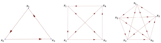
Figure 1. Directed complete graphs

We next present a flat directed graph.

Example 4.2.

For $n\geq 4$, we consider the unweighted directed cycle with $n$ vertices, denoted by $C_{n}$ (see Figure 2). Then $\kappa(C_{n})=0$. For $i=1,\dots,n$, let $x_{i}$ be vertexes as in Figure 2. It suffices to show that $\kappa(x_{1},x_{2})=0$. Since this graph is $1$-regular, (2.9) implies

$$\nu^{\varepsilon}_{x_{1}}(x_{i})=\begin{cases}1-\varepsilon&\text{if $i=1$},\\ \cfrac{\varepsilon}{2}&\text{if $i=2$ or $n$},\\ 0&\text{otherwise},\end{cases}\quad\nu^{\varepsilon}_{x_{2}}(x_{i})=\begin{cases}1-\varepsilon&\text{if $i=2$},\\ \cfrac{\varepsilon}{2}&\text{if $i=1$ or $3$},\\ 0&\text{otherwise}.\end{cases}$$

We define a coupling $\pi$ of $(\nu^{\varepsilon}_{x_{1}},\nu^{\varepsilon}_{x_{2}})$ as

$$\pi(z,w):=\begin{cases}1-\varepsilon&\text{if $(z,w)=(x_{1},x_{2})$},\\ \cfrac{\varepsilon}{2}&\text{if $(z,w)=(x_{2},x_{3})$ or $(x_{n},x_{1})$},\\ 0&\text{otherwise}.\end{cases}$$

By using this coupling and $(\ref{eq:Wasserstein distance})$ we possess $W(\nu^{\varepsilon}_{x_{1}},\nu^{\varepsilon}_{x_{2}})\leq 1$, and thus $\kappa(x_{1},x_{2})\geq 0$. We also define a $1$-Lipschitz function $f:V\to\mathbb{R}$ as

$$f(z):=\begin{cases}1&\text{if $z=x_{2}$},\\ 0&\text{if $z=x_{1}$},\\ -1&\text{if $z=x_{n}$},\\ 2&\text{otherwise}.\end{cases}$$

Applying Proposition 2.7 to $f$ leads to $\kappa(x_{1},x_{2})\leq 0$. We obtain $\kappa(x_{1},x_{2})=0$. From (2.9), one can also deduce that for all $i=1,\dots,n$,

$$\mathcal{H}_{x_{i}}=\overleftarrow{\mathcal{H}}_{x_{i}}=-\frac{n}{2}.$$

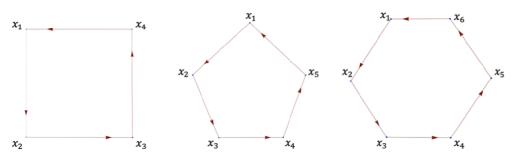
Figure 2. Directed cycles

We also provide a directed graph with negatively curved edges.

Example 4.3.

We consider the unweighted directed graph as shown in Figure 3. Then we have $\kappa(x,y)=-2$ for the vertexes $x,y$ as shown in Figure 3. We can show this estimate as follows: Since this graph is Eulerian, the formula (2.9) tells us that the two probability measures $\nu^{\varepsilon}_{x},\nu^{\varepsilon}_{y}$ are given by

$$\nu^{\varepsilon}_{x}(z)=\begin{cases}1-\varepsilon&\text{if $z=x$,}\\ \cfrac{\varepsilon}{4}&\text{if $z\in\mathcal{N}_{x}$,}\\ 0&\text{otherwise},\end{cases}\quad\nu^{\varepsilon}_{y}(z)=\begin{cases}1-\varepsilon&\text{if $z=y$,}\\ \cfrac{\varepsilon}{4}&\text{if $z\in\mathcal{N}_{y}$,}\\ 0&\text{otherwise}.\end{cases}$$

For $i=1,2,3$, let $x_{i},y_{i}$ be as in Figure 3. We define a coupling $\pi$ of $(\nu^{\varepsilon}_{x},\nu^{\varepsilon}_{y})$ by

$$\pi(z,w):=\begin{cases}1-\varepsilon&\text{if $(z,w)=(x,y)$},\\ \cfrac{\varepsilon}{4}&\text{if $(z,w)=(x_{1},y_{1})$ or $(x_{2},y_{2})$ or $(x_{3},x)$ or $(y,y_{3})$},\\ 0&\text{otherwise}.\end{cases}$$

Then one can prove $W(\nu^{\varepsilon}_{x},\nu^{\varepsilon}_{y})\leq 1+2\varepsilon$ by $(\ref{eq:Wasserstein distance})$, and hence $\kappa(x,y)\geq-2$. To check the opposite inequality, we define a function $f:\mathcal{N}_{x}\cup\mathcal{N}_{y}\to\mathbb{R}$ by

$$f(z):=\begin{cases}7&\text{if $z=y_{3}$},\\ 5&\text{if $z=y_{1}$ or $y_{2}$},\\ 4&\text{if $z=y$},\\ 3&\text{if $z=x$},\\ 2&\text{if $z=x_{1}$ or $x_{2}$},\\ 0&\text{if $z=x_{3}$},\\ \end{cases}$$

which is $1$-Lipschitz on $\mathcal{N}_{x}\cup\mathcal{N}_{y}$. We can extend $f$ to a $1$-Lipschitz function over $V$. Applying Proposition 2.7 to it, we obtain $\kappa(x,y)\leq-2$. This proves $\kappa(x,y)=-2$.

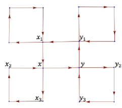
Figure 3. Directed graph with negatively curved edges

5. Products

This section is devoted to the calculation of our Ricci curvature for the weighted Cartesian product of directed graphs. We consider the weighted Cartesian product of $(V,\mu)$, and another simple, strongly connected, finite weighted directed graph $(V^{\prime},\mu^{\prime})$.

5.1. Weighted Cartesian products

We recall the notion of the weighted Cartesian product. For two parameters $\alpha,\beta>0$, the $(\alpha,\beta)$-weighted Cartesian product $(V,\mu)\square_{(\alpha,\beta)}(V^{\prime},\mu^{\prime})$ of $(V,\mu)$ and $(V^{\prime},\mu^{\prime})$ is defined as follows (cf. Subsection 2.6 in [11], Definition 2.17 in [17], and Remark 5.1 below): Its vertex set is $V\times V^{\prime}$, and its edge weight is given by

(5.1) $$\mu_{(\alpha,\beta)}(\mathbf{x},\mathbf{y}):=\beta\mu^{\prime}(x^{\prime})\mu_{xy}\,\delta_{x^{\prime}}(y^{\prime})+\alpha\mu(x)\mu^{\prime}_{x^{\prime}y^{\prime}}\,\delta_{x}(y)$$

for $\mathbf{x}=(x,x^{\prime}),\mathbf{y}=(y,y^{\prime})\in V\times V^{\prime}$, which can also be written as

$$\mu_{(\alpha,\beta)}(\mathbf{x},\mathbf{y})=\begin{cases}\beta\mu^{\prime}(x^{\prime})\mu_{xy}&\text{if $x^{\prime}=y^{\prime}$},\\ \alpha\mu(x)\mu^{\prime}_{x^{\prime}y^{\prime}}&\text{if $x=y$},\\ 0&\text{otherwise}.\end{cases}$$

Here $\mu^{\prime}(x^{\prime})$ denotes the vertex weight at $x^{\prime}$ on $(V^{\prime},\mu^{\prime})$, and we will denote by $\mu_{(\alpha,\beta)}(\mathbf{x})$ the vertex weight at $\mathbf{x}$ on $(V,\mu)\square_{(\alpha,\beta)}(V^{\prime},\mu^{\prime})$. We immediately see that $\mu_{(\alpha,\beta)}(\mathbf{x},\mathbf{x})=0$ since $(V,\mu)$ and $(V^{\prime},\mu^{\prime})$ are simple; in particular, this weighted Cartesian product is also simple. We also observe that $\mu_{(\alpha,\beta)}(\mathbf{x},\mathbf{y})>0$ if and only if either (1) $\mu^{\prime}_{x^{\prime}y^{\prime}}>0$ and $x=y$; or (2) $\mu_{xy}>0$ and $x^{\prime}=y^{\prime}$, and hence $\mathbf{x}\rightarrow\mathbf{y}$ if and only if either (1) $x^{\prime}\rightarrow y^{\prime}$ and $x=y$; or (2) $x\rightarrow y$ and $x^{\prime}=y^{\prime}$. Therefore, the strongly connectedness of $(V,\mu)$ and $(V^{\prime},\mu^{\prime})$ tells us that this weighted Cartesian product is also strongly connected. Moreover, its distance function $d_{(\alpha,\beta)}:(V\times V^{\prime})\times(V\times V^{\prime})\to[0,\infty)$ can be expressed as

(5.2) $$d_{(\alpha,\beta)}(\mathbf{x},\mathbf{y})=d(x,y)+d^{\prime}(x^{\prime},y^{\prime})$$

for the distance functions $d$ and $d^{\prime}$ on $(V,\mu)$ and $(V^{\prime},\mu^{\prime})$, respectively. In other words, $d_{(\alpha,\beta)}$ is the $l^{1}$-distance function.

Remark 5.1.

In [11], the weighted Cartesian product has been formulated as $(V,\mu)\square_{(\alpha,\beta)}(V^{\prime},\mu^{\prime})$ with $\alpha\equiv 1$ and $\beta\equiv 1$ in our notation (see Subsection 2.6 in [11]). Also, in [17], it has been done as $(V,\mu)\square_{(\alpha,\beta)}(V^{\prime},\mu^{\prime})$, which generalizes that in [11] (see Definition 2.7 in [17]). When $(V,\mu)$ is $r$-regular and $(V^{\prime},\mu^{\prime})$ is $r^{\prime}$-regular, the formulation in [17] agrees with the standard Cartesian product by taking $\alpha=1/r$ and $\beta=1/r^{\prime}$ (see Lemma 2.19 in [17]).

We now summarize some formulas on the weighted Cartesian product $(V,\mu)\square_{(\alpha,\beta)}(V^{\prime},\mu^{\prime})$ (cf. Lemma 2.18 in [17]). We denote by $P^{\prime},\mathfrak{m}^{\prime},\overleftarrow{P}^{\prime},\mathcal{P}^{\prime}$ the transition probability kernel, the Perron measure, the reverse transition probability kernel, the mean transition probability kernel on $(V^{\prime},\mu^{\prime})$, respectively. Similarly, we denote by $P_{(\alpha,\beta)},\mathfrak{m}_{(\alpha,\beta)},\overleftarrow{P}_{(\alpha,\beta)},\mathcal{P}_{(\alpha,\beta)}$ the transition probability kernel, the Perron measure, the reverse transition probability kernel, the mean transition probability kernel on $(V,\mu)\square_{(\alpha,\beta)}(V^{\prime},\mu^{\prime})$, respectively.

Lemma 5.2.

For $\mathbf{x}=(x,x^{\prime}),\mathbf{y}=(y,y^{\prime})\in V\times V^{\prime}$, we have

(5.3) $$\mu_{(\alpha,\beta)}(\mathbf{x}) =(\alpha+\beta)\mu(x)\mu^{\prime}(x^{\prime}),$$

(5.4) $$P_{(\alpha,\beta)}(\mathbf{x},\mathbf{y}) =\frac{\beta}{\alpha+\beta}P(x,y)\delta_{x^{\prime}}(y^{\prime})+\frac{\alpha}{\alpha+\beta}P^{\prime}(x^{\prime},y^{\prime})\delta_{x}(y),$$

(5.5) $$\mathfrak{m}_{(\alpha,\beta)}(\mathbf{x}) =\mathfrak{m}(x)\mathfrak{m}^{\prime}(x^{\prime}),$$

(5.6) $$\overleftarrow{P}_{(\alpha,\beta)}(\mathbf{x},\mathbf{y}) =\frac{\beta}{\alpha+\beta}\overleftarrow{P}(x,y)\delta_{x^{\prime}}(y^{\prime})+\frac{\alpha}{\alpha+\beta}\overleftarrow{P}^{\prime}(x^{\prime},y^{\prime})\delta_{x}(y),$$

(5.7) $$\mathcal{P}_{(\alpha,\beta)}(\mathbf{x},\mathbf{y}) =\frac{\beta}{\alpha+\beta}\mathcal{P}(x,y)\delta_{x^{\prime}}(y^{\prime})+\frac{\alpha}{\alpha+\beta}\mathcal{P}^{\prime}(x^{\prime},y^{\prime})\delta_{x}(y).$$

Proof.

We begin with the proof of (5.3). By (5.1), it holds that

$$\mu_{(\alpha,\beta)}(\mathbf{x}) =\sum_{\mathbf{z}\in V\times V^{\prime}}\mu_{(\alpha,\beta)}(\mathbf{x},\mathbf{z})=\sum_{z\in V,z^{\prime}\in V^{\prime}}\left(\beta\mu^{\prime}(x^{\prime})\mu_{xz}\,\delta_{x^{\prime}}(z^{\prime})+\alpha\mu(x)\mu^{\prime}_{x^{\prime}z^{\prime}}\,\delta_{x}(z)\right)$$

$$=\beta\mu^{\prime}(x^{\prime})\sum_{z\in V}\mu_{xz}+\alpha\mu(x)\sum_{z^{\prime}\in V^{\prime}}\mu^{\prime}_{x^{\prime}z^{\prime}}=(\beta+\alpha)\mu(x)\mu^{\prime}(x^{\prime})$$

for $\mathbf{z}=(z,z^{\prime})\in V\times V^{\prime}$, and hence (5.3). Further, (5.4) directly follows from (5.1), (5.3).

We next show (5.5). We define a probability measure $\widetilde{\mathfrak{m}}:V\times V^{\prime}\to(0,1]$ by

$$\widetilde{\mathfrak{m}}(\mathbf{z})=\mathfrak{m}(z)\mathfrak{m}^{\prime}(z^{\prime}).$$

In virtue of the uniqueness of the Perron measure, it suffices to verify

(5.8) $$\widetilde{\mathfrak{m}}(\mathbf{x})=\sum_{\mathbf{z}\in V\times V^{\prime}}\widetilde{\mathfrak{m}}(\mathbf{z})P_{(\alpha,\beta)}(\mathbf{z},\mathbf{x}).$$

Using (5.4), we can calculate the right hand side of (5.8) as follows:

$$\quad\,\,\sum_{\mathbf{z}\in V\times V^{\prime}}\widetilde{\mathfrak{m}}(\mathbf{z})P_{(\alpha,\beta)}(\mathbf{z},\mathbf{x})$$

$$=\sum_{z\in V,z^{\prime}\in V^{\prime}}\mathfrak{m}(z)\mathfrak{m}^{\prime}(z^{\prime})\left(\frac{\beta}{\alpha+\beta}P(z,x)\delta_{x^{\prime}}(z^{\prime})+\frac{\alpha}{\alpha+\beta}P^{\prime}(z^{\prime},x^{\prime})\delta_{x}(z)\right)$$

$$=\frac{\beta}{\alpha+\beta}\mathfrak{m}^{\prime}(x^{\prime})\sum_{z\in V}\mathfrak{m}(z)P(z,x)+\frac{\alpha}{\alpha+\beta}\mathfrak{m}(x)\sum_{z^{\prime}\in V^{\prime}}\mathfrak{m}^{\prime}(z^{\prime})P^{\prime}(z^{\prime},x^{\prime})$$

(5.9) $$=\frac{\beta}{\alpha+\beta}\mathfrak{m}^{\prime}(x^{\prime})\mathfrak{m}(x)+\frac{\alpha}{\alpha+\beta}\mathfrak{m}(x)\mathfrak{m}^{\prime}(x^{\prime})=\mathfrak{m}(x)\mathfrak{m}^{\prime}(x^{\prime})=\widetilde{\mathfrak{m}}(\mathbf{x}),$$

and thus (5.8). Here we used the fact that $\mathfrak{m}$ and $\mathfrak{m}^{\prime}$ are the Perron measures in (5.9).

Let us prove (5.6). Combining (5.4) and (5.5), we have

$$\overleftarrow{P}_{(\alpha,\beta)}(\mathbf{x},\mathbf{y}) =\frac{\mathfrak{m}_{(\alpha,\beta)}(\mathbf{y})}{\mathfrak{m}_{(\alpha,\beta)}(\mathbf{x})}P_{(\alpha,\beta)}(\mathbf{y},\mathbf{x})$$

$$=\frac{\mathfrak{m}(y)\mathfrak{m}^{\prime}(y^{\prime})}{\mathfrak{m}(x)\mathfrak{m}^{\prime}(x^{\prime})}\left(\frac{\beta}{\alpha+\beta}P(y,x)\delta_{y^{\prime}}(x^{\prime})+\frac{\alpha}{\alpha+\beta}P^{\prime}(y^{\prime},x^{\prime})\delta_{y}(x)\right)$$

$$=\frac{\beta}{\alpha+\beta}\overleftarrow{P}(x,y)\frac{\mathfrak{m}^{\prime}(y^{\prime})}{\mathfrak{m}^{\prime}(x^{\prime})}\delta_{y^{\prime}}(x^{\prime})+\frac{\alpha}{\alpha+\beta}\overleftarrow{P}^{\prime}(x^{\prime},y^{\prime})\frac{\mathfrak{m}(y)}{\mathfrak{m}(x)}\delta_{y}(x)$$

$$=\frac{\beta}{\alpha+\beta}\overleftarrow{P}(x,y)\delta_{x^{\prime}}(y^{\prime})+\frac{\alpha}{\alpha+\beta}\overleftarrow{P}^{\prime}(x^{\prime},y^{\prime})\delta_{x}(y).$$

This proves (5.6). The last one (5.7) is an immediate consequence of (5.4) and (5.6). $\Box$

Let $\varepsilon\in[0,1]$ and $\mathbf{x}=(x,x^{\prime})\in V\times V^{\prime}$. We next examine a probability measure $\nu_{(\alpha,\beta),\mathbf{x}}^{\varepsilon}:V\times V^{\prime}\to[0,1]$ on $(V,\mu)\square_{(\alpha,\beta)}(V^{\prime},\mu^{\prime})$ defined as (3.1). Let $(\nu^{\varepsilon}_{x^{\prime}})^{\prime}:V^{\prime}\to[0,1]$ stand for a probability measure over $(V^{\prime},\mu^{\prime})$ defined as (3.1).

Lemma 5.3.

Let $\varepsilon\in[0,1]$ and $\mathbf{x}=(x,x^{\prime})\in V\times V^{\prime}$. For every $\mathbf{z}=(z,z^{\prime})\in V\times V^{\prime}$,

$$\nu_{(\alpha,\beta),\mathbf{x}}^{\varepsilon}(\mathbf{z})=\frac{\beta}{\alpha+\beta}\nu^{\varepsilon}_{x|x^{\prime}}(\mathbf{z})+\frac{\alpha}{\alpha+\beta}(\nu^{\varepsilon}_{x^{\prime}|x})^{\prime}(\mathbf{z}),$$

where two probability measures $\nu^{\varepsilon}_{x|x^{\prime}},(\nu^{\varepsilon}_{x^{\prime}|x})^{\prime}:(V\times V^{\prime})\times(V\times V^{\prime})\to[0,1]$ are defined as

(5.10) $$\nu^{\varepsilon}_{x|x^{\prime}}(\mathbf{z}):=\nu^{\varepsilon}_{x}(z)\delta_{x^{\prime}}(z^{\prime}),\quad(\nu^{\varepsilon}_{x^{\prime}|x})^{\prime}(\mathbf{z}):=(\nu^{\varepsilon}_{x^{\prime}})^{\prime}(z^{\prime})\delta_{x}(z).$$

Proof.

In view of the expression (3.2), the formula (5.7) implies

$$\nu_{(\alpha,\beta),\mathbf{x}}^{\varepsilon}(\mathbf{z}) =(1-\varepsilon)\delta_{\mathbf{x}}(\mathbf{z})+\varepsilon\,\mathcal{P}_{(\alpha,\beta)}(\mathbf{x},\mathbf{z})$$

$$=(1-\varepsilon)\delta_{x}(z)\delta_{x^{\prime}}(z^{\prime})+\varepsilon\,\left(\frac{\beta}{\alpha+\beta}\mathcal{P}(x,z)\delta_{x^{\prime}}(z^{\prime})+\frac{\alpha}{\alpha+\beta}\mathcal{P}^{\prime}(x^{\prime},z^{\prime})\delta_{x}(z)\right)$$

$$=\frac{\beta}{\alpha+\beta}((1-\varepsilon)\delta_{x}(z)+\varepsilon\,\mathcal{P}(x,z))\delta_{x^{\prime}}(z^{\prime})$$

$$\quad+\frac{\alpha}{\alpha+\beta}((1-\varepsilon)\delta_{x^{\prime}}(z^{\prime})+\varepsilon\,\mathcal{P}^{\prime}(x^{\prime},z^{\prime}))\delta_{x}(z)$$

$$=\frac{\beta}{\alpha+\beta}\nu^{\varepsilon}_{x|x^{\prime}}(\mathbf{z})+\frac{\alpha}{\alpha+\beta}(\nu^{\varepsilon}_{x^{\prime}|x})^{\prime}(\mathbf{z}).$$

This completes the proof. $\Box$

We further investigate the Laplacian. Let $\mathcal{L}^{\prime}$ and $\mathcal{L}_{(\alpha,\beta)}$ be the Laplacian over $(V^{\prime},\mu^{\prime})$ and $(V,\mu)\square_{(\alpha,\beta)}(V^{\prime},\mu^{\prime})$, respectively.

Lemma 5.4.

For $f:V\to\mathbb{R}$ and $f^{\prime}:V^{\prime}\to\mathbb{R}$, we define a function $\mathbf{f}:V\times V^{\prime}\to\mathbb{R}$ by

$$\mathbf{f}(\mathbf{x}):=f(x)+f^{\prime}(x^{\prime})$$

for $\mathbf{x}=(x,x^{\prime})\in V\times V^{\prime}$. Then for every $\mathbf{x}=(x,x^{\prime})\in V\times V^{\prime}$ we have

$$\mathcal{L}_{(\alpha,\beta)}\mathbf{f}(\mathbf{x})=\frac{\beta}{\alpha+\beta}\mathcal{L}f(x)+\frac{\alpha}{\alpha+\beta}\mathcal{L}^{\prime}f^{\prime}(x^{\prime}).$$

Proof.

The formula (5.7) yields

$$\quad\,\,\sum_{\mathbf{y}\in V\times V^{\prime}}\mathcal{P}_{(\alpha,\beta)}(\mathbf{x},\mathbf{y})\mathbf{f}(\mathbf{y})$$

$$=\sum_{y\in V,y^{\prime}\in V^{\prime}}\left(\frac{\beta}{\alpha+\beta}\mathcal{P}(x,y)\delta_{x^{\prime}}(y^{\prime})+\frac{\alpha}{\alpha+\beta}\mathcal{P}^{\prime}(x^{\prime},y^{\prime})\delta_{x}(y)\right)(f(y)+f^{\prime}(y^{\prime}))$$

$$=\frac{\beta}{\alpha+\beta}\sum_{y\in V}\mathcal{P}(x,y)(f(y)+f^{\prime}(x^{\prime}))+\frac{\alpha}{\alpha+\beta}\sum_{y^{\prime}\in V^{\prime}}\mathcal{P}^{\prime}(x^{\prime},y^{\prime})(f(x)+f^{\prime}(y^{\prime}))$$

$$=\frac{\alpha}{\alpha+\beta}f(x)+\frac{\beta}{\alpha+\beta}f^{\prime}(x^{\prime})+\frac{\beta}{\alpha+\beta}\sum_{y\in V}\mathcal{P}(x,y)f(y)+\frac{\alpha}{\alpha+\beta}\sum_{y^{\prime}\in V^{\prime}}\mathcal{P}^{\prime}(x^{\prime},y^{\prime})f^{\prime}(y^{\prime}).$$

The above equality implies

$$\mathcal{L}_{(\alpha,\beta)}\mathbf{f}(\mathbf{x}) =\mathbf{f}(\mathbf{x})-\sum_{\mathbf{y}\in V\times V^{\prime}}\mathcal{P}_{(\alpha,\beta)}(\mathbf{x},\mathbf{y})\mathbf{f}(\mathbf{y})$$

$$=\frac{\beta}{\alpha+\beta}\left(f(x)-\sum_{y\in V}\mathcal{P}(x,y)f(y)\right)+\frac{\alpha}{\alpha+\beta}\left(f^{\prime}(x^{\prime})-\sum_{y^{\prime}\in V}\mathcal{P}^{\prime}(x^{\prime},y^{\prime})f^{\prime}(y^{\prime})\right)$$

$$=\frac{\beta}{\alpha+\beta}\mathcal{L}f(x)+\frac{\alpha}{\alpha+\beta}\mathcal{L}^{\prime}f^{\prime}(x^{\prime}).$$

We arrive at the desired formula. $\Box$

We end this subsection with formulas for asymptotic mean curvature. Let $\mathbf{x}=(x,x^{\prime}),\mathbf{y}=(y,y^{\prime})\in V\times V^{\prime}$. We denote by $\mathcal{H}^{\prime}_{x^{\prime}},\overleftarrow{\mathcal{H}}^{\prime}_{x^{\prime}},\mathcal{H}^{\prime}(x^{\prime},y^{\prime})$ the asymptotic mean curvature around $x^{\prime}$, the reverse asymptotic mean curvature, the mixed asymptotic mean curvature over $(V^{\prime},\mu^{\prime})$, respectively. Also, let $\mathcal{H}_{(\alpha,\beta),\mathbf{x}},\overleftarrow{\mathcal{H}}_{(\alpha,\beta),\mathbf{x}},\mathcal{H}_{(\alpha,\beta)}(\mathbf{x},\mathbf{y})$ stand for the asymptotic mean curvature around $\mathbf{x}$, the reverse asymptotic mean curvature, the mixed asymptotic mean curvature over $(V,\mu)\square_{(\alpha,\beta)}(V^{\prime},\mu^{\prime})$, respectively.

Proposition 5.5.

For $\mathbf{x}=(x,x^{\prime}),\mathbf{y}=(y,y^{\prime})\in V\times V^{\prime}$, we have

$$\mathcal{H}_{(\alpha,\beta),\mathbf{x}} =\frac{\beta}{\alpha+\beta}\mathcal{H}_{x}+\frac{\alpha}{\alpha+\beta}\mathcal{H}^{\prime}_{x^{\prime}},$$

$$\overleftarrow{\mathcal{H}}_{(\alpha,\beta),\mathbf{x}} =\frac{\beta}{\alpha+\beta}\overleftarrow{\mathcal{H}}_{x}+\frac{\alpha}{\alpha+\beta}\overleftarrow{\mathcal{H}}^{\prime}_{x^{\prime}},$$

$$\mathcal{H}_{(\alpha,\beta)}(\mathbf{x},\mathbf{y}) =\frac{\beta}{\alpha+\beta}\mathcal{H}(x,y)+\frac{\alpha}{\alpha+\beta}\mathcal{H}^{\prime}(x^{\prime},y^{\prime}).$$

Proof.

These formulas directly follow from (5.2) and Lemma 5.4. $\Box$

5.2. Ricci curvature of weighted Cartesian products

We calculate the Ricci curvature of the $(\alpha,\beta)$-weighted Cartesian product $(V,\mu)\square_{(\alpha,\beta)}(V^{\prime},\mu^{\prime})$ introduced in the above subsection. For $x^{\prime},y^{\prime}\in V^{\prime}$ with $x^{\prime}\neq y^{\prime}$, let $\kappa^{\prime}(x^{\prime},y^{\prime})$ denote the Ricci curvature over $(V^{\prime},\mu^{\prime})$ defined as Definition 3.6. For $\mathbf{x},\mathbf{y}\in V\times V^{\prime}$ with $\mathbf{x}\neq\mathbf{y}$, we also denote by $\kappa_{(\alpha,\beta)}(\mathbf{x},\mathbf{y})$ the Ricci curvature over $(V,\mu)\square_{(\alpha,\beta)}(V^{\prime},\mu^{\prime})$. We obtain the following (cf. Theorem 3.1 in [24]):

Theorem 5.6.

Let $\mathbf{x}=(x,x^{\prime}),\mathbf{y}=(y,y^{\prime})\in V\times V^{\prime}$ with $\mathbf{x}\neq\mathbf{y}$. Then we have the following:

1. If $x\neq y$ and $x^{\prime}\neq y^{\prime}$, then

   (5.11) $$\kappa_{(\alpha,\beta)}(\mathbf{x},\mathbf{y})=\frac{\beta}{\alpha+\beta}\frac{d(x,y)}{d(x,y)+d^{\prime}(x^{\prime},y^{\prime})}\kappa(x,y)+\frac{\alpha}{\alpha+\beta}\frac{d^{\prime}(x^{\prime},y^{\prime})}{d(x,y)+d^{\prime}(x^{\prime},y^{\prime})}\kappa^{\prime}(x^{\prime},y^{\prime});$$

2. if $x\neq y$ and $x^{\prime}=y^{\prime}$, then

   (5.12) $$\kappa_{(\alpha,\beta)}(\mathbf{x},\mathbf{y})=\frac{\beta}{\alpha+\beta}\kappa(x,y);$$

3. if $x=y$ and $x^{\prime}\neq y^{\prime}$, then

   (5.13) $$\kappa_{(\alpha,\beta)}(\mathbf{x},\mathbf{y})=\frac{\alpha}{\alpha+\beta}\kappa^{\prime}(x^{\prime},y^{\prime}).$$

Proof.

We only prove the formula (5.11). The others (5.12) and (5.13) can be proved by the same argument as in the proof of (5.11), and more easily. We assume $x\neq y$ and $x^{\prime}\neq y^{\prime}$.

We first show that

(5.14) $$\kappa_{(\alpha,\beta)}(\mathbf{x},\mathbf{y})\geq\frac{\beta}{\alpha+\beta}\frac{d(x,y)}{d(x,y)+d^{\prime}(x^{\prime},y^{\prime})}\kappa(x,y)+\frac{\alpha}{\alpha+\beta}\frac{d^{\prime}(x^{\prime},y^{\prime})}{d(x,y)+d^{\prime}(x^{\prime},y^{\prime})}\kappa^{\prime}(x^{\prime},y^{\prime}).$$

In order to obtain the lower bound of $\kappa_{(\alpha,\beta)}(\mathbf{x},\mathbf{y})$, we estimate the Wasserstein distance from above. Proposition 2.6 and Lemma 5.3 yield that for every $\varepsilon\in(0,1]$,

(5.15) $$W(\nu_{(\alpha,\beta),\mathbf{x}}^{\varepsilon},\nu_{(\alpha,\beta),\mathbf{y}}^{\varepsilon}) =W\left(\frac{\beta}{\alpha+\beta}\nu^{\varepsilon}_{x|x^{\prime}}+\frac{\alpha}{\alpha+\beta}(\nu^{\varepsilon}_{x^{\prime}|x})^{\prime},\frac{\beta}{\alpha+\beta}\nu^{\varepsilon}_{y|y^{\prime}}+\frac{\alpha}{\alpha+\beta}(\nu^{\varepsilon}_{y^{\prime}|y})^{\prime}\right)$$

$$\leq\frac{\beta}{\alpha+\beta}W(\nu^{\varepsilon}_{x|x^{\prime}},\nu^{\varepsilon}_{y|y^{\prime}})+\frac{\alpha}{\alpha+\beta}W((\nu^{\varepsilon}_{x^{\prime}|x})^{\prime},(\nu^{\varepsilon}_{y^{\prime}|y})^{\prime}),$$

where the probability measures $\nu^{\varepsilon}_{x|x^{\prime}},\nu^{\varepsilon}_{y|y^{\prime}},(\nu^{\varepsilon}_{x^{\prime}|x})^{\prime},(\nu^{\varepsilon}_{y^{\prime}|y})^{\prime}$ are defined as (5.10). Let us estimate $W(\nu^{\varepsilon}_{x|x^{\prime}},\nu^{\varepsilon}_{y|y^{\prime}})$ from above. To do so, we fix an optimal coupling $\pi_{xy}:V\times V\to[0,1]$ of $(\nu_{x}^{\varepsilon},\nu_{y}^{\varepsilon})$, and define a probability measure $\pi:(V\times V^{\prime})\times(V\times V^{\prime})\to[0,1]$ by

$$\pi(\mathbf{z},\mathbf{w}):=\pi_{xy}(z,w)\delta_{x^{\prime}}(z^{\prime})\delta_{y^{\prime}}(w^{\prime}).$$

We can check that $\pi$ is a coupling of $(\nu^{\varepsilon}_{x|x^{\prime}},\nu^{\varepsilon}_{y|y^{\prime}})$. From (5.2) we deduce

(5.16) $$W(\nu^{\varepsilon}_{x|x^{\prime}},\nu^{\varepsilon}_{y|y^{\prime}}) \leq\sum_{\mathbf{z},\mathbf{w}\in V\times V^{\prime}}d_{(\alpha,\beta)}(\mathbf{z},\mathbf{w})\pi(\mathbf{z},\mathbf{w})$$

$$=\sum_{z,w\in V}\sum_{z^{\prime},w^{\prime}\in V^{\prime}}(d(z,w)+d^{\prime}(z^{\prime},w^{\prime}))\pi_{xy}(z,w)\delta_{x^{\prime}}(z^{\prime})\delta_{y^{\prime}}(w^{\prime})$$

$$=\sum_{z,w\in V}(d(z,w)+d^{\prime}(x^{\prime},y^{\prime}))\pi_{xy}(z,w)=W(\nu_{x}^{\varepsilon},\nu_{y}^{\varepsilon})+d^{\prime}(x^{\prime},y^{\prime}).$$

We can also prove

(5.17) $$W((\nu^{\varepsilon}_{x^{\prime}|x})^{\prime},(\nu^{\varepsilon}_{y^{\prime}|y})^{\prime})\leq d(x,y)+W((\nu_{x^{\prime}}^{\varepsilon})^{\prime},(\nu_{y^{\prime}}^{\varepsilon})^{\prime})$$

by considering a coupling $\pi^{\prime}:(V\times V^{\prime})\times(V\times V^{\prime})\to[0,1]$ of $((\nu^{\varepsilon}_{x^{\prime}|x})^{\prime},(\nu^{\varepsilon}_{y^{\prime}|y})^{\prime})$ defined as

$$\pi^{\prime}(\mathbf{z},\mathbf{w}):=\pi^{\prime}_{x^{\prime}y^{\prime}}(z^{\prime},w^{\prime})\delta_{x}(z)\delta_{y}(w)$$

for a fixed optimal coupling $\pi^{\prime}_{x^{\prime}y^{\prime}}:V^{\prime}\times V^{\prime}\to[0,1]$ of $((\nu_{x^{\prime}}^{\varepsilon})^{\prime},(\nu_{y^{\prime}}^{\varepsilon})^{\prime})$, and by applying the same calculation as in (5.16). Substituting (5.16) and (5.17) into (5.15), we arrive at

(5.18) $$W(\nu_{(\alpha,\beta),\mathbf{x}}^{\varepsilon},\nu_{(\alpha,\beta),\mathbf{y}}^{\varepsilon}) \leq\frac{\beta}{\alpha+\beta}\left(W(\nu_{x}^{\varepsilon},\nu_{y}^{\varepsilon})+d^{\prime}(x^{\prime},y^{\prime})\right)$$

$$\quad+\frac{\alpha}{\alpha+\beta}\left(d(x,y)+W((\nu_{x^{\prime}}^{\varepsilon})^{\prime},(\nu_{y^{\prime}}^{\varepsilon})^{\prime})\right).$$

Since $x\neq y$ and $x^{\prime}\neq y^{\prime}$, we can rewrite (5.18) as

$$1-\frac{W(\nu_{(\alpha,\beta),\mathbf{x}}^{\varepsilon},\nu_{(\alpha,\beta)\mathbf{y}}^{\varepsilon})}{d_{(\alpha,\beta)}(\mathbf{x},\mathbf{y})} \geq\frac{\beta}{\alpha+\beta}\frac{d(x,y)}{d_{(\alpha,\beta)}(\mathbf{x},\mathbf{y})}\left(1-\frac{W(\nu_{x}^{\varepsilon},\nu_{y}^{\varepsilon})}{d(x,y)}\right)$$

$$\quad+\frac{\alpha}{\alpha+\beta}\frac{d^{\prime}(x^{\prime},y^{\prime})}{d_{(\alpha,\beta)}(\mathbf{x},\mathbf{y})}\left(1-\frac{W((\nu_{x^{\prime}}^{\varepsilon})^{\prime},(\nu_{y^{\prime}}^{\varepsilon})^{\prime})}{d^{\prime}(x^{\prime},y^{\prime})}\right).$$

Dividing its both sides by $\varepsilon$, we obtain the relation for $\kappa_{\varepsilon}$ defined (3.4). Moreover, letting $\varepsilon\to 0$, we conclude (5.14) from (5.2).

We next prove the opposite inequality of (5.14). Take functions $f:V\to\mathbb{R}$ and $f^{\prime}:V^{\prime}\to\mathbb{R}$ with $\nabla_{xy}f=1$ and $\nabla^{\prime}_{x^{\prime}y^{\prime}}f^{\prime}=1$, where $\nabla_{xy}$ and $\nabla^{\prime}_{x^{\prime}y^{\prime}}$ are the gradient operators over $(V,\mu)$ and $(V^{\prime},\mu^{\prime})$ defined as (3.9), respectively. We define a function $\mathbf{f}:V\times V^{\prime}\to\mathbb{R}$ by

$$\mathbf{f}(\mathbf{x}):=f(x)+f^{\prime}(x^{\prime}).$$

Then we deduce $\nabla_{(\alpha,\beta),\mathbf{x}\mathbf{y}}\mathbf{f}=1$ from (5.2), where $\nabla_{(\alpha,\beta),\mathbf{x}\mathbf{y}}$ denotes the gradient operator over $(V,\mu)\square_{(\alpha,\beta)}(V^{\prime},\mu^{\prime})$. Hence, by Theorem 3.10 and Lemma 5.4, we have

$$\kappa_{(\alpha,\beta)}(\mathbf{x},\mathbf{y}) \leq\nabla_{(\alpha,\beta),\mathbf{x}\mathbf{y}}\mathcal{L}_{(\alpha,\beta)}\mathbf{f}=\frac{\mathcal{L}_{(\alpha,\beta)}\mathbf{f}(\mathbf{y})-\mathcal{L}_{(\alpha,\beta)}\mathbf{f}(\mathbf{x})}{d_{(\alpha,\beta)}(\mathbf{x},\mathbf{y})}$$

$$=\frac{1}{d_{(\alpha,\beta)}(\mathbf{x},\mathbf{y})}\left(\frac{\beta}{\alpha+\beta}(\mathcal{L}f(y)-\mathcal{L}f(x))+\frac{\alpha}{\alpha+\beta}(\mathcal{L}^{\prime}f^{\prime}(y^{\prime})-\mathcal{L}^{\prime}f^{\prime}(x^{\prime}))\right)$$

$$=\frac{\beta}{\alpha+\beta}\frac{d(x,y)}{d_{(\alpha,\beta)}(\mathbf{x},\mathbf{y})}\nabla_{xy}\mathcal{L}f+\frac{\alpha}{\alpha+\beta}\frac{d^{\prime}(x^{\prime},y^{\prime})}{d_{(\alpha,\beta)}(\mathbf{x},\mathbf{y})}\nabla^{\prime}_{x^{\prime}y^{\prime}}\mathcal{L}^{\prime}f^{\prime}.$$

Since the functions $f$ and $f^{\prime}$ are arbitrary, we conclude the opposite one by using Theorem 3.10 again. Thus we complete the proof. $\Box$

Remark 5.7.

Lin-Lu-Yau [24] have proved (5.12) and (5.13) when $(V,\mu)$ is undirected $r$-regular, $(V^{\prime},\mu^{\prime})$ is undirected $r^{\prime}$-regular, $\alpha=1/r,\beta=1/r^{\prime}$ and $\mathbf{x}\rightarrow\mathbf{y}$ (see Theorem 3.1 in [24]). Our method of the proof of (5.14) is based on that of Theorem 3.1 in [24] (see Claim 1 in [24]). On the other hand, for the proof of the opposite one, their method seems not to work in our setting due to the lack of symmetry of the distance function (see Claim 2 in [24]). Our method via Theorem 3.10 seems to be new and more clear.

The formulas (5.11), (5.12), (5.13) also hold for simple, connected, locally finite, infinite weighted undirected graphs, whose proofs are identical.

6. Estimates

In the present subsection, we discuss several upper and lower bounds of our Ricci curvature.

6.1. Lower bounds

For $x,y\in V$ with $x\neq y$, we set

$$\mathcal{D}(x,y):=\max\left\{d(x,y),d(y,x)\right\}.$$

We first study a lower bound of our Ricci curvature (cf. Theorems 2 and 5 in [20]).

Proposition 6.1.

For $x,y\in V$ with $x\neq y$, we have

(6.1) $$\kappa(x,y)\geq -\frac{2\mathcal{D}(x,y)}{d(x,y)}\,\left(1-\mathcal{P}(x,y)-\mathcal{P}(y,x)\right)_{+}+\frac{1}{d(x,y)}\left(d(x,y)+\mathcal{D}(x,y)-\mathcal{H}(y,x)\right)$$

$$-\frac{\mathcal{D}(x,y)-d(y,x)}{d(x,y)}\,\left(\mathcal{P}(x,y)+\mathcal{P}(y,x)\right),$$

where $(\cdot)_{+}$ denotes its positive part. Moreover, if $(x,y)\in E$, then we have

(6.2) $$\kappa(x,y)\geq-2d(y,x)\,\left(1-\mathcal{P}(x,y)-\mathcal{P}(y,x)\right)_{+}+\left(1+d(y,x)-\mathcal{H}(y,x)\right).$$

Proof.

Jost-Liu [20] shown (6.2) in the undirected case, whose primitive version has been established by Lin-Yau [25] (see Theorem 5 in [20], and also Proposition 1.5 in [25], Theorem 2 in [20]). We will calculate along the line of the proof of Theorem 2 in [20].

In view of Lemma 3.2, it suffices to prove that $\kappa_{1}(x,y)$ is bounded from below by the right hand side of (6.2). To do so, let us estimate $W(\nu^{1}_{x},\nu^{1}_{y})$ from above. Note that $\nu^{1}_{x}(z)=\mathcal{P}(x,z)$ and $\nu^{1}_{y}(z)=\mathcal{P}(y,z)$ for all $z\in V$. From Proposition 2.7 we deduce

$$W(\nu^{1}_{x},\nu^{1}_{y}) =\sup_{f\in\mathrm{Lip}_{1}(V)}\sum_{z\in V}f(z)(\nu_{y}^{1}(z)-\nu_{x}^{1}(z))$$

$$=\sup_{f\in\mathrm{Lip}_{1}(V)}\Biggl{\{}\Biggl{(}\sum_{z\in V\setminus\{x\}}\left(f(z)-f(y)\right)\mathcal{P}(y,z)\Biggl{)}-\Biggl{(}\sum_{z\in V\setminus\{y\}}\left(f(z)-f(x)\right)\mathcal{P}(x,z)\Biggl{)}$$

$$\qquad\qquad\qquad\qquad\qquad\qquad\qquad\qquad+\left(f(y)-f(x)\right)\left(1-\mathcal{P}(x,y)-\mathcal{P}(y,x)\right)\Biggl{\}}.$$

For any $f\in\mathrm{Lip}_{1}(V)$ we have

$$f(z)-f(y)\leq d(y,z),\quad f(z)-f(x)\geq-d(z,x),\quad|f(y)-f(x)|\leq\mathcal{D}(x,y),$$

and hence

$$W(\nu^{1}_{x},\nu^{1}_{y}) \leq\sum_{z\in V\setminus\{x\}}d(y,z)\mathcal{P}(y,z)+\sum_{z\in V\setminus\{y\}}d(z,x)\mathcal{P}(x,z)$$

$$\qquad\qquad\qquad\qquad\qquad\,\,+\mathcal{D}(x,y)\,\left|1-\mathcal{P}(x,y)-\mathcal{P}(y,x)\right|$$

$$=\left(-\mathcal{H}_{y}-d(y,x)\mathcal{P}(y,x)\right)+\left(-\overleftarrow{\mathcal{H}}_{x}-d(y,x)\mathcal{P}(x,y)\right)$$

$$\quad+\mathcal{D}(x,y)\,\left(2\left(1-\mathcal{P}(x,y)-\mathcal{P}(y,x)\right)_{+}-\left(1-\mathcal{P}(x,y)-\mathcal{P}(y,x)\right)\right)$$

$$=\mathcal{H}(y,x)-d(y,x)\,\left(\mathcal{P}(x,y)+\mathcal{P}(y,x)\right)$$

$$\quad+\mathcal{D}(x,y)\,\left(2\left(1-\mathcal{P}(x,y)-\mathcal{P}(y,x)\right)_{+}-\left(1-\mathcal{P}(x,y)-\mathcal{P}(y,x)\right)\right)$$

$$=2\mathcal{D}(x,y)\,\left(1-\mathcal{P}(x,y)-\mathcal{P}(y,x)\right)_{+}-\left(\mathcal{D}(x,y)-\mathcal{H}(y,x)\right)$$

$$\quad+\left(\mathcal{D}(x,y)-d(y,x)\right)\,\left(\mathcal{P}(x,y)+\mathcal{P}(y,x)\right),$$

here we used (3.6), (3.7). This proves (6.1).

When $(x,y)\in E$, we have $d(x,y)=1$. Furthermore,

$$\mathcal{D}(x,y)=\max\left\{d(x,y),d(y,x)\right\}=\max\left\{1,d(y,x)\right\}=d(y,x)$$

since $d(y,x)\geq 1$. Substituting these equalities into (6.1), we see that the first term in the right hand of (6.1) becomes that of (6.2), the second term also does, and the third term vanishes. Thus we obtain (6.2). $\Box$

Remark 6.2.

In the undirected case, under the same setting as in Proposition 6.1, we have $d(y,x)=1$ and $\mathcal{H}(x,y)=2$. In particular, the second term of the right hand side of (6.2) vanishes, and hence its right hand side coincides with that of Theorem 5 in [20].

For regular graphs, we derive an another lower bound in terms of the inscribed radius instead of the asymptotic mean curvature (cf. Theorem 3 in [20]).

Proposition 6.3.

For $r\geq 1$, let $(V,\mu)$ be an $r$-regular graph. Then for all edge $(x,y)\in E$,

$$\kappa(x,y)\geq\frac{1-r}{2r}-\sum_{z\in N_{x}\setminus\overleftarrow{N}_{y}}\frac{\operatorname{InRad}_{z}V}{2r},$$

where $N_{x}$ and $\overleftarrow{N}_{y}$ are defined as $(\ref{eq:neighborhoods})$, and $\operatorname{InRad}_{z}V$ is done as $(\ref{eq:inscribed radius})$.

Proof.

We take a coupling between $\nu^{\varepsilon}_{x}$ and $\nu^{\varepsilon}_{y}$. Our transfer plan moving $\nu^{\varepsilon}_{x}$ to $\nu^{\varepsilon}_{y}$ should be as follows:

1. Move the mass of $1-\varepsilon$ from $x$ to $y$. The distance is $1$;

2. Move the mass of $\varepsilon/2r$ from $y$ to a fixed $y_{0}\in N_{y}$, and move the mass of $\varepsilon/2r$ from a fixed $x_{0}\in\overleftarrow{N}_{x}$ to $x$. These distances are $1$;

3. Move the mass of $\varepsilon/2r$ to itself at $N_{x}\cap\overleftarrow{N}_{y}$;

4. Move the mass of $\varepsilon/2r$ from a vertex in $\overleftarrow{N}_{x}\setminus\left\{x_{0}\right\}$ to a vertex in $N_{y}\setminus\left\{y_{0}\right\}$. The distance is at most $3$;

5. Move the mass of $\varepsilon/2r$ from a vertex $z$ in $N_{x}\setminus\overleftarrow{N}_{y}$ to a vertex in $\overleftarrow{N}_{y}\setminus N_{x}$. The distance is at most $\operatorname{InRad}_{z}V$.

By this transfer plan, calculating the Wasserstein distance from $\nu^{\varepsilon}_{x}$ to $\nu^{\varepsilon}_{y}$, we have

$$W(\nu^{\varepsilon}_{x},\nu^{\varepsilon}_{y}) \leq(1-\varepsilon)\times 1+\frac{\varepsilon}{2r}\times 1+\frac{\varepsilon}{2r}\times 1+(r-1)\frac{\varepsilon}{2r}\times 3$$

$$\quad+\sum_{z\in N_{x}\setminus\overleftarrow{N}_{y}}\frac{\varepsilon}{2r}\times\operatorname{InRad}_{z}V$$

$$=1-\varepsilon\left(\frac{1-r}{2r}-\sum_{z\in N_{x}\setminus\overleftarrow{N}_{y}}\cfrac{\operatorname{InRad}_{z}V}{2r}\right).$$

This completes the proof. $\Box$

6.2. Upper bounds

We next examine an upper bound (cf. Theorems 4 and 7 in [20]).

Proposition 6.4.

For every edge $(x,y)\in E$ we have

(6.3) $$\kappa(x,y)\leq\mathcal{P}(x,y)+\mathcal{P}(y,x)+\left(\sum_{z\in\mathcal{N}_{x}\cap\mathcal{N}_{y}}\mathcal{P}(x,z)\right)\wedge\left(\sum_{z\in\mathcal{N}_{x}\cap\mathcal{N}_{y}}\mathcal{P}(y,z)\right),$$

where $s\wedge t:=\min\{s,t\}$.

Proof.

We show the desired inequality by modifying the proof of Theorem 4 in [20]. Take a coupling $\pi$ of $(\nu^{\varepsilon}_{x},\nu^{\varepsilon}_{y})$. Note that $\nu^{\varepsilon}_{x}$ is supported on $\{x\}\cup\mathcal{N}_{x}$. Hence $\pi$ is supported on

$$\mathcal{N}_{\pi}:=\left(\mathcal{N}_{xy}\times\mathcal{N}_{xy}\right)\setminus\left(\left(\left(\mathcal{N}_{y}\setminus(\{x\}\cup\mathcal{N}_{x})\right)\times\mathcal{N}_{xy}\right)\cup\left(\mathcal{N}_{xy}\times\left(\mathcal{N}_{x}\setminus(\{y\}\cup\mathcal{N}_{y})\right)\right)\right),$$

where we set $\mathcal{N}_{xy}:=\mathcal{N}_{x}\cup\mathcal{N}_{y}$. Let us define a subset $\mathcal{N}_{\pi,0}$ of $\mathcal{N}_{\pi}$ as

$$\mathcal{N}_{\pi,0}:=\mathcal{N}_{\pi}\setminus\left(\{(x,x),(y,y)\}\cup\left((\mathcal{N}_{x}\cap\mathcal{N}_{y})\times(\mathcal{N}_{x}\cap\mathcal{N}_{y})\right)\right).$$

Notice that $d(z,w)\geq 1$ for all $(z,w)\in\mathcal{N}_{\pi,0}$. It follows that

(6.4) $$\sum_{z,w\in V}d(z,w)\pi(z,w) \geq\sum_{(z,w)\in\mathcal{N}_{\pi,0}}\pi(z,w)$$

$$=1-\left(\pi(x,x)+\pi(y,y)+\sum_{(z,w)\in(\mathcal{N}_{x}\cap\mathcal{N}_{y})\times(\mathcal{N}_{x}\cap\mathcal{N}_{y})}\pi(z,w)\right).$$

By $\pi\in\Pi(\nu^{\varepsilon}_{x},\nu^{\varepsilon}_{y})$, we have

(6.5) $$\pi(x,x)\leq\sum_{z\in V}\pi(z,x)=\nu^{\varepsilon}_{y}(x)=\varepsilon\mathcal{P}(y,x),\quad\pi(y,y)\leq\sum_{w\in V}\pi(y,w)=\nu^{\varepsilon}_{x}(y)=\varepsilon\mathcal{P}(x,y).$$

Further, for every $z\in\mathcal{N}_{x}\cap\mathcal{N}_{y}$ we see

$$\sum_{w\in\mathcal{N}_{x}\cap\mathcal{N}_{y}}\pi(z,w)\leq\sum_{w\in V}\pi(z,w)=\nu^{\varepsilon}_{x}(z)=\varepsilon\mathcal{P}(x,z),$$

and hence

(6.6) $$\sum_{(z,w)\in(\mathcal{N}_{x}\cap\mathcal{N}_{y})\times(\mathcal{N}_{x}\cap\mathcal{N}_{y})}\pi(z,w)\leq\varepsilon\sum_{z\in\mathcal{N}_{x}\cap\mathcal{N}_{y}}\mathcal{P}(x,z).$$

Similarly, for every $w\in\mathcal{N}_{x}\cap\mathcal{N}_{y}$,

$$\sum_{z\in\mathcal{N}_{x}\cap\mathcal{N}_{y}}\pi(z,w)\leq\sum_{z\in V}\pi(z,w)=\nu^{\varepsilon}_{y}(w)=\varepsilon\mathcal{P}(y,w),$$

and thus

(6.7) $$\sum_{(z,w)\in(\mathcal{N}_{x}\cap\mathcal{N}_{y})\times(\mathcal{N}_{x}\cap\mathcal{N}_{y})}\pi(z,w)\leq\varepsilon\sum_{w\in\mathcal{N}_{x}\cap\mathcal{N}_{y}}\mathcal{P}(y,w).$$

We now combine (6.4), (6.5), (6.6), (6.7). Since $\pi$ is arbitrary, we conclude

$$W(\nu^{\varepsilon}_{x},\nu^{\varepsilon}_{y})\geq 1-\varepsilon\,\left(\mathcal{P}(x,y)+\mathcal{P}(y,x)+\left(\sum_{z\in\mathcal{N}_{x}\cap\mathcal{N}_{y}}\mathcal{P}(x,z)\right)\wedge\left(\sum_{z\in\mathcal{N}_{x}\cap\mathcal{N}_{y}}\mathcal{P}(y,z)\right)\right).$$

By $d(x,y)=1$ and by the definition of $\kappa(x,y)$, we arrive at the desired one. $\Box$

Remark 6.5.

We observe that the right hand side of (6.3) is at most

$$\mathcal{P}(x,y)+\mathcal{P}(y,x)+\sum_{z\in\mathcal{N}_{x}\cap\mathcal{N}_{y}}\mathcal{P}(x,z).$$

that is smaller than or equal to $1+\mathcal{P}(y,x)$. Therefore we can conclude a simpler estimate $\kappa(x,y)\leq 1+\mathcal{P}(y,x)$.

7. Curvature-dimension conditions

The aim of this section is to study the relation between our Ricci curvature and the curvature-dimension inequalities of Bakry-Émery type.

7.1. Curvature-dimension inequalities

Let us recall the notion of $\Gamma$-operator (or carré du champ), and the $\Gamma_{2}$-operator (or carré du champ itéré) of Bakry-Émery [4] to formulate the curvature-dimension inequality. The $\Gamma$-operator, and the $\Gamma_{2}$-operator for the (negative) Chung Laplacian $\Delta$ are defined as follows (see [4], and also Chapter 14 in [38]):

$$\Gamma(f_{0},f_{1}) :=\frac{1}{2}\left(\Delta(f_{0}\,f_{1})-f_{0}\,\Delta f_{1}-f_{1}\,\Delta f_{0}\right),$$

$$\Gamma_{2}(f_{0},f_{1}) :=\frac{1}{2}\left(\Delta\Gamma(f_{0},f_{1})-\Gamma(f_{0},\Delta f_{1})-\Gamma(f_{1},\Delta f_{0})\right)$$

for functions $f_{0},f_{1}:V\to\mathbb{R}$.

For a function $f:V\to\mathbb{R}$, we define a function $\mathcal{G}f:V\to\mathbb{R}$ by

$$\mathcal{G}f(x):=\frac{1}{4}\sum_{y,z\in V}\left(f(x)-2f(y)+f(z)\right)^{2}\mathcal{P}(x,y)\mathcal{P}(y,z).$$

We begin with the following formulas:

Proposition 7.1.

For all $f:V\to\mathbb{R}$ we have

(7.1) $$\Gamma(f,f)(x) =\frac{1}{2}\sum_{y\in V}(f(x)-f(y))^{2}\mathcal{P}(x,y),$$

$$\Delta\Gamma(f,f)(x) =\frac{1}{2}\sum_{y,z\in V}\left(f(x)-2f(y)+f(z)\right)^{2}\mathcal{P}(x,y)\mathcal{P}(y,z)$$

$$\quad-\left(\sum_{y\in V}\left(f(x)-f(y)\right)\mathcal{P}(x,y)\right)\left(\sum_{z\in V}\left(f(x)-2f(y)+f(z)\right)\mathcal{P}(y,z)\right),$$

$$2\Gamma(f,\Delta f)(x) =-\left(\Delta f(x)\right)^{2}-\left(\sum_{y\in V}(f(x)-f(y))\mathcal{P}(x,y)\right)\left(\sum_{z\in V}(f(z)-f(y))\mathcal{P}(y,z)\right).$$

In particular,

(7.2) $$\Gamma_{2}(f,f)=\mathcal{G}f-\Gamma(f,f)+\frac{1}{2}(\Delta f)^{2}.$$

Proof.

We recall that the Perron measure $\mathfrak{m}$ and the value $\mathfrak{m}_{xy}$ are defined as (2.5) and (2.12), respectively. Keeping in mind $\mathcal{P}(x,y)=\mathfrak{m}_{xy}/\mathfrak{m}(x)$, we can show the desired formulas from the same calculation as that done by Lin-Yau [25] (see Lemmas 1.4, 2.1 and (2.2) in [25], and also Subsection 2.2 in [20]). The calculation is left to the readers. $\Box$

We define the triangle function $\mathcal{T}:V\to\mathbb{R}$ as follows (cf. Subsection 3.1 in [20]):

$$\mathcal{T}(x):=\inf_{y\in\mathcal{N}_{x}}|\mathcal{N}_{x}\cap\mathcal{N}_{y}|,$$

where $|\cdot|$ denotes its cardinality.

Based on Proposition 7.1, we formulate the following curvature-dimension inequality:

Theorem 7.2.

For all $f:V\to\mathbb{R}$, we have

$$\Gamma_{2}(f,f)\geq\cfrac{1}{2}(\Delta f)^{2}+\mathcal{K}\,\Gamma(f,f),$$

where a function $\mathcal{K}:V\to\mathbb{R}$ is defined as

$$\mathcal{K}(x):=\left(\inf_{y\in\mathcal{N}_{x}}\,\mathcal{P}(y,x)\right)\left\{2+\frac{\mathcal{T}(x)}{2}\left(\inf_{y\in\mathcal{N}_{x}}\inf_{z\in\mathcal{N}_{x}\cap\mathcal{N}_{y}}\,\frac{\mathcal{P}(y,z)}{\mathcal{P}(y,x)}\right)\right\}-1.$$

Proof.

Jost-Liu [20] have proved a similar curvature-dimension inequality in the undirected case (cf. Theorems 9 and 10 in [20]). We show the desired inequality along the line of the proof of Theorem 9 in [20]. In view of (7.2), it suffices to show that $\mathcal{G}f/\Gamma(f,f)$ is bounded from below by $\mathcal{K}+1$. From (7.1) we deduce

(7.3) $$\mathcal{G}f(x) =\frac{1}{4}\sum_{y,z\in V}\left(f(x)-2f(y)+f(z)\right)^{2}\mathcal{P}(x,y)\mathcal{P}(y,z)$$

$$=\sum_{y\in V}(f(x)-f(y))^{2}\mathcal{P}(x,y)\mathcal{P}(y,x)$$

$$\quad+\cfrac{1}{4}\sum_{y\in V}\sum_{z\in V\setminus\{x\}}\left(f(x)-2f(y)+f(z)\right)^{2}\mathcal{P}(x,y)\mathcal{P}(y,z)$$

$$\geq 2\mathcal{K}_{0}(x)\Gamma(f,f)(x)+\cfrac{1}{4}\sum_{y\in\mathcal{N}_{x}}\sum_{z\in\mathcal{N}_{y}\setminus\{x\}}\left(f(x)-2f(y)+f(z)\right)^{2}\mathcal{P}(x,y)\mathcal{P}(y,z)$$

$$\geq 2\mathcal{K}_{0}(x)\Gamma(f,f)(x)+\cfrac{1}{4}\sum_{y\in\mathcal{N}_{x}}\sum_{z\in\mathcal{N}_{x}\cap\mathcal{N}_{y}}\left(f(x)-2f(y)+f(z)\right)^{2}\mathcal{P}(x,y)\mathcal{P}(y,z),$$

where a function $\mathcal{K}_{0}:V\to\mathbb{R}$ is defined as

$$\mathcal{K}_{0}(x):=\inf_{y\in\mathcal{N}_{x}}\,\mathcal{P}(y,x).$$

We estimate the second term of the right hand side of (7.3). Define $\mathcal{G}_{0}f:V\to\mathbb{R}$ by

$$\mathcal{G}_{0}f(x):=\sum_{y\in\mathcal{N}_{x}}\sum_{z\in\mathcal{N}_{x}\cap\mathcal{N}_{y}}\left(f(x)-2f(y)+f(z)\right)^{2}\mathcal{P}(x,y)\mathcal{P}(y,z).$$

By using $\mathcal{P}(x,y)=\mathfrak{m}_{xy}/\mathfrak{m}(x)$, we rewrite $\mathcal{G}_{0}f$ as

$$\mathcal{G}_{0}f(x) =\frac{1}{\mathfrak{m}(x)}\sum_{y\in\mathcal{N}_{x}}\sum_{z\in\mathcal{N}_{x}\cap\mathcal{N}_{y}}\frac{\mathfrak{m}_{xy}}{\mathfrak{m}(y)}\left(f(x)-2f(y)+f(z)\right)^{2}\mathfrak{m}_{yz}$$

$$=\frac{1}{\mathfrak{m}(x)}\sum_{y\in\mathcal{N}_{x}}\mathcal{P}(y,x)\sum_{z\in\mathcal{N}_{x}\cap\mathcal{N}_{y}}\left(f(x)-2f(y)+f(z)\right)^{2}\mathfrak{m}_{yz}.$$

In particular,

(7.4) $$\mathcal{G}_{0}f(x)\geq\frac{\mathcal{K}_{0}(x)}{\mathfrak{m}(x)}\sum_{y\in\mathcal{N}_{x}}\sum_{z\in\mathcal{N}_{x}\cap\mathcal{N}_{y}}\left(f(x)-2f(y)+f(z)\right)^{2}\mathfrak{m}_{yz}.$$

We now observe that for $y\in\mathcal{N}_{x}$ and $z\in\mathcal{N}_{x}\cap\mathcal{N}_{y}$,

(7.5) $$\left(f(x)-2f(y)+f(z)\right)^{2}\mathfrak{m}_{yz}+\left(f(x)-2f(z)+f(y)\right)^{2}\mathfrak{m}_{zy}$$

$$=\left(\left(f(x)-2f(y)+f(z)\right)^{2}+\left(f(x)-2f(z)+f(y)\right)^{2}\right)\mathfrak{m}_{yz}$$

$$=\left(\left(f(x)-f(y)\right)^{2}+4\left(f(y)-f(z)\right)^{2}+\left(f(x)-f(z)\right)^{2}\right)\mathfrak{m}_{yz}$$

$$\geq\left(\left(f(x)-f(y)\right)^{2}+\left(f(x)-f(z)\right)^{2}\right)\mathfrak{m}_{yz}$$

$$\geq\mathcal{K}_{1}(x)\,\left((f(x)-f(y))^{2}\mathfrak{m}_{xy}+(f(x)-f(z))^{2}\mathfrak{m}_{xz}\right),$$

where a function $\mathcal{K}_{1}:V\to\mathbb{R}$ is defined as

$$\mathcal{K}_{1}(x):=\inf_{y\in\mathcal{N}_{x}}\inf_{z\in\mathcal{N}_{x}\cap\mathcal{N}_{y}}\,\frac{\mathfrak{m}_{yz}}{\mathfrak{m}_{yx}}=\inf_{y\in\mathcal{N}_{x}}\inf_{z\in\mathcal{N}_{x}\cap\mathcal{N}_{y}}\,\frac{\mathcal{P}(y,z)}{\mathcal{P}(y,x)}.$$

From (7.5), and the triangle argument which is the main idea of the proof of Theorem 9 in [20], it follows that the right hand side of (7.4) is greater than or equal to

$$\frac{\mathcal{K}_{0}(x)\,\mathcal{K}_{1}(x)}{\mathfrak{m}(x)}\sum_{y\in\mathcal{N}_{x}}|\mathcal{N}_{x}\cap\mathcal{N}_{y}|\,\left(f(x)-f(y)\right)^{2}\mathfrak{m}_{xy}.$$

Hence, (7.1) leads us to

$$\mathcal{G}_{0}f(x)\geq\mathcal{T}(x)\mathcal{K}_{0}(x)\,\mathcal{K}_{1}(x)\sum_{y\in\mathcal{N}_{x}}\left(f(x)-f(y)\right)^{2}\mathcal{P}(x,y)=2\mathcal{T}(x)\mathcal{K}_{0}(x)\,\mathcal{K}_{1}(x)\Gamma(f,f)(x).$$

Therefore,

$$\mathcal{G}f(x) \geq 2\mathcal{K}_{0}(x)\Gamma(f,f)(x)+\frac{1}{4}\mathcal{G}_{0}f(x)$$

$$\geq\mathcal{K}_{0}(x)\left(2+\frac{1}{2}\mathcal{T}(x)\mathcal{K}_{1}(x)\right)\Gamma(f,f)(x)=\left(\mathcal{K}(x)+1\right)\Gamma(f,f)(x).$$

This completes the proof. $\Box$

We can immediately derive the following simple one from Theorem 7.2:

Corollary 7.3.

For all $f:V\to\mathbb{R}$, we have

$$\Gamma_{2}(f,f)\geq\cfrac{1}{2}(\Delta f)^{2}+\widetilde{\mathcal{K}}\,\Gamma(f,f)$$

on $V$, where a function $\widetilde{\mathcal{K}}:V\to\mathbb{R}$ is defined as

$$\widetilde{\mathcal{K}}(x):=2\,\inf_{y\in\mathcal{N}_{x}}\mathcal{P}(y,x)-1.$$

Lin-Yau [25] have established Corollary 7.3 in the undirected case (see Theorems 1.2 and 1.3 in [25], and also Theorem 8 in [20]).

Remark 7.4.

In the unweighted case, the third author [40] has shown

$$\Gamma_{2}(f,f)\geq\cfrac{1}{2}(\Delta f)^{2}+\mathcal{K}^{\prime}\,\Gamma(f,f)$$

for a function $\mathcal{K}^{\prime}:V\to\mathbb{R}$ defined as

$$\mathcal{K}^{\prime}(x):=\min\left\{\inf_{y\in N_{x}}P(y,x),\inf_{y\in\overleftarrow{N}_{x}}\overleftarrow{P}(y,x)\right\}-1,$$

which is slightly weaker than Corollary 7.3.

7.2. Ricci curvature and curvature-dimension inequalities

By Proposition 6.4 we obtain the following relation between our Ricci curvature and curvature-dimension inequality:

Corollary 7.5.

For $K\in\mathbb{R}$, we assume $\inf_{x,y}\kappa(x,y)\geq K$, where the infimum is taken over all $x,y\in V$ with $x\neq y$. Then for every $f:V\to\mathbb{R}$ we have

$$\Gamma_{2}(f,f)\geq\cfrac{1}{2}(\Delta f)^{2}+\widehat{\mathcal{K}}\Gamma(f,f)$$

on $V$, where a function $\widehat{\mathcal{K}}:V\to\mathbb{R}$ is defined as

$$\widehat{\mathcal{K}}(x):=2K-3+\frac{K-1}{2}\mathcal{T}(x)\left(\inf_{y\in\mathcal{N}_{x}}\inf_{z\in\mathcal{N}_{x}\cap\mathcal{N}_{y}}\,\frac{\mathcal{P}(y,z)}{\mathcal{P}(y,x)}\right).$$

Proof.

Let us fix $x\in V$. For every $y\in N_{x}$, Proposition 6.4 implies $\kappa(x,y)\leq 1+\mathcal{P}(y,x)$, and hence $\mathcal{P}(y,x)\geq K-1$ (see Remark 6.5). Similarly, in virtue of Proposition 6.4, we also see $\mathcal{P}(y,x)\geq K-1$ for all $y\in\overleftarrow{N}_{x}$. Thus we obtain $\inf_{y\in\mathcal{N}_{x}}\mathcal{P}(y,x)\geq K-1$. Due to Theorem 7.2, we complete the proof. $\Box$

Also, combining Proposition 6.4 with Corollary 7.3 implies:

Corollary 7.6.

For $K\in\mathbb{R}$, we assume $\inf_{x,y}\kappa(x,y)\geq K$, where the infimum is taken over all $x,y\in V$ with $x\neq y$. Then for every $f:V\to\mathbb{R}$ we have

$$\Gamma_{2}(f,f)\geq\cfrac{1}{2}(\Delta f)^{2}+(2K-3)\Gamma(f,f).$$

8. Comparison geometric results

In the present section, we study various comparison geometric results.

8.1. Eigenvalue comparisons

In this first subsection, we study an eigenvalue comparison of Lichnerowicz type. We denote by

$$0=\lambda_{0}<\lambda_{1}\leq\lambda_{2}\leq\dots\leq\lambda_{n-1}$$

the eigenvalues of $\mathcal{L}$. We here notice that for any non-zero function $f:V\to\mathbb{R}$, its associated Rayleigh quotient is given by

$$\mathcal{R}(f):=\frac{1}{2}\frac{\sum_{x,y\in V}(f(y)-f(x))^{2}\mathfrak{m}_{xy}}{(f,f)}$$

in view of Proposition 2.4.

To derive an eigenvalue comparison, for $\varepsilon>0$, we consider the $\varepsilon$-averaging operator $\mathcal{A}^{\varepsilon}:\mathcal{F}\to\mathcal{F}$ defined as

$$\mathcal{A}^{\varepsilon}f(x):=\sum_{z\in V}f(z)\nu^{\varepsilon}_{x}(z),$$

where $\nu^{\varepsilon}_{x}$ is defined as (3.1). Let us verify the following:

Lemma 8.1.

For $L>0$, let $f:V\to\mathbb{R}$ be an $L$-Lipschitz function. For $K>0$, we assume $\inf_{x,y\in V}\kappa_{\varepsilon}(x,y)\geq\varepsilon K$, where $\kappa_{\varepsilon}$ is defined as $(\ref{eq:pre Ricci curvature})$, and the infimum is taken over all $x,y\in V$ with $x\neq y$. Then $\mathcal{A}^{\varepsilon}f$ is $(1-\varepsilon\,K)L$-Lipschitz.

Proof.

Let $x,y\in V$. Using Proposition 2.7, we have

$$\mathcal{A}^{\varepsilon}f(y)-\mathcal{A}^{\varepsilon}f(x) =\sum_{z\in V}f(z)(\nu^{\varepsilon}_{y}(z)-\nu^{\varepsilon}_{x}(z))$$

$$\leq L\,W(\nu^{\varepsilon}_{x},\nu^{\varepsilon}_{y})=(1-\,\kappa_{\varepsilon}(x,y))\,L\,d(x,y)\leq(1-\varepsilon K)\,L\,d(x,y).$$

This proves the lemma. $\Box$

From Lemma 8.1, we conclude the following eigenvalue comparison of Lichnerowicz type:

Theorem 8.2.

For $K>0$, we assume $\inf_{x,y}\kappa(x,y)\geq K$, where the infimum is taken over all $x,y\in V$ with $x\neq y$. Then we have

$$\lambda_{1}\geq K.$$

Proof.

This estimate has been obtained by Lin-Lu-Yau [24] in the undirected case (see Theorem 4.2 in [24], and cf. Proposition 30 in [31] and Theorem 4 in [7]). One can show the desired inequality by the same argument as in the proof of Theorem 4.2 in [24], or Proposition 30 in [31]. We only give an outline of the proof.

Let $\mathcal{F}_{c}\subset\mathcal{F}$ denote the orthogonal complement of the set of all constant functions on $V$. For sufficiently small $\varepsilon>0$ the spectral radius $\operatorname{SpecRad}(\mathcal{A}^{\varepsilon})$ of $\mathcal{A}^{\varepsilon}$ over $\mathcal{F}_{c}$ is equal to $1-\varepsilon\lambda_{1}$. On the other hand, the spectral radius is known to be characterized as

$$\operatorname{SpecRad}(\mathcal{A}^{\varepsilon})=\lim_{k\to\infty}\|(\mathcal{A}^{\varepsilon})^{k}\|^{1/k}_{\operatorname{op}},$$

here $\|\cdot\|_{\operatorname{op}}$ is the operator norm induced from the norm

$$\|f\|^{2}_{\operatorname{Var}}:=\frac{1}{2}\sum_{x,y\in V}(f(y)-f(x))^{2}\mathfrak{m}_{xy}$$

on $\mathcal{F}_{c}$. In view of Lemma 8.1, the same argument as in [24], [31] leads to

$$1-\varepsilon\lambda_{1}=\operatorname{SpecRad}(\mathcal{A}^{\varepsilon})=\lim_{k\to\infty}\|(\mathcal{A}^{\varepsilon})^{k}\|^{1/k}_{\operatorname{op}}\leq 1-\varepsilon K.$$

This completes the proof. $\Box$

In the undirected case, we have a further work on eigenvalue comparisons (see [7]).

8.2. Diameter comparisons

In this second subsection, we examine a diameter comparison of Bonnet-Myers type. Let us show the following:

Theorem 8.3.

Let $x,y\in V$ with $x\neq y$. If $\kappa(x,y)>0$, then

$$d(x,y)\leq\frac{\mathcal{H}(x,y)}{\kappa(x,y)}.$$

Proof.

We complete the proof by letting $\varepsilon\to 0$ in (3.8). $\Box$

Lin-Lu-Yau [24] have proved Theorem 8.3 in the undirected case (see Theorem 4.1 in [24]).

Theorem 8.3 yields the following inscribed radius estimate:

Corollary 8.4.

Let $x\in V$. For $K>0$ we assume $\inf_{y\in V\setminus\{x\}}\kappa(x,y)\geq K$. For $\Lambda\in[2,\infty)$ we further assume $\sup_{y\in V\setminus\{x\}}\mathcal{H}(x,y)\leq\Lambda$. Then

$$\operatorname{InRad}_{x}V\leq\frac{\Lambda}{K}.$$

In the undirected case, we also have a further work on diameter comparisons (see [14]).

8.3. Volume comparisons

In this third subsection, for $x\in V$ and $R\geq 0$, we investigate volume comparisons for the (forward) metric sphere and metric ball defined as

$$S_{R}(x):=\{y\in V\mid\rho_{x}(y)=R\},\quad B_{R}(x):=\{y\in V\mid\rho_{x}(y)\leq R\}.$$

To prove our volume comparisons, we prepare the following lemma:

Lemma 8.5.

Let $x\in V$. For $K\in\mathbb{R}$ we assume $\inf_{y\in V\setminus\{x\}}\kappa(x,y)\geq K$. For $\Lambda\in[2,\infty)$ we further assume $\sup_{y\in V\setminus\{x\}}\mathcal{H}(x,y)\leq\Lambda$. Then for all $R\geq 1$ with $KR\leq\Lambda$, and $y\in S_{R}(x)$,

(8.1) $$\sum_{z\in\mathcal{N}_{y}\cap S_{R+1}(x)}\mathcal{P}(y,z)\leq\frac{\Lambda-KR}{2}.$$

Proof.

Take an optimal coupling $\pi$ of $(\nu^{\varepsilon}_{x},\nu^{\varepsilon}_{y})$. We set

$$\overline{\mathcal{N}}_{x}:=\{x\}\cup\mathcal{N}_{x},\quad\overline{\mathcal{N}}_{y}:=\{y\}\cup\mathcal{N}_{y}.$$

Note that $\pi$ is supported on $\overline{\mathcal{N}}_{x}\times\overline{\mathcal{N}}_{y}$. It holds that

$$(1-\kappa_{\varepsilon}(x,y))R =(1-\kappa_{\varepsilon}(x,y))d(x,y)=W(\nu^{\varepsilon}_{x},\nu^{\varepsilon}_{y})=\sum_{z\in\overline{\mathcal{N}}_{x}}\sum_{w\in\overline{\mathcal{N}}_{y}}d(z,w)\pi(z,w)$$

$$=\sum_{z\in\overline{\mathcal{N}}_{x}}\sum_{w\in\overline{\mathcal{N}}_{y}\cap S_{R+1}(x)}d(z,w)\pi(z,w)+\sum_{z\in\overline{\mathcal{N}}_{x}}\sum_{w\in\overline{\mathcal{N}}_{y}\setminus S_{R+1}(x)}d(z,w)\pi(z,w).$$

For all $z\in\overline{\mathcal{N}}_{x}$ and $w\in\overline{\mathcal{N}}_{y}\cap S_{R+1}(x)$ we see

$$d(z,w)\geq d(x,w)-d(x,z)=(R+1)-\rho_{x}(z)=R-\rho_{x}(z)+1.$$

For all $z\in\overline{\mathcal{N}}_{x}$ and $w\in\overline{\mathcal{N}}_{y}\setminus S_{R+1}(x)$ we also have

$$d(z,w)\geq d(x,y)-d(x,z)-d(w,y)=R-\rho_{x}(z)-\overleftarrow{\rho}_{y}(w).$$

It follows that

(8.2) $$(1-\kappa_{\varepsilon}(x,y))R \geq\sum_{z\in\overline{\mathcal{N}}_{x}}\sum_{w\in\overline{\mathcal{N}}_{y}\cap S_{R+1}(x)}(R-\rho_{x}(z)+1)\pi(z,w)$$

$$\quad+\sum_{z\in\overline{\mathcal{N}}_{x}}\sum_{w\in\overline{\mathcal{N}}_{y}\setminus S_{R+1}(x)}(R-\rho_{x}(z)-\overleftarrow{\rho}_{y}(w))\pi(z,w)$$

$$=R+\sum_{z\in\overline{\mathcal{N}}_{x}}\sum_{w\in\overline{\mathcal{N}}_{y}}(-\rho_{x}(z)-\overleftarrow{\rho}_{y}(w))\pi(z,w)$$

$$\quad+\sum_{z\in\overline{\mathcal{N}}_{x}}\sum_{w\in\overline{\mathcal{N}}_{y}\cap S_{R+1}(x)}(1+\overleftarrow{\rho}_{y}(w))\pi(z,w).$$

For the second term of the right hand side of (8.2), we deduce

(8.3) $$\quad\,\,\sum_{z\in\overline{\mathcal{N}}_{x}}\sum_{w\in\overline{\mathcal{N}}_{y}}(-\rho_{x}(z)-\overleftarrow{\rho}_{y}(w))\pi(z,w)=-\sum_{z\in\overline{\mathcal{N}}_{x}}\rho_{x}(z)\nu^{\varepsilon}_{x}(z)-\sum_{w\in\overline{\mathcal{N}}_{y}}\overleftarrow{\rho}_{y}(z)\nu^{\varepsilon}_{y}(z)$$

$$=-\varepsilon\,\sum_{z\in\mathcal{N}_{x}}\rho_{x}(z)\mathcal{P}(x,z)-\varepsilon\,\sum_{w\in\mathcal{N}_{y}}\overleftarrow{\rho}_{y}(z)\mathcal{P}(y,z)=\varepsilon(\mathcal{H}_{x}+\overleftarrow{\mathcal{H}}_{y})=-\varepsilon\,\mathcal{H}(x,y)$$

from (3.6) and (3.7). For the third term, we also possess

(8.4) $$\quad\,\,\sum_{z\in\overline{\mathcal{N}}_{x}}\sum_{w\in\overline{\mathcal{N}}_{y}\cap S_{R+1}(x)}(1+\overleftarrow{\rho}_{y}(w))\pi(z,w)=\sum_{w\in\overline{\mathcal{N}}_{y}\cap S_{R+1}(x)}(1+\overleftarrow{\rho}_{y}(w))\nu^{\varepsilon}_{y}(w)$$

$$=\varepsilon\sum_{w\in\mathcal{N}_{y}\cap S_{R+1}(x)}(1+\overleftarrow{\rho}_{y}(w))\mathcal{P}(y,w)\geq 2\varepsilon\sum_{w\in\mathcal{N}_{y}\cap S_{R+1}(x)}\mathcal{P}(y,w)$$

since $y$ does not belong to $\overline{\mathcal{N}}_{y}\cap S_{R+1}(x)$, and $\overleftarrow{\rho}_{y}\geq 1$ on $\mathcal{N}_{y}$. By (8.2), (8.3) and (8.4),

$$(1-\kappa_{\varepsilon}(x,y))R\geq R-\varepsilon\,\mathcal{H}(x,y)+2\varepsilon\sum_{w\in\mathcal{N}_{y}\cap S_{R+1}(x)}\mathcal{P}(y,w).$$

Dividing the both sides of the above inequality by $\varepsilon$, and letting $\varepsilon\to 0$, we obtain

$$\sum_{w\in\mathcal{N}_{y}\cap S_{R+1}(x)}\mathcal{P}(y,w)\leq\frac{1}{2}\left(\mathcal{H}(x,y)-\kappa(x,y)R\right)\leq\frac{\Lambda-KR}{2}.$$

This proves (8.1). $\Box$

We set

$$\mathcal{M}:=\inf_{y\in V}\inf_{z\in\mathcal{N}_{y}}\mathcal{P}(z,y).$$

We establish the following volume comparison (cf. Theorem 1 and Corollary 3 in [32]):

Theorem 8.6.

Let $x\in V$. For $K\in\mathbb{R}$ we assume $\inf_{y\in V\setminus\{x\}}\kappa(x,y)\geq K$. For $\Lambda\in[2,\infty)$ we further assume $\sup_{y\in V\setminus\{x\}}\mathcal{H}(x,y)\leq\Lambda$. Then for every $R\geq 0$ with $KR\leq\Lambda$, we have

(8.5) $$\frac{\mathfrak{m}(S_{R+1}(x))}{\mathfrak{m}(S_{R}(x))}\leq\frac{\Lambda-KR}{2\,\mathcal{M}},$$

where $\mathfrak{m}(S_{R}(x))$ is defined as $(\ref{eq:measure})$.

Proof.

Paeng [32] has obtained a similar result under a lower bound for $\kappa_{1}$ in the undirected and unweighted case (see Theorem 1 and Corollary 3 in [32]). We will prove (8.5) along the line of the proof of Theorem 1 in [32]. We remark that if $K>0$, then $\operatorname{InRad}_{x}V\leq\Lambda/K$ due to Corollary 8.4.

First, we prove (8.5) in the case of $R\geq 1$. We have

(8.6) $$\mathfrak{m}(S_{R+1}(x))\leq\sum_{y\in S_{R}(x)}\mathfrak{m}(\mathcal{N}_{y}\cap S_{R+1}(x))=\sum_{y\in S_{R}(x)}\sum_{z\in\mathcal{N}_{y}\cap S_{R+1}(x)}\mathfrak{m}(z).$$

Here we used

$$S_{R+1}(x)=\bigcup_{y\in S_{R}(x)}\left(\mathcal{N}_{y}\cap S_{R+1}(x)\right).$$

On the other hand, Lemma 8.5 together with $\mathcal{P}(y,z)=\mathfrak{m}_{yz}/\mathfrak{m}(y)$ leads us that

$$\mathcal{M}\sum_{z\in\mathcal{N}_{y}\cap S_{R+1}(x)}\mathfrak{m}(z)\leq\sum_{z\in\mathcal{N}_{y}\cap S_{R+1}(x)}\mathfrak{m}_{zy}=\sum_{z\in\mathcal{N}_{y}\cap S_{R+1}(x)}\mathfrak{m}_{yz}\leq\frac{\Lambda-KR}{2}\mathfrak{m}(y),$$

and hence

(8.7) $$\sum_{y\in S_{R}(x)}\sum_{z\in\mathcal{N}_{y}\cap S_{R+1}(x)}\mathfrak{m}(z)\leq\frac{\Lambda-KR}{2\,\mathcal{M}}\mathfrak{m}(S_{R}(x)).$$

Combining (8.6) and (8.7), we arrive at the desired inequality (8.5) when $R\geq 1$.

Next, we consider the case of $R=0$. The forward metric sphere $S_{1}(x)$ coincides with the outer neighborhood $N_{x}$, and hence $S_{1}(x)$ is contained in $\mathcal{N}_{x}$. It follows that

$$\mathcal{M}\,\mathfrak{m}(S_{1}(x))\leq\mathcal{M}\,\sum_{y\in\mathcal{N}_{x}}\mathfrak{m}(y)\leq\sum_{y\in\mathcal{N}_{x}}\mathfrak{m}_{yx}=\sum_{y\in\mathcal{N}_{x}}\mathfrak{m}_{xy}=\mathfrak{m}(x).$$

By $\Lambda\in[2,\infty)$, we see $\mathfrak{m}(S_{1}(x))/\mathfrak{m}(x)\leq\Lambda/(2\mathcal{M})$. Thus we complete the proof. $\Box$

One can also conclude the following results by using Theorem 8.6 along the line of the proof of Theorem 1 in [32].

Corollary 8.7.

Let $x\in V$. For $K\in\mathbb{R}$ we assume $\inf_{y\in V\setminus\{x\}}\kappa(x,y)\geq K$. For $\Lambda\in[2,\infty)$ we further assume $\sup_{y\in V\setminus\{x\}}\mathcal{H}(x,y)\leq\Lambda$. Then for every $R\geq 1$ with $(R-1)K\leq\Lambda$,

$$\mathfrak{m}(S_{R}(x))\leq\mathfrak{m}(x)\prod^{R-1}_{i=0}\left(\frac{\Lambda-i\,K}{2\,\mathcal{M}}\right).$$

Corollary 8.8.

Let $x\in V$. For $K\in\mathbb{R}$ we assume $\inf_{y\in V\setminus\{x\}}\kappa(x,y)\geq K$. For $\Lambda\in[2,\infty)$ we further assume $\sup_{y\in V\setminus\{x\}}\mathcal{H}(x,y)\leq\Lambda$. Then for every $R\geq 1$ with $(R-1)K\leq\Lambda$,

$$\mathfrak{m}(B_{R}(x))\leq\mathfrak{m}(x)\left(1+\sum^{R}_{j=1}\prod^{j-1}_{i=0}\left(\frac{\Lambda-i\,K}{2\,\mathcal{M}}\right)\right).$$

Corollary 8.8 can be viewed as an analogue of Bishop (or rather Heintze-Karcher) volume comparison theorem on Riemannian manifold under a lower Ricci curvature bound.

In the undirected case, there is a further work on volume comparisons (see [9]).

8.4. Laplacian comparisons

We are now in a position to give a proof of Theorem 1.1.

Proof of Theorem 1.1.

Let $x\in V$. For $K\in\mathbb{R}$ we assume $\inf_{y\in V\setminus\{x\}}\kappa(x,y)\geq K$. For $\Lambda\in(-\infty,-1]$ we further assume $\mathcal{H}_{x}\geq\Lambda$. The distance function $\rho_{x}$ satisfies $\nabla_{xy}\rho_{x}=1$ for the gradient operator $\nabla_{xy}$ defined as (3.9). Therefore, due to Theorem 3.10,

$$K\leq\kappa(x,y)\leq\nabla_{xy}\mathcal{L}\rho_{x}=\frac{\mathcal{L}\rho_{x}(y)-\mathcal{L}\rho_{x}(x)}{d(x,y)}\leq\frac{\mathcal{L}\rho_{x}(y)-\Lambda}{d(x,y)}$$

for every $y\in V\setminus\{x\}$, and hence (1.1). Thus we complete the proof of Theorem 1.1. $\Box$

In the rest of this subsection, we compare Theorem 1.1 with a similar result in smooth setting. As already mentioned in Subsection 1.1, on manifolds with a lower Ricci curvature bound, it is well-known that several comparison geometric results hold for hypersurfaces with a mean curvature bound. We now compare Theorem 1.1 with a Laplacian comparison on weighted manifolds with boundary under a lower Ricci curvature bound, and a lower mean curvature bound for the boundary obtained in [34]. We find a similarity between them.

Let $(M,g,\phi)$ be a weighted Riemannian manifold with boundary with weighted measure

$$\mathfrak{m}_{\phi}:=e^{-\phi}v_{g},$$

where $v_{g}$ is the Riemannian volume measure. The weighted Laplacian is defined as

$$\mathcal{L}_{\phi}:=\mathcal{L}_{g}+g(\nabla\phi,\nabla\cdot),$$

here $\nabla$ is the gradient. The weighted Ricci curvature is defined as follows ([4], [23]):

$$\operatorname{Ric}_{\phi}:=\operatorname{Ric}_{g}+\operatorname{Hess}\phi,$$

where $\operatorname{Ric}_{g}$ is the Ricci curvature determined by $g$, and $\operatorname{Hess}$ is the Hessian. Let $\operatorname{Ric}_{\phi,M}$ be its infimum over the unit tangent bundle. Let $\mathrm{Int}\,M$ and $\partial M$ stand for the interior and boundary of $M$, respectively. Let $\rho_{\partial M}:M\to\mathbb{R}$ denote the distance function from $\partial M$ defined as $\rho_{\partial M}:=d_{g}(\partial M,\cdot)$, which is smooth on $\mathrm{Int}\,M\setminus\mathrm{Cut}\,\partial M$. Here $\mathrm{Cut}\,\partial M$ is the cut locus for the boundary (for its precise definition, see e.g., Subsection 2.3 in [33]). For $z\in\partial M$, the weighted mean curvature of $\partial M$ at $z$ is defined as

$$\mathcal{H}_{\phi,z}:=\mathcal{H}_{g,z}+g(\nabla\phi,u_{z}),$$

where $\mathcal{H}_{g,z}$ is the (inward) mean curvature induced from $g$, and $u_{z}$ is the unit inner normal vector on $\partial M$ at $z$. Set $\mathcal{H}_{\phi,\partial M}:=\inf_{z\in\partial M}\mathcal{H}_{\phi,z}$.

The second author [34] has shown the following Laplacian comparison inequality under a similar lower curvature bound to that of Theorem 1.1 (see Lemma 6.1 in [34]):

Lemma 8.9 ([34]).

For $K\in\mathbb{R}$ we assume $\operatorname{Ric}_{\phi,M}\geq K$. For $\Lambda\in\mathbb{R}$ we further assume $\mathcal{H}_{\phi,\partial M}\geq\Lambda$. Then on $\mathrm{Int}\,M\setminus\mathrm{Cut}\,\partial M$, we have

(8.8) $$\mathcal{L}_{\phi}\rho_{\partial M}\geq K\rho_{\partial M}+\Lambda.$$

One can observe that the form of our Laplacian comparison inequality (1.1) is same as that of (8.8). The second author [34] derived a relative volume comparison of Heintze-Karcher type from Lemma 8.9 (see Theorem 6.3 in [34], and cf. [18], Theorem 2 in [27]).

9. Dirichlet eigenvalues of $p$-Laplacian

Let $\mathcal{V}$ denote a non-empty subset of $V$ with $\mathcal{V}\neq V$. The purpose of this last section is to establish a lower bound of the Dirichlet eigenvalues of the $p$-Laplacian on $\mathcal{V}$ under our lower curvature bounds as an application of the study in Subsection 8.4.

9.1. Dirichlet $p$-Poincaré constants

Let $p\in(1,\infty)$. For a non-zero function $f:V\to\mathbb{R}$, its $p$-Rayleigh quotient is defined by

$$\mathcal{R}_{p}(f):=\frac{1}{2}\frac{\sum_{x,y\in V}|f(y)-f(x)|^{p}\,\mathfrak{m}_{xy}}{\sum_{x\in V}|f(x)|^{p}\mathfrak{m}(x)}.$$

We define the Dirichlet $p$-Poincaré constant over $\mathcal{V}$ by

$$\lambda^{D}_{p}(\mathcal{V}):=\inf_{f\in\mathcal{F}_{\mathcal{V}}\setminus\{0\}}\mathcal{R}_{p}(f),$$

where $\mathcal{F}_{\mathcal{V}}$ denotes the set of all function $f:V\to\mathbb{R}$ with $f|_{V\setminus\mathcal{V}}=0$.

We briefly mention the relation between the Dirichlet $p$-Poincaré constant and the Dirichlet eigenvalues of $p$-Laplacian (cf. [16], [19]). The $p$-Laplacian $\mathcal{L}_{p}:\mathcal{F}\to\mathcal{F}$ is defined by

$$\mathcal{L}_{p}f(x):=\sum_{y\in V}|f(x)-f(y)|^{p-2}(f(x)-f(y))\mathcal{P}(x,y).$$

The $2$-Laplacian $\mathcal{L}_{2}$ coincides with the Chung Laplacian $\mathcal{L}$. A real number $\lambda$ is said to be a Dirichlet eigenvalue of $\mathcal{L}_{p}$ on $\mathcal{V}$ if there is a non-zero function $f\in\mathcal{F}_{\mathcal{V}}$ such that

$$\mathcal{L}_{p}f=\lambda|f|^{p-2}\,f.$$

The smallest Dirichlet eigenvalue of the $p$-Laplacian $\mathcal{L}_{p}$ on $\mathcal{V}$ can be variationally characterized as $\lambda^{D}_{p}(\mathcal{V})$.

9.2. Cheeger inequalities

We first formulate an inequality of Cheeger type in our setting to derive a lower bound of the Dirichlet $p$-Poincaré constant. We will refer to the argument of the proof of Theorem 4.8 in [17], and Theorem 3.5 in [22]. We introduce the Dirichlet isoperimetric constant for $\mathcal{V}$. For a non-empty $\Omega\subset V$, its boundary measure is defined as

$$\mathfrak{m}(\partial\Omega):=\sum_{y\in\Omega}\sum_{z\in V\setminus\Omega}\mathfrak{m}_{yz}.$$

We define the Dirichlet isoperimetric constant on $\mathcal{V}$ by

$$\mathcal{I}^{D}_{\mathcal{V}}:=\inf_{\Omega}\frac{\mathfrak{m}(\partial\Omega)}{\mathfrak{m}(\Omega)},$$

where $\mathfrak{m}(\Omega)$ is defined as (2.6), and the infimum is taken over all non-empty subsets $\Omega\subset\mathcal{V}$.

For $f:V\to\mathbb{R}$ and $t\in\mathbb{R}$, we set

$$\Omega_{f,t}:=\{x\in V\mid f(x)>t\}.$$

We present the following co-area formula (cf. Lemma 3.4 in [17]):

Lemma 9.1.

For every $f:V\to\mathbb{R}$ we have

$$\int^{\infty}_{-\infty}\,\mathfrak{m}(\partial\Omega_{f,t})\,dt=\frac{1}{2}\sum_{y,z\in V}|f(y)-f(z)|\,\mathfrak{m}_{yz}.$$

Proof.

For an interval $I\subset\mathbb{R}$, let $\mathbf{1}_{I}$ denote its indicator function. For each $t\in\mathbb{R}$ we see that $\mathfrak{m}(\partial\Omega_{f,t})$ is equal to

$$\sum_{y\in\Omega_{f,t}}\sum_{z\in V\setminus\Omega_{f,t}}\mathfrak{m}_{yz}=\sum_{f(z)<f(y)}\,\mathbf{1}_{[f(z),f(y))}(t)\,\mathfrak{m}_{yz},$$

where the summation in the right hand is taken over all ordered pairs $(y,z)\in V\times V$ with $f(z)<f(y)$. Integrating the above equality with respect to $t$ over $(-\infty,\infty)$, we deduce

$$\int^{\infty}_{-\infty}\,\mathfrak{m}(\partial\Omega_{f,t})\,dt =\sum_{f(z)<f(y)}\int^{\infty}_{-\infty}\mathbf{1}_{[f(z),f(y))}(t)\mathfrak{m}_{yz}$$

$$=\sum_{f(z)<f(y)}(f(y)-f(z))\,\mathfrak{m}_{yz}=\frac{1}{2}\sum_{y,z\in V}|f(y)-f(z)|\,\mathfrak{m}_{yz}.$$

We obtain the desired equality. $\Box$

Lemma 9.1 leads us to the following (cf. Lemma 4.9 in [17]):

Lemma 9.2.

For every non-negative function $f\in\mathcal{F}_{\mathcal{V}}$,

$$\frac{1}{2}\sum_{y,z\in V}|f(y)-f(z)|\mathfrak{m}_{yz}\geq\mathcal{I}^{D}_{\mathcal{V}}\sum_{x\in V}f(x)\mathfrak{m}(x).$$

Proof.

Since $f\in\mathcal{F}_{\mathcal{V}}$, the set $\Omega_{f,t}$ is contained in $\mathcal{V}$ for every $t\geq 0$, and hence $\mathfrak{m}(\partial\Omega_{f,t})\geq\mathcal{I}^{D}_{\mathcal{V}}\,\mathfrak{m}(\Omega_{f,t})$. Lemma 9.1 implies

$$\frac{1}{2}\sum_{y,z\in V}|f(y)-f(x)|\mathfrak{m}_{yz} =\int^{\infty}_{0}\,\mathfrak{m}(\partial\Omega_{f,t})\,dt\geq\mathcal{I}^{D}_{\mathcal{V}}\,\int^{\infty}_{0}\,\mathfrak{m}(\Omega_{f,t})\,dt$$

$$=\mathcal{I}^{D}_{\mathcal{V}}\,\sum_{x\in V}\mathfrak{m}(x)\int^{\infty}_{0}\mathbf{1}_{[0,f(x))}(t)\,dt=\mathcal{I}^{D}_{\mathcal{V}}\,\sum_{x\in V}f(x)\mathfrak{m}(x).$$

This proves the lemma. $\Box$

We recall the following inequality that has been obtained by Amghibech [3] (see [3], and see also Lemma 3.8 in [22]):

Lemma 9.3 ([3], [22]).

Let $p\in(1,\infty)$. Then for every non-negative function $f:V\to\mathbb{R}$, and for all $x,y\in V$ we have

$$|f(y)^{p}-f(x)^{p}|\leq p\,|f(y)-f(x)|\,\left(\frac{f(y)^{p}+f(x)^{p}}{2}\right)^{1/q},$$

where $q$ is determined by $p^{-1}+q^{-1}=1$.

Summarizing the above lemmas, we conclude the following inequality of Cheeger type (cf. Theorem 4.8 in [17]):

Proposition 9.4.

For $p\in(1,\infty)$ we have

$$\lambda^{D}_{p}(\mathcal{V})\geq\frac{2^{p-1}}{p^{p}}(\mathcal{I}^{D}_{\mathcal{V}})^{p}.$$

Proof.

We fix $f\in\mathcal{F}_{\mathcal{V}}\setminus\{0\}$. We apply Lemma 9.2 to a non-negative function $|f|^{p}$ which belongs to $\mathcal{F}_{\mathcal{V}}$. Using Lemma 9.3 and the triangle inequality, we obtain

$$\mathcal{I}^{D}_{\mathcal{V}}\sum_{x\in V}|f(x)|^{p}\mathfrak{m}(x) \leq\frac{1}{2}\sum_{x,y\in V}\left||f(y)|^{p}-|f(x)|^{p}\right|\,\mathfrak{m}_{xy}$$

$$\leq\frac{p}{2}\sum_{x,y\in V}||f(y)|-|f(x)||\left(\frac{|f(y)|^{p}+|f(x)|^{p}}{2}\right)^{1/q}\mathfrak{m}_{xy}$$

$$\leq\frac{p}{2}\sum_{x,y\in V}|f(y)-f(x)|\left(\frac{|f(y)|^{p}+|f(x)|^{p}}{2}\right)^{1/q}\mathfrak{m}_{xy},$$

where $q$ is determined by $p^{-1}+q^{-1}=1$. The Hölder inequality yields

$$\mathcal{I}^{D}_{\mathcal{V}}\sum_{x\in V}|f(x)|^{p}\mathfrak{m}(x) \leq\frac{p}{2}\sum_{x,y\in V}|f(y)-f(x)|\,\mathfrak{m}^{1/p}_{xy}\,\,\left(\frac{|f(y)|^{p}+|f(x)|^{p}}{2}\,\mathfrak{m}_{xy}\right)^{1/q}$$

$$\leq\frac{p}{2}\left(\sum_{x,y\in V}|f(y)-f(x)|^{p}\,\mathfrak{m}_{xy}\right)^{1/p}\,\,\left(\frac{1}{2}\sum_{x,y\in V}\left(|f(y)|^{p}+|f(x)|^{p}\right)\,\mathfrak{m}_{xy}\right)^{1/q}$$

$$=\frac{p}{2}\left(\sum_{x,y\in V}|f(y)-f(x)|^{p}\,\mathfrak{m}_{xy}\right)^{1/p}\,\,\left(\sum_{x\in V}|f(x)|^{p}\mathfrak{m}(x)\right)^{1/q}.$$

We possess

$$(\mathcal{I}^{D}_{\mathcal{V}})^{p}\leq\left(\frac{p}{2}\right)^{p}\frac{\sum_{x,y\in V}|f(y)-f(x)|^{p}\,\mathfrak{m}_{xy}}{\sum_{x\in V}|f(x)|^{p}\mathfrak{m}(x)}=\frac{p^{p}}{2^{p-1}}\mathcal{R}_{p}(f).$$

Thus we arrive at the desired inequality. $\Box$

Remark 9.5.

We provide a brief historical remark on the Cheeger inequality (without boundary condition) for graphs (for more details, cf. [36] and the references therein). Alon-Milman [2], Alon [1] established the Cheeger inequality for undirected graphs, and for the graph Laplacian. Chung [12] extended it to the directed case. Amghibech [3] generalized it for the graph $p$-Laplacian in the undirected case.

9.3. Dirichlet eigenvalue estimates

For $x\in V$ and $R\geq 1$ we set

$$E_{R}(x):=\{y\in V\mid\rho_{x}(y)\geq R\}.$$

We obtain the following isoperimetric inequality for $E_{R}(x)$:

Proposition 9.6.

Let $x\in V$. For $K\in\mathbb{R}$ we assume $\inf_{y\in V\setminus\{x\}}\kappa(x,y)\geq K$. For $\Lambda\in(-\infty,-1]$ we also assume $\mathcal{H}_{x}\geq\Lambda$. For $D>0$ we further assume $\operatorname{InRad}_{x}V\leq D$. Then for every $R\geq 1$ with $KR+\Lambda>0$, we have

$$\mathcal{I}^{D}_{E_{R}(x)}\geq\frac{KR+\Lambda}{D}.$$

Proof.

Fix a non-empty $\Omega\subset E_{R}(x)$. From Proposition 2.4 we derive

$$-\sum_{y\in\Omega}\mathcal{L}\rho_{x}(y)\mathfrak{m}(y) =\sum_{y\in\Omega}\sum_{z\in V\setminus\Omega}(\rho_{x}(z)-\rho_{x}(y))\mathfrak{m}_{yz}$$

$$\geq-\sum_{y\in\Omega}\sum_{z\in V\setminus\Omega}\rho_{x}(y)\mathfrak{m}_{yz}\geq-D\,\mathfrak{m}(\partial\Omega).$$

On the other hand, Theorem 1.1 leads us that for all $y\in\Omega$

$$\mathcal{L}\rho_{x}(y)\geq K\rho_{x}(y)+\Lambda\geq KR+\Lambda.$$

Therefore,

$$(KR+\Lambda)\mathfrak{m}(\Omega)\leq\sum_{y\in\Omega}\mathcal{L}\rho_{x}(y)\mathfrak{m}(y)\leq D\,\mathfrak{m}(\partial\Omega).$$

We complete the proof. $\Box$

Remark 9.7.

On Riemannian manifolds with boundary with a lower Ricci curvature bound and a lower mean curvature bound for the boundary, it is well-known that one can derive a lower bound of its Dirichlet isoperimetric constant from a Laplacian comparison theorem for the distance function from the boundary, and integration by parts formula (see Proposition 4.1 in [21], Lemma 8.9 in [33], and cf. Theorem 15.3.5 in [35]). Proposition 9.6 can be viewed as an analogue of such a result on manifolds with boundary (cf. Subsection 8.4).

We are now in a position to prove Theorem 1.2.

Proof of Theorem 1.2.

Let $x\in V$ and $p\in(1,\infty)$. For $K\in\mathbb{R}$ we assume $\inf_{y\in V\setminus\{x\}}\kappa(x,y)\geq K$. For $\Lambda\in(-\infty,-1]$ we also assume $\mathcal{H}_{x}\geq\Lambda$. For $D>0$ we further assume $\operatorname{InRad}_{x}V\leq D$. Combining Propositions 9.4 and 9.6, we have

$$\lambda^{D}_{p}(E_{R}(x))\geq\frac{2^{p-1}}{p^{p}}(\mathcal{I}^{D}_{E_{R}(x)})^{p}\geq\frac{2^{p-1}}{p^{p}}\left(\frac{KR+\Lambda}{D}\right)^{p}.$$

We arrive at the desired inequality (1.2). Thus we complete the proof of Theorem 1.2. $\Box$

References

• [1] N. Alon, Eigenvalues and expanders, Theory of computing (Singer Island, Fla., 1984). Combinatorica 6 (1986), no. 2, 83–96.
• [2] N. Alon and V. D. Milman, $\lambda_{1}$, isoperimetric inequalities for graphs, and superconcentrators, J. Combin. Theory Ser. B 38 (1985), no. 1, 73–88.
• [3] S. Amghibech, Eigenvalues of the discrete $p$-Laplacian for graphs, Ars Combin. 67 (2003), 283–302.
• [4] D. Bakry and M. Émery, Diffusions hypercontractives, Séminaire de probabilités, XIX, 1983/84, 177–206, Lecture Notes in Math., 1123, Springer, Berlin, 1985.
• [5] D. Bao, S.-S. Chern and Z. Shen, An introduction to Riemann-Finsler geometry, Graduate Texts in Mathematics, 200. Springer-Verlag, New York, 2000.
• [6] F. Bauer, Normalized graph Laplacians for directed graphs, Linear Algebra Appl. 436 (2012), no. 11, 4193–4222.
• [7] F. Bauer, J. Jost and S. Liu, Ollivier-Ricci curvature and the spectrum of the normalized graph Laplace operator, Math. Res. Lett. 19 (2012), no. 6, 1185–1205.
• [8] V. Bayle, Propriétés de concavité du profil isopérimétrique et applications, PhD Thesis, Université Joseph-Fourier-Grenoble I, 2003.
• [9] B. Benson, P. Ralli and P. Tetali, Volume growth, curvature, and Buser-type inequalities in graphs, Int. Math. Res. Not. IMRN, 2019, rnz305.
• [10] D.P. Bourne, D. Cushing, S. Liu, F. Münch and N. Peyerimhoff, Ollivier-Ricci idleness functions of graphs, SIAM J. Discrete Math. 32 (2018), no. 2, 1408–1424.
• [11] F. Chung, Spectral Graph Theory, CBMS Regional Conference Series in Mathematics, 92. American Mathematical Society, Providence, RI, 1997.
• [12] F. Chung, Laplacians and the Cheeger inequality for directed graphs, Ann. Comb. 9 (2005), no. 1, 1–19.
• [13] F. Chung, The diameter and Laplacian eigenvalues of directed graphs, Electron. J. Combin. 13 (2006), no. 1, Note 4, 6 pp.
• [14] D. Cushing, S. Kamtue, J.Koolen, S. Liu, F. F. Münch, N. Peyerimhoff, Rigidity of the Bonnet-Myers inequality for graphs with respect to Ollivier Ricci curvature, Adv. Math. 369 (2020), 107188.
• [15] M. Eidi and J. Jost, Ollivier Ricci curvature of directed hypergraphs, preprint arXiv:1907.04727.
• [16] H. Ge, B. Hua and W. Jiang, A note on limit of first eigenfunctions of $p$-Laplacian on graphs, preprint arXiv:1812.07915.
• [17] A. Grigor’yan, Introduction to Analysis on Graphs, University Lecture Series, 71. American Mathematical Society, Providence, RI, 2018.
• [18] E. Heintze and H. Karcher, A general comparison theorem with applications to volume estimates for submanifolds, Ann. Sci. Ecole Norm. Sup. 11 (1978), 451–470.
• [19] B. Hua and L. Wang, Dirichlet $p$-Laplacian eigenvalues and Cheeger constants on symmetric graphs, Adv. Math. 364 (2020), 106997.
• [20] J. Jost, S. Liu, Ollivier’s Ricci curvature, local clustering and curvature-dimension inequalities on graphs, Discrete Comput. Geom. (2) 53 (2014), 300–322.
• [21] A. Kasue, Applications of Laplacian and Hessian Comparison Theorems, Geometry of geodesics and related topics (Tokyo, 1982), 333–386, Adv. Stud. Pure Math. 3, North-Holland, Amsterdam, 1984.
• [22] M. Keller and D. Mugnolo, General Cheeger inequalities for $p$-Laplacians on graphs, Nonlinear Anal. 147 (2016), 80–95.
• [23] A. Lichnerowicz, Variétés riemanniennes à tenseur C non négatif, C. R. Acad. Sci. Paris Sér. A-B 271 1970 A650–A653.
• [24] Y. Lin, L. Lu and S.-T. Yau, Ricci curvature of graphs, Tohoku Math. J. (2) 63 (2011), no. 4, 605–627.
• [25] Y. Lin and S.-T. Yau, Ricci curvature and eigenvalue estimate on locally finite graphs, Math. Res. Lett. 17 (2010), no. 2, 343–356.
• [26] E. Milman, Sharp isoperimetric inequalities and model spaces for curvature-dimension-diameter condition, J. Eur. Math. Soc. 17 (2015), 1041–1078.
• [27] F. Morgan, Manifolds with density, Notices of the AMS (2005), 853–858.
• [28] F. Münch and R. K. Wojciechowski, Ollivier Ricci curvature for general graph Laplacians: Heat equation, Laplacian comparison, non-explosion and diameter bounds, Adv. Math. 356 (2019), 106759, 45 pp.
• [29] S. Ohta, Splitting theorems for Finsler manifolds of nonnegative Ricci curvature, J. Reine Angew. Math. 700 (2015), 155–174.
• [30] S. Ohta, Needle decompositions and isoperimetric inequalities in Finsler geometry, J. Math. Soc. Japan 70 (2018), no. 2, 651–693.
• [31] Y. Ollivier, Ricci curvature of Markov chains on metric spaces, J. Funct. Anal. 256 (2009), no. 3, 810–864.
• [32] S.-H. Paeng, Volume and diameter of a graph and Ollivier’s Ricci curvature, European J. Combin. 33 (2012), no. 8, 1808–1819.
• [33] Y. Sakurai, Comparison geometry of manifolds with boundary under a lower weighted Ricci curvature bound, Canad. J. Math. 72 (2020), no. 1, 243–280.
• [34] Y. Sakurai, Concentration of $1$-Lipschitz functions on manifolds with boundary with Dirichlet boundary condition, preprint arXiv:1712.04212v4.
• [35] Z. Shen, Lectures on Finsler geometry, World Scientific Publishing Co., Singapore, 2001.
• [36] F. Tudisco and M. Hein, A nodal domain theorem and a higher-order Cheeger inequality for the graph $p$-Laplacian, J. Spectr. Theory 8 (2018), no. 3, 883–908.
• [37] C. Villani, Topics in optimal transportation, Graduate Studies in Mathematics, 58. American Mathematical Society, Providence, RI, 2003.
• [38] C. Villani, Optimal Transport: Old and New, Springer-Verlag, Berlin, 2009.
• [39] T. Yamada, The Ricci curvature on directed graphs, J. Korean Math. Soc. 56 (2019), no. 1, 113–125.
• [40] T. Yamada, Curvature dimension inequalities on directed graphs, preprint arXiv:1701.01510.
• [41] Y. Yoshida, Cheeger inequalities for submodular transformations, Proceedings of the Thirtieth Annual ACM-SIAM Symposium on Discrete Algorithms, 2582–2601, SIAM, Philadelphia, PA, 2019.