The NLTE Analyses of Carbon Emission Lines in the Atmospheres of O and B type Stars

Abstract

We present a model atom for C i–C ii–C iii–C iv using the most up-to-date atomic data and evaluated the non-local thermodynamic equilibrium (NLTE) line formation in classical 1D atmospheric models of O-B-type stars. Our models predict the emission lines of C ii 9903 Å and 18 535 Å to appear at effective temperature $T_{\rm eff}$ $\geq$ 17 500 K, those of C ii 6151 Å and 6461 Å to appear at $T_{\rm eff}$ $>$ 25 000 K, and those of C iii 5695, 6728–44, 9701–17 Å to appear at $T_{\rm eff}$ $\geq$ 35 000 K (log $g$=4.0). Emission occurs in the lines of minority species, where the photoionization-recombination mechanism provides a depopulation of the lower levels to a greater extent than the upper levels. For C ii 9903 and 18 535 Å, the upper levels are mainly populated from C iii reservoir through the Rydberg states. For C iii 5695 and 6728–44 Å, the lower levels are depopulated due to photon losses in UV transitions at 885, 1308, and 1426–28 Å which become optically thin in the photosphere.

We analysed the lines of C i, C ii, C iii, and C iv for twenty-two O-B-type stars with temperature range between 15 800 $\leq$ $T_{\rm eff}$ $\leq$ 38 000 K. Abundances from emission lines of C i, C ii and C iii are in agreement with those from absorption ones for most of the stars. We obtained log $\epsilon_{\rm C}$=8.36$\pm$0.08 from twenty B-type stars, that is in line with the present-day Cosmic Abundance Standard. The obtained carbon abundances in 15 Mon and HD 42088 from emission and absorption lines are 8.27$\pm$0.11 and 8.31$\pm$0.11, respectively.

1 Introduction

The spectra of the majority of main sequence B-type stars have absorption lines of different chemical elements, which mainly form in the photosphere of a star. Rapid development of observational techniques has resulted in dramatic improvement of the quality of spectral observations. When spectrographs of much higher resolution (R $>$ 30 000) became available, the phenomenon of sharp and weak emission lines (WELs) of metals in optical spectra of B-type stars was evident. WELs of C i, Mg ii, Al ii, Si ii, P ii, Ca ii, Cr ii, Mn ii, Fe ii, Ni ii, Cu ii, and Hg ii were detected in the visible and near IR spectral regions in the spectra of B-type stars (Sigut et al., 2000; Wahlgren & Hubrig, 2000; Sadakane et al., 2001; Sigut, 2001a, b; Castelli & Hubrig, 2004; Wahlgren & Hubrig, 2004; Hubrig & González, 2007; Castelli & Hubrig, 2007; Alexeeva et al., 2016; Sadakane & Nishimura, 2017). Recently, Sadakane & Nishimura (2019) published a detailed list of WELs observed in $\iota$ Her (B3IV). Their list contains numerous previously unknown very weak WELs originating from highly excited levels of Fe ii in the visual region, and an emission line of C ii at 9903.46 Å.

The WELs originated from high-excitation states, are detected over a range of element abundance and are found among both chemically-normal and chemically-peculiar stars. What is the physical nature of WELs and whether they could be used for abundance determination? Which processes do produce emission component in these lines? These enigmatic features are still not well understood.

In the literature, there are some examples of reproducing the observed emission lines using standard plane-parallel non-local thermodynamic equilibrium (NLTE) modeling. For example, Mg i 12 $\mu$m in the Sun (Carlsson et al., 1992) and Procyon (Ryde et al., 2004), Mg i 12 and 18 $\mu$m in three K giants (Sundqvist et al., 2008), Mg i 7 and 12 $\mu$m in the Sun and Arcturus (Osorio et al., 2015), Mg i 7 and 12 $\mu$m in the Sun, Procyon and three K giants (Alexeeva et al., 2018), Mn ii 6122–6132 Å in the three late-type B stars (Sigut, 2001a), C ii 6151, 6462 Å in $\tau$ Sco (B0V) and C ii 6462 Å in HR 1861 (B1V), HR 3055 (B0III), and HR 2928 (B2II) (Nieva & Przybilla, 2006, 2008), C i 8335, 9405, 9061–9111, and 9603–58 Å in 21 Peg (B9.5V), $\pi$ Cet (B7IV), $\iota$ Her (B3IV) (Alexeeva et al., 2016), Ca ii 8912–27 and 9890 Å in $\iota$ Her (B3IV) (Sitnova et al., 2018).

One of the pioneer works regarding the interpretation of emission lines of C iii in the spectra of O-type stars belongs to Sakhibullin et al. (1982). They performed theoretical analyses of the C iii 9710 Å line by using plane-pararell model atmospheres and NLTE approach and predicted the line to appear in emission as a results of departures from LTE (among O-type stars). After decades, the emission lines of C iii at 4647–50–51 and 5696 Å were predicted theoretically in O-type stars in Martins & Hillier (2012) with using the code cmfgen (Hillier & Miller, 1998) to compute NLTE models including winds, line-blanketing and spherical geometry. Martins & Hillier (2012) found that a tight coupling of the C iii 4647–50–51 and C iii 5696 Å lines to UV-transitions regulates the population of the associated levels. Carneiro et al. (2018) derived realistic carbon abundances by means of the NLTE atmosphere code fastwind (Puls et al., 2005) with recently developed model atom C ii–C iii–C iv. They investigated the spectra of a sample of six O-type dwarfs and supergiants, and found in most cases a moderate depletion compared to the solar value. In the literature, we can find no theoretical studies in which emission line of the C ii 9903 Å, observed in B-type stars, and C i 8335, 9405, 9061–9111, and 9603–58 Å emission lines, observed in hotter B-type stars (with $T_{\rm eff}$$>$17 500 K), are well reproduced.

Carbon is one of the most abundant elements in the Universe and the main element in thermonuclear reactions. The determination of carbon abundances in O-B-type stars is important for stellar and galactochemical evolution. There are many NLTE studies of carbon in OB stars available in the literature from the last decades, such as Gies & Lambert (1992); Cunha & Lambert (1994); Andrievsky et al. (1999); Daflon et al. (1999, 2001b, 2001a, 2004a, 2004b); Hunter et al. (2009); Nieva & Przybilla (2012); Martins et al. (2015a, b, 2017). Several model atoms of carbon were constructed and several independent codes were used to perform the analyses.

Carbon lines in the visible spectral region can be measured over a wide range of effective temperatures up to 55 000 K. In the low-resolution spectroscopy, the strongest features in the metal line spectra are demanded for study. In the case of carbon, the C ii 4267 and C iii 4647 Å lines are strong in B-type stars, and C iii 5695 and C iv 5801, 5811 Å in O-type stars. These lines can be used as abundance indicators even in low-resolution spectroscopy. It should be noticed that the C iii 5695 Å line can be a good gravity indicator, since it strongly depends on luminosity classes (and surface gravity), that was pointed out in the spectroscopic atlas of O-B stars of Walborn (1980) and theoretical analyses of Carneiro et al. (2018). However, these lines are highly sensitive not only to the choice of stellar atmospheric parameters but also to the NLTE effects. For example, Lyubimkov et al. (2013) found that for stars with $T_{\rm eff}$ between 20 000 and 24 000 K the C ii 4267 Å line to give lower log $\epsilon_{\rm C}$ values, and the underestimation amounts to 0.20–0.70 dex. A tendency of the 4267 Å line to yield lower values of log $\epsilon_{\rm C}$ for B stars has been noted in earlier studies, e.g. Gies & Lambert (1992); Kilian (1992); Sigut (1996). Nieva & Przybilla (2006) and Nieva & Przybilla (2008) presented a solution to the long-standing discrepancy between NLTE analyses of the C ii 4267 and 6578/82 Å multiplets in six slowly-rotating early B-type dwarfs and giants, which cover a wide parameter range. Their comprehensive NLTE model atom of C ii/ iii/ iv was constructed with critically selected atomic data and calibrated with high-SN spectra.

The aims of our work are $(1)$ to treat the method of accurate abundance determination in O-B stars from different carbon lines of four ionization stages, C i, C ii, C iii, and C iv based on NLTE line formation; $(2)$ to present the modeling of C i, C ii and C iii emission lines in the spectra of O-B-type stars and an interpretation of these lines in the NLTE framework, including C ii 9903 Å emission lines, which were not reported before; $(3)$ to eliminate the significant discrepancy between C ii 4267 Å and other C ii lines with future possibility applying it in both high- and low-resolution spectroscopy; $(4)$ and check the reliability of C i, C ii and C iii emission lines in carbon abundance determination.

We construct a comprehensive model atom for C i–C ii–C iii–C iv using the most up-to-date atomic data available so far, and analyse lines of C i, C ii, C iii, and C iv in high-resolution spectra of reference B- and O-type stars with well-known stellar parameters. We focus on carbon emission lines, C i 8335, 9405, 9061–9111, and 9603–58 Å, C ii 9903 Å, and C iii 5695, 6744, 9710 Å in the spectra of O-B-type stars, trying to reproduce them along with absorption ones using the uniformly presented model atom for C i–C ii–C iii–C iv.

The paper is organized as follows. Section 2 describes an updated model atom of C i–C ii–C iii–C iv, discusses departures from LTE in the model atmospheres of O and B-type stars, and investigates mechanisms of producing the C ii–C iii emission lines. In Section 3, we analyse the carbon absorption and emission lines observed in a sample of twenty B-type stars and two O stars. We determine the C abundance of the selected stars, make some discussions and compare our results with other studies from literature. Our conclusions are summarized in Section 4.

2 NLTE Line formation for C ii – C iii

2.1 Model atom and atomic data

Energy levels. The term structures of C i and C ii were described in detail in Alexeeva & Mashonkina (2015) and Alexeeva et al. (2016), respectively. Here, the model atom was updated by extending levels of C ii with $n$ = 7–10, $l$=6–8, C iii levels belonging to singlet and triplet terms of the 1s²2p $nl$ ($n$ = 3–4, $l$=0–2), 1s²2s $nl$ ($n$ = 3–10, $l$=0–2), 1s²2s $n$f ($n$ = 4–10), 1s²2s $n$g ($n$ = 5–10), 1s²2s², 1s²2p² electronic configurations, C iv levels belonging to doublet terms of the 1s² $nl$ ($n$ = 2–6, $l$=0–1), 1s² $n$d ($n$ = 3–6), 1s² $n$f ($n$ = 4–6), 1s² 5g electronic configurations. Fine structure splitting was taken into account everywhere up to $n$ = 5 for C i and C ii, but the fine structure was neglected for C iii and C iv levels. Most energy levels were taken from the NIST database (Kramida et al., 2018). The term diagrams for C ii and C iii are shown in Fig. 1 and Fig. 2, respectively.

Radiative and collisional data.

C i: Radiative and collisional data for C i were described in detail in Alexeeva et al. (2016).

C ii: The transition probabilities were taken from the NIST and VALD (Kupka et al., 1999) data bases, where available, and the Opacity Project (OP) data base TOPbase (Luo et al., 1989; Cunto et al., 1993; Hibbert et al., 1993) except for the transitions between levels with $n$ = 7$-$10 and $l$ = 6$-$8, for which oscillator strengths were calculated following Green et al. (1957). Photo-ionization cross sections for levels with $n\leq 10$, $l\leq 3$ were taken from TOPbase, and for levels $n$g ($n$ = 5–9) relevant data were adopted from NORAD-Atomic-Data web-page (Nahar, 1995). For C ii levels with $n$ = 7–10, $l$ = 5–8, we adopted the hydrogen-like cross sections. For the transitions connecting the 30 lowest fine-structure levels in C ii, we used the effective collision strengths from Wilson et al. (2005). The remaining transitions in both C ii and C iii were treated using an approximation formula of van Regemorter (1962) for the allowed transitions and assuming the effective collision strength $\Omega_{ij}$ = 1 for the forbidden transitions. Threshold photoionization cross sections were adopted from TOPbase and Nahar (1995), with empirical correction of one order of magnitude higher for the 6f ²F^o and 6g ²G levels following by Nieva & Przybilla (2008).

C iii: The transition probabilities were taken from TOPbase. Photo-ionization cross sections for levels of C iii were adopted from NORAD-Atomic-Data web-page (Nahar & Pradhan, 1997). For electron-impact excitation of all the transitions between the lowest 98 energy levels of C iii (up to 1s²2s 7d), we adopted recent accurate collisional data from Fernández-Menchero et al. (2014), which are available in the archives of APAP (Atomic Processes for Astrophysical Plasmas) Network .

C iv: The transition probabilities were adopted from NIST. Effective collision strengths for transitions between the lowest nine terms (up to 1s² 4f) were adopted from Griffin et al. (2000) and downloaded from APAP Network. Photo-ionization cross sections of ground and excited states of C iv were taken from NORAD-Atomic-Data web-page (Nahar & Pradhan, 1997).

Ionization by electronic collisions was everywhere treated through the Seaton (1962) classical path approximation with threshold photoionization cross sections from OP and Nahar (1995); Nahar & Pradhan (1997).

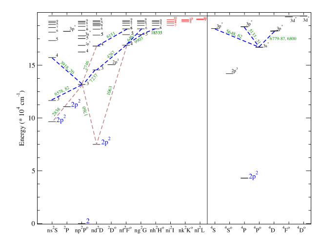
Figure 1: Term diagram for C ii with extended levels. The dashed lines indicate the transitions, from which the investigated spectral lines arise.

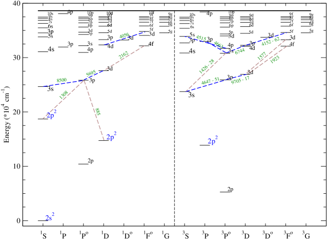
Figure 2: Term diagram for C iii. The dashed lines indicate the transitions, from which the investigated spectral lines arise.

2.2 Method of calculations

To solve the radiative transfer and statistical equilibrium equations, we used the code detail (Butler & Giddings, 1985) based on the accelerated $\Lambda$-iteration method (Rybicki & Hummer, 1991). The detail opacity package was updated by Przybilla et al. (2011) by including bound-free opacities of neutral and ionized species. We then used the code synthV_NLTE (Ryabchikova et al., 2016) to calculate the synthetic NLTE line profiles with the obtained departure coefficients, $b_{\rm{i}}$ = $n_{\rm{NLTE}}$ / $n_{\rm{LTE}}$. Here, $n_{\rm{NLTE}}$ and $n_{\rm{LTE}}$ are the statistical equilibrium and thermal (Saha-Boltzmann) number densities, respectively. Comparison with the observed spectrum and spectral line fitting were performed with the binmag code (Kochukhov, 2010, 2018). For consistency, the calculations were performed with plane-parallel (1D), chemically homogeneous model atmospheres from the Kurucz’s grid (Castelli & Kurucz, 2003) for all stars, including two late O-type stars. We suppose that for O-type stars, the spherical and hydrodynamic NLTE atmospheres would be more physically justified. However, our two O-type stars are unevolved (log $g$ = 3.84 and 4.00) with the simple photospheric physics. They must be unaffected by strong stellar winds unlike the hotter and more luminous supergiants. As for NLTE models, Nieva & Przybilla (2007) demonstrated that, at least, in the range of 20 000 $\leq$ $T_{\rm eff}$ $\leq$ 35 000 K and 3.0 $\leq$ log $g$ $\leq$ 4.5, the hybrid NLTE approach (LTE model atmosphere plus NLTE line formation) is equivalent to full hydrostatic NLTE computations. Although, the temperatures of our O-type stars are higher by $\sim$ 3000 K compared to investigated limit of Nieva & Przybilla (2007), we believe that it will not affect the final results too much.

Table 1 lists lines of C i, C ii, C iii, and C iv used in line formation analyses together with the adopted line data. Oscillator strengths were taken from the NIST database (Kramida et al., 2018). For most lines, Stark collisional data are adopted from the VALD data base.

Table 1: Lines of C i, C ii, C iii, and C iv used in our analysis.

$\lambda$	Transition	$E_{\rm exc}$	log $gf$
Å		eV
C i
9078.28	3s 3Po – 3p 3P	7.48	$-$0.581
9088.51	3s 3Po – 3p 3P	7.48	$-$0.43
9094.83	3s 3Po – 3p 3P	7.49	0.151
9111.80	3s 3Po – 3p 3P	7.49	$-$0.297
9405.73	3s 1Po – 3p 1D	7.49	0.286
9658.43	3s 3Po – 3p 3S	7.49	$-$0.280
C ii
3918.96	3p 2Po – 4s 2S	16.33	$-$0.533
3920.68	3p 2Po – 4s 2S	16.33	$-$0.232
4267.00	3d 2D – 4f 2Fo	18.05	0.563
4267.26	3d 2D – 4f 2Fo	18.05	0.716
4267.26	3d 2D – 4f 2Fo	18.05	$-$0.584
5132.95	2p3s 4Po – 2p3p 4P	20.70	$-$0.211
5133.28	2p3s 4Po – 2p3p 4P	20.70	$-$0.178
5137.25	2p3s 4Po – 2p3p 4P	20.70	$-$0.911
5139.17	2p3s 4Po – 2p3p 4P	20.70	$-$0.707
5143.49	2p3s 4Po – 2p3p 4P	20.70	$-$0.212
5145.16	2p3s 4Po – 2p3p 4P	20.71	0.189
5151.09	2p3s 4Po – 2p3p 4P	20.71	$-$0.179
5648.07	3s 4Po – 3p 4S	20.70	$-$0.424
5662.47	3s 4Po – 3p 4S	20.70	$-$0.249
6151.26	4d 2D – 6f 2Fo	20.84	$-$0.164
6151.53	4d 2D – 6f 2Fo	20.84	$-$1.310
6151.53	4d 2D – 6f 2Fo	20.84	$-$0.009
6461.94	4f 2Fo – 6g 2G	20.95	0.161
6461.94	4f 2Fo – 6g 2G	20.95	0.048
6461.94	4f 2Fo – 6g 2G	20.95	$-$1.383
6578.05	3s 2S – 3p 2Po	14.45	$-$0.021
6582.88	3s 2S – 3p 2Po	14.45	$-$0.323
6779.94	3s 4Po – 3p 4D	20.70	0.025
6780.59	3s 4Po – 3p 4D	20.70	$-$0.377
6783.90	3s 4Po – 3p 4D	20.70	0.304
6800.68	3s 4Po – 3p 4D	20.70	$-$0.343
9903.46	4f 2Fo – 5g 2G	20.95	$-$0.523
9903.46	4f 2Fo – 5g 2G	20.95	0.908
9903.46	4f 2Fo – 5g 2G	20.95	1.021
18 535.94	5g 2G – 6h 2Ho	22.20	1.217
18 535.94	5g 2G – 6h 2Ho	22.20	1.129
18 535.94	5g 2G – 6h 2Ho	22.20	$-$0.515
C iii
4056.06	4d 1D – 5f 1Fo	40.19	0.267
4152.51	3p 3D – 5f 3Fo	40.05	$-$0.112
4162.86	3p 3D – 5f 3Fo	40.06	0.218
4516.00	4p 3Po – 5s3S	39.40	$-$0.058
4647.42	3s 3S – 3p 3Po	29.53	0.070
4650.25	3s 3S – 3p 3Po	29.53	$-$0.151
4651.47	3s 3S – 3p 3Po	29.53	$-$0.629
4652.05	3s 3Po – 3p 3P	38.21	$-$0.432
4663.64	3s 3Po – 3p 3P	38.21	$-$0.530
4665.86	3s 3Po – 3p 3P	38.22	0.044
5695.92	3p 1Po – 3d 1D	32.10	0.017
6731.04	3s 3Po – 3p 3D	38.22	$-$0.293
6744.39	3s 3Po – 3p 3D	38.22	$-$0.022
7037.25	3s 1Po – 4d 1D	38.44	0.443
8500.32	3s 1S – 3p 1Po	30.64	$-$0.484
9705.41	3p 3Po – 3d 3D	32.20	$-$0.378
9706.44	3p 3Po – 3d 3D	32.20	$-$0.855
9715.09	3p 3Po – 3d 3D	32.20	$-$0.107
9717.75	3p 3Po – 3d 3D	32.20	$-$0.855
C iv
5801.31	3s 2S – 3p 2Po	37.55	$-$0.194
5811.97	3s 2S – 3p 2Po	37.55	$-$0.495

2.3 Departures from LTE for C ii – C iii in B-type star

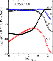
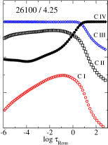
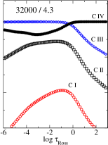
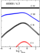
Figure 3: Ionization fractions of C i, C ii, C iii, and C iv in the model atmospheres of different effective temperatures.

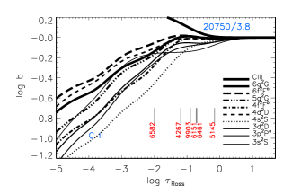
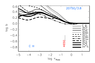
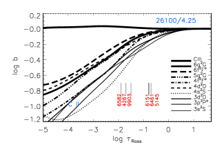
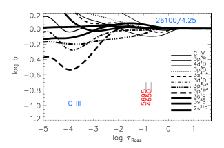
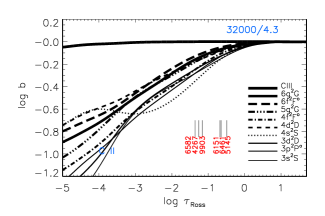
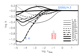
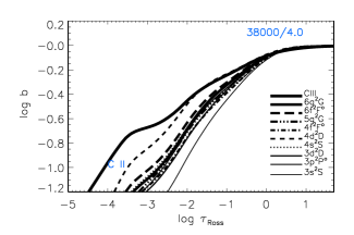
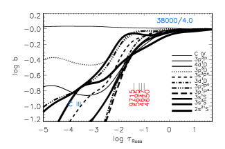
Figure 4: Departure coefficients for the C ii and C iii levels as a function of $\log\tau_{Ross}$ in the model atmospheres with $T_{\rm eff}$/log $g$ = 20750 / 3.8; 26100/ 4.25; 32000 / 4.3; and 38000 / 4.0. The vertical lines indicate the formation depths of cores of individual lines.

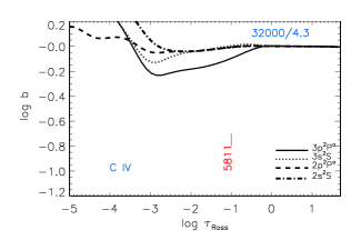
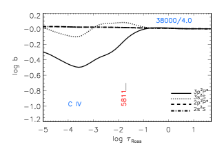
Figure 5: Departure coefficients for the C iv levels as a function of $\log\tau_{Ross}$ in the model atmospheres with $T_{\rm eff}$/log $g$ = 32000 / 4.3; and 38000 / 4.0.

Figure 3 displays the ionization fraction of different carbon ions C i, C ii, C iii, and C iv in stellar atmospheres of different effective temperatures. In the atmospheres with $T_{\rm eff}$ $\lesssim$ 32 000 K, C iii is the dominant ionization stage in the line-formation region, while C iv becomes the major species in the hotter atmospheres.

Figures 4 and 5 show the departure coefficients for the selected levels in the model atmospheres with $T_{\rm eff}$/log $g$ = 20 750 / 3.8, 26 100 / 4.25, 32 000 / 4.3, and 38 000 / 4.0. The departure coefficients are equal to unity deep in the atmosphere, where the gas density is large and collisional processes dominate, enforcing the LTE.

In the models 20 750 / 3.8, 26 100 / 4.25, and 32 000 / 4.3, the NLTE leads to depleted populations of the C ii levels because of UV overionization, while in the last two models the C iii ground state is close to the TE population, since doubly ionized carbon dominates the element abundance outwards log $\tau_{Ross}=0$.

In the model 20 750 / 3.8, outward of log $\tau_{Ross}=-0.2$, the C iii ground state is overpopulated via photoionization processes C ii+ h$\nu$ $\rightarrow$ C iii+e^-, and the overpopulation is extended to the remaining C iii levels due to their coupling to the ground state. In hotter atmospheres 26 100 / 4.25 and 32 000 / 4.3, spontaneous transitions dominate, resulting in a depopulation of the C iii levels, while the C iii ground state keeps its LTE populations.

In the model 38 000 / 4.0, outward of log $\tau_{Ross}=0.3$, NLTE leads to depleted populations of the C ii and C iii levels because of UV overionization, while the C iv ground state almost keeps its LTE populations.

Analysis of the departure coefficients of the lower (b_l) and upper (b_u) levels at the line-formation depths allows to understand NLTE effects for a given spectral line. If b${}_{l}>$ 1 and (or) the line source function is smaller than the Planck function, that is, b${}_{l}>$ b_u, a NLTE strengthening of lines occurs. The carbon lines of four ionization stages are listed in Table 1.

C ii 4267 Å This line, arising from 3d ²D – 4f ²F^o, is strong. In the 20 750 / 3.8 model, its core forms at atmospheric depths ($\log\tau_{Ross}=-1.2$) dominated by overionization of C ii, resulting in the weakened line and positive abundance correction, $\Delta_{\rm NLTE}$ = log$\epsilon_{\rm NLTE}$ - log$\epsilon_{\rm LTE}$, which equals to +0.25 dex. In the model 26 100 / 4.25, the line shifts to the outer layers, where the deviations from LTE are strong and abundance correction amounts to +0.77 dex. While in the model 32 000 / 4.3, the line shifts to the inner layers and $\Delta_{\rm NLTE}$ = +0.33 dex.

C ii 6151, 6461 Å These lines, arising from 4d ²D – 6f ²F^o, 4f ²F^o – 6g ²G, are weak and their cores form at atmospheric depths around $\log\tau_{Ross}=-0.75$ in the models 20 750 / 3.8, 26 100 / 4.25, and 32 000 / 4.3, where b${}_{l}<$ b_u and b${}_{l}<$1, that leads to weakening of these lines. The abundance corrections for C ii 6151 Å are $\Delta_{\rm NLTE}$ = +0.28, +1.19 dex in the 20 750 / 3.8, 26 100 / 4.25 models, respectively, while it appears as weak emission line in 32 000 / 4.3. For C ii 6461 Å, $\Delta_{\rm NLTE}$ = +0.38 dex in the 20 750 / 3.8, while this line appears as emission in the hotter models.

C ii 6582 Å This line, together with 6578, arising from 3s ²S – 3p ²P^o, is strong and in the model 20 750 / 3.8 its core forms around $\log\tau_{Ross}=-2.0$, where the departure coefficient of the upper level 3p ²P^o drops rapidly. This results in dropping the line source function below the Planck function and enhancing absorption in the line core. In contrast, in the line wings, absorption is weaker compared with the LTE case due to overall overionization. As a result the abundance correction is slightly negative $-$0.16 dex. In the 26 100 / 4.25 and 32 000 / 4.3 models, the overionization of C ii leads to weakening of these lines and results in positive abundance corrections, +0.45 and +0.22 dex, respectively. Moreover, these lines are lying in the wing of the H$\alpha$ line at 6563Å. This makes the formation of these lines very sensitive to modeling of the hydrogen line formation.

C ii 9903 Å This line, arising from 4f ²F^o – 5g ²G, is strong. In the line formation region, $\log\tau_{Ross}\sim-1.25$, b${}_{l}<$ b_u and b${}_{l}<$1, that leads to weakening of the line. It appears as an emission line in the presented models with $T_{\rm eff}$ from 17 500 to 33 400 K, and disappears when $T_{\rm eff}$ is higher than 33 400 K.

C iii 4650 Å This line, as with 4647 Å and 4651 Å lines, arising from 3s ³S – 3p ³P^o, is strong and in the models 20 750 / 3.8, 26 100 / 4.25, and 32 000 / 4.3, b${}_{l}>$ b_u in the line formation region and the line source function drops below the Planck function resulting in strengthened lines and negative NLTE abundance corrections of $\Delta_{\rm NLTE}$ = $-$0.23 dex, $-$0.33 dex, $-$0.61 dex respectively. In the model 38 000 / 4.0 b${}_{l}<$ b_u in the line formation region, which leads to weakening of the line and $\Delta_{\rm NLTE}$ = $+$0.64 dex.

C iii 5695 Å The line, arising from 3p ¹P^o – 3d ¹D, is strong. Its core forms at atmospheric depths around $\log\tau_{Ross}=-1.0$. The line has slightly negative abundance correction, $-$0.12, in the model 26 100 / 4.25 and slightly positive one, +0.06 dex, in 32 000 / 4.3. In the model 38 000 / 4.0, the line formation region moves to inner layers, where b${}_{l}<$ b_u, and b${}_{l}<$1, and the line appears in emission.

C iv 5811 Å This line and 5801 Å arising from 3s ²S – 3p ²P^o, appear to be stronger in the hotter atmospheres. In the line formation region b${}_{l}>$ b_u that results in strengthened line and negative NLTE abundance correction of $\Delta_{\rm NLTE}$ = $-$0.37 dex in the model 32 000 / 4.3. In a hotter model, 38 000 / 4.0, line formation region moves to outer layers (Fig. 5), where the departures from LTE are stronger. So, in the model 38 000 / 4.0 the NLTE abundance correction is $-$1.29 dex.

2.4 C i emission lines

The mechanisms driving the C i emission were described in details in Alexeeva et al. (2016). Our NLTE calculations predicted that C i emission lines to appear at effective temperature from 9250 to 10 500 K depending on log $g$. They are near IR C i lines at 8335 Å (3s ¹P^o – 3p ¹S) and 9405 Å (3s ¹P^o – 3p ¹D) singlet lines and at higher temperature, $T_{\rm eff}$$>$ 15 000 K (log $g$ = 4), in the 9061–9111 Å (3s ³P^o – 3p ³P), and 9603–9658 Å (3s ³P^o – 3p ³S) triplet lines. Having appeared at specific $T_{\rm eff}$/log $g$, the emission is strengthened towards higher temperature, reaches its maximum and disappears at about $T_{\rm eff}$$=$ 22 000 K (in the case of log $g$ = 3).

2.5 C ii emission lines

Our NLTE calculations in the grid of model atmospheres with 18 000 K $\leq$ $T_{\rm eff}$ $\leq$ 35 000 K and log $g$ = 4 predict that C ii lines at 6151 Å (4d ²D – 6f ²F^o), 6461 Å (4f ²F^o – 6g ²G), 9903 Å (4f ²F^o – 5g ²G), and 18 535 Å (5g ²G – 6h ²H^o) may appear as emission lines depending on the atmospheric parameters (Fig. 6). The NET rates, that were calculated as NET = $n_{\rm{l}}$($R_{\rm{lu}}$ + $C_{\rm{lu}}$)$-$$n_{\rm{u}}$ ($R_{\rm{ul}}$ + $C_{\rm{ul}}$), allow to know what processes in C ii do drive the emission in the lines. Here, $R_{\rm{lu}}$ and $C_{\rm{lu}}$ are radiative and collisional rates, respectively, for the transition from low to upper level, and $R_{\rm{ul}}$ and $C_{\rm{ul}}$ for the inverse transition. The upper levels of the investigated transitions, 6f ²F^o, 5g ²G, 6g ²G, 6h ²H^o, are mainly populated by recombination from C iii and cascade transitions from Rydberg states, while the low-excitation levels (4d ²D and 4f ²F^o) have depleted populations due to photon losses in the lines of C ii arising from the transitions 3p ²P^o – 4d ²D (2746 Å) and 3d ²D – 4f ²F^o (4267 Å). Extra depopulation of the level 4f ²F^o is caused by overionization. These mechanisms result in a depopulation of the lower levels to a greater extent than the upper levels and are responsible for the emission phenomenon. Test calculations with the model atom, where the Rygberg states ($l>$6) were not included, demonstrate the decrease of the relative flux at the line center of C ii 9903 Å from 1.30 to 1.06 in the model atmosphere 26 100 / 4.25. It demonstrates a crucial role of these Rygberg states in emission phenomenon at C ii 9903 Å.

2.6 C iii emission lines

Our NLTE calculations predict that the emission lines of C iii at 5695 Å (3p ¹P^o – 3d ¹D) and those of 6727–6762 Å (3s ³P^o – 3p ³D) and 9705–9717 Å (3p ³P^o – 3d ³D) to appear at effective temperature $T_{\rm eff}$$>$ 35 000 K (log $g$ = 4). The emission line of C iii 7037 Å (3s ¹P^o – 4d ¹D) appears at effective temperature $T_{\rm eff}$$>$ 37 000 K (log $g$ = 4) (Fig. 6). The analysis of NET values and test calculations show that the photoionization-recombination mechanisms play a crucial role in emission line formation. The lower levels of investigated transitions, 3p ¹P^o, 3s ³P^o, and 3p ³P^o, are depopulated due to ionization, while the upper levels, 3d ¹D, 3p ³D, and 3d ³D are populated due to recombination from C iv reservoir. Extra depopulation of the levels 3p ¹P^o and 3s ³P^o is caused by photon losses in UV transitions 2p^{2 1}D – 3p ¹P^o (885 Å), 2p^{2 1}S – 3p ¹P^o (1308 Å), 3s ³S – 3s ³P^o (1426 – 1428 Å). The upper level 3d ³D is effectively populated due to transitions 3d ³D – 3d ³F^o (1577 Å) and 3d ³D – 4f ³F^o (1923 Å).

On the base of the structure of terms (Fig. 2), the C iii 9705–9717 Å triplet lines are similar to the 5695 Å singlet line. The intensity of emission line at 9705–9717 Å is higher than 5695 Å. There are two reasons for the difference: its position in the near-IR region, where the continuum flux is lower, and the line formation region of 9705–9717 Å is located closer to outer layers (Fig. 4), where the deviations from LTE are stronger.

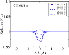
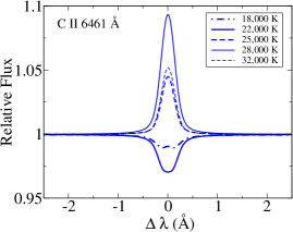
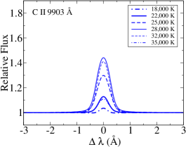
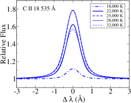
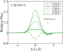
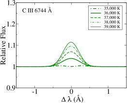
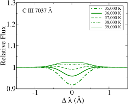
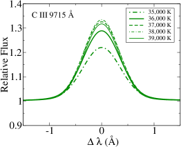
Figure 6: Evolutions of the C ii 6151, 6461, 9903, and 18 535 Å, and C iii 5695, 6744, 7037 and 9715 Å, line profiles with the effective temperature. In every cases, we assume A(C)=8.43, $v$ sin $i$ = 10 km s^-1, and $\xi_{t}$ = 2 km s^-1. The theoretical spectra are convolved with an instrumental profile of R = 50 000.

3 Carbon lines in the selected stars

3.1 Stellar sample, Observations, and stellar parameters

We analyse high resolution spectral data of 22 stars listed in Table 2. The sample contains 20 B-type stars (ranging in spectral types from B3 to B0) and two O-type stars. All of these stars show relatively sharp spectral lines (slowly rotating). Atmospheric parameters of 20 B-type stars are taken from Nieva & Przybilla (2012) or from Nieva & Simón-Díaz (2011). Those of 15 Mon (HD 47839) and HD 42088 are taken from Markova et al. (2004) and from Martins et al. (2015c), respectively.

Spectral data from the visible to near IR spectral ranges were obtained with the Echelle Spectro Polarimetric Device for the Observation of Stars (ESPaDOnS) (Donati et al., 2006) attached to the 3.6 m telescope of the Canada-France-Hawaii Telescope (CFHT) observatory located on the summit of Mauna Kea, Hawaii. Observations with this spectrograph cover the region from 3690 to 10480 Å, and we use data from 3855 to 9980 Å in the present study. The resolving power is $\it R$ = 65 000. Calibrated intensity spectral data were extracted from the ESPaDOnS archive through Canadian Astronomical Data Centre (CADC).

After averaging downloaded individual spectral data of each star, we converted the wavelength scale of spectral data of each star into the laboratory scale using measured wavelengths of five He i lines (4471.48, 4713.15, 4921.93, 5015.68, and 5875.62 Å). In the case of O-type stars, we add measured wavelengths of two He ii lines (4685.68 Å and 5411.52 Å). Errors in the wavelength measurements are around $\pm$ 3 km s^-1 or smaller. Re-fittings of the continuum level of each spectral order were carried out using polynomial functions. The signal-to-noise ratios (SN) measured at the continuum near 5550 Å range from 380 to 1800. Five stars among the sample show very high qualities (SN ratio higher than 1000).

Table 2: Atmospheric parameters of the selected stars, SN ratio, and sources of the data.

Number	Star	Name	Sp. T.	$T_{\rm eff}$	log $g$	$\xi_{t}$	$V_{mac}$	$v$ sin $i$	SN	Ref.
				K	CGS	km s-1	km s-1	km s-1
1	HD 209008	18 Peg	B3 III	15 800	3.75	4	10	15	710	1
2	HD 160762	$\iota$ Her	B3 IV	17 500	3.80	1		6	1820	1
3	HD 35912	HR 1820	B2-3 V	19 000	4.00	2	8	15	650	2
4	HD 36629	HIP 26000	B2 V	20 300	4.15	2	5	10	630	2
5	HD 35708	$o$ Tau	B2.5 IV	20 700	4.15	2	17	25	820	1
6	HD 3360	$\zeta$ Cas	B2 IV	20 750	3.80	2	12	20	1570	1
7	HD 122980	$\chi$ Cen	B2 V	20 800	4.22	3		18	520	1
8	HD 16582	$\delta$ Cet	B2 IV	21 250	3.80	2	10	15	1050	1
9	HD 29248	$\nu$ Eri	B2 II	22 000	3.85	6	15	26	550	1
10	HD 886	$\gamma$ Peg	B2 IV	22 000	3.95	2	8	9	1110	1
11	HD 74575	$\alpha$ Pix	B1.5 III	22 900	3.60	5	20	11	800	1
12	HD 35299	HR 1781	B2 III	23 500	4.20	0		8	380	1
13	HD 36959	HR 1886	B1 V Ic	26 100	4.25	0	5	12	860	2
14	HD 61068	HR 2928	B2 II	26 300	4.15	3	20	14	560	1
15	HD 36591	HR 1861	B2 III	27 000	4.12	3		12	720	1
16	HD 37042	$\theta^{2}$ Ori B	B0.5 V	29 300	4.30	2	10	30	690	2
17	HD 36822	$\phi^{1}$ Ori	B0.5 III	30 000	4.05	8	18	28	570	1
18	HD 34816	$\lambda$ Lep	B0.5 V	30 400	4.30	4	20	30	550	1
19	HD 149438	$\tau$ Sco	B0.2 V	32 000	4.30	5	4	4	1730	1
20	HD 36512	$\upsilon$ Ori	B0 V	33 400	4.30	4	10	20	700	1
21	HD 47839	15 Mon	O7 V	37 500	3.84	12	65∗	62	560	3
22	HD 42088		O6 V	38 000	4.00	12∗∗	37	41	820	4

Note. — Note. References: 1 Nieva & Przybilla (2012); 2 Nieva & Simón-Díaz (2011); 3 Markova et al. (2004); 4 Martins et al. (2015c). ^∗ Simón-Díaz et al. (2017) ; ^∗∗ Holgado et al. (2018). Spectral types are extracted from the SIMBAD database. (10) Measured SN ratio near 5550 Å.

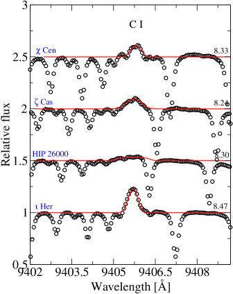
Figure 7: Best NLTE fits (solid curves) of C i 9405 Å in $\iota$ Her, HIP 26000, $\zeta$ Cas, and $\chi$ Cen. The observed spectra are shown by open circles.

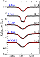
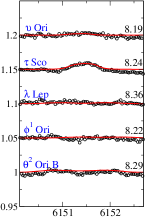
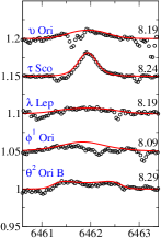
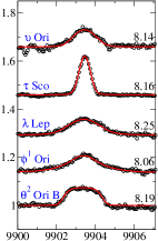
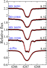
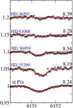
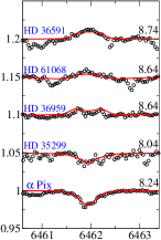
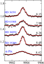
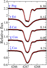
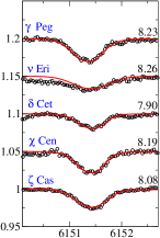
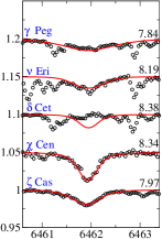
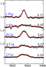
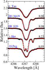
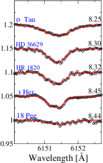
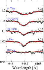
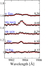
Figure 8: Best NLTE fits (solid curves) of C ii 4267, 6151, 6461, and 9903 Å in the program stars (from left to right). The observed spectra are shown by open circles.

3.2 Determination of carbon abundances in B-stars

In this section, we derive the carbon abundances of the selected B-stars from emission C i, emission and absorption C ii  and absorption C iii lines using the atomic data from Table 1. In Table 3, we show the NLTE and LTE abundances derived from absorption and emission lines by the spectrum fitting method. Emission lines are marked by $e$ in the corresponding LTE columns. The averaged NLTE abundances obtained from emission and absorption lines of four ionization stages are shown in Table 5.

Emission lines of C i were detected in the observed spectra of the five stars: $\iota$ Her, HR 1820, HIP 26000, $\zeta$ Cas, and $\chi$ Cen. In the spectra of 18 Peg and $o$ Tau, the C i lines were not used, because they are blended with telluric lines located in near-IR spectral region. All the C i lines almost disappear in the spectra of stars with $T_{\rm eff}$ higher than 22 000 K, because carbon become predominantly singly- or doubly ionized (Fig. 3). For each star, our NLTE calculations reproduce well the observed C i emission lines, using our model atom and adopted atmospheric parameters. The best NLTE fits of the C i 9405 Å emission lines in $\iota$ Her, HIP 26000, $\zeta$ Cas, and $\chi$ Cen are presented in Fig. 7.

The C ii emission line at 9903 Å was detected in the observed spectra of all B-type stars in our sample. The hotter stars, HR 1886, HR 2928, HR 1861, $\theta^{2}$ Ori B, $\phi^{1}$ Ori, $\lambda$ Lep, $\tau$ Sco, and $\upsilon$ Ori, also have the emission lines at 6461 Å in their spectra, and the five B-type stars show the emission lines at 6151 Å, too. The best fits of C ii 4267, 6151, 6461, and 9903 Å, are presented in Figure 8. For each star, our NLTE calculations reproduce satisfactorily the observed C ii 6151, 6461 Å absorption and emission lines. In four stars, $\iota$ Her, $\delta$ Cet, $\gamma$ Peg, and HR 1861, we excluded the abundances obtained from C ii 6151 and 6461 Å lines in the mean value, because these two lines give apparently discrepant abundances among other lines. It should be noticed that these two lines are sensitive to the choice of threshold photoionization cross sections, that were corrected one order of magnitude higher for the upper levels, 6f ²F^o and 6g ²G, of investigated transitions.

The C iii 8500 Å line should be considered with caution, because it is lying almost in the core of the broad Paschen P16 line at 8502.5 Å, which also was included in spectral synthesis. We analysed this line in seven stars and the derived abundances were found to be consistent with other C iii lines.

For each star, NLTE provides smaller line-to-line scatter that is illustrated in Fig. 9 (left panel). The ionization equilibrium C i/C ii/C iii was achieved for the four stars, and C ii/C iii for eleven stars of our sample. For two stars, $\tau$ Sco and $\upsilon$ Ori, we obtained abundances from three ionization stages, C ii/C iii/C iv. C ii/C iii ionization equilibrium is achieved in $\tau$ Sco, however the abundance from C iv lines is lower, although still consistent within 2$\sigma$. C ii/C iv ionization equilibrium is achieved in $\upsilon$ Ori, however the abundance from C iii lines gives a higher abundance than that from the C ii and C iv lines, by 0.23 and 0.22 dex, respectively. In both stars, the abundances from C iii lines are higher compared to C ii and C iv. For $\phi^{1}$ Ori, $\lambda$ Lep, $\tau$ Sco the NLTE abundances derived from the C ii and C iii lines agree within the error bars, while in LTE, the abundance differences can reach up to 0.72 dex.

We obtained an averaged abundance of carbon log $\epsilon_{\rm C}$=8.36$\pm$0.08 from twenty B-type stars from all lines listed in Table 3. The resulting value is lower by $\sim$0.07 dex compared to the solar carbon NLTE abundance, log $\epsilon_{\rm C}$=8.43, which are obtained with this model atom from C i atomic lines in Alexeeva & Mashonkina (2015). Our result is in line with the present-day Cosmic Abundance Standard (Nieva & Przybilla, 2012), where log $\epsilon_{\rm C}$=8.33$\pm$0.04 is presented.

3.3 Determination of carbon abundances in O-stars

Here, we derive the carbon abundances of two O-type stars from emission and absorption C iii and absorption C iv lines by spectrum fitting. In Table 4, we present the abundances derived from absorption and emission lines in two O-type stars. Best NLTE fits of C iii 5695, 6744, 8500, and 9701–17 Å and C iv 5801, 5811 Å in HD 42088 and 15 Mon are presented on Figure 10. Everywhere NLTE provides smaller line-to-line scatter that is illustrated by Fig. 9 (right panel). The abundances derived from emission and absorption C iii are slightly lower (by $\sim$0.14 dex) compared to C iv, although still consistent within the error bars. In both stars, NLTE provides consistent values within 0.14 dex abundances from the two ionization stages, C iii and C iv, while the LTE abundance difference can be up to 1.34 dex in the absolute value. It should be noticed that emission lines of C iii 9705–17 Å tend to be stronger in our modeling, that leads to lower abundances from this line in both stars. After excluding C iii 9705–17 Å lines, we obtained log $\epsilon_{\rm C}$=8.31$\pm$0.11 in HD 42088 and log $\epsilon_{\rm C}$=8.27$\pm$0.08 in 15 Mon from the lines of both ionization stages.

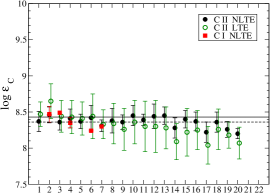
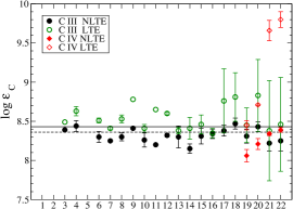
Figure 9: Carbon LTE and NLTE abundances of program stars derived from lines of C i, C ii (left panel) and C iii, C iv (right panel). The horizontal axis corresponds to the serial number of star, according to Table 2. The error bars correspond to the dispersion in the single-line measurements about the mean. In each panel, the dashed line represents the NLTE abundance averaged over all C i, C ii, C iii, and C iv lines, log $\epsilon_{\rm C}$=8.36. The solid line represents the solar value, log $\epsilon_{\rm C}$=8.43.

Table 3: NLTE and LTE Carbon abundances in 20 B-type stars.

$\lambda$ (Å )	NLTE	LTE	NLTE	LTE	NLTE	LTE	NLTE	LTE	NLTE	LTE	NLTE	LTE	NLTE	LTE	NLTE	LTE	NLTE	LTE	NLTE	LTE
	18 Peg		$\iota$ Her		HR 1820		HIP 26000		$o$ Tau		$\zeta$ Cas		$\chi$ Cen		$\delta$ Cet		$\nu$ Eri		$\gamma$ Peg
Cı
9078	$\cdots$	$\cdots$	8.62	$e$	$\cdots$	$\cdots$	$\cdots$	$\cdots$	$\cdots$	$\cdots$	$\cdots$	$\cdots$	$\cdots$	$\cdots$	$\cdots$	$\cdots$	$\cdots$	$\cdots$	$\cdots$	$\cdots$
9088	$\cdots$	$\cdots$	8.51	$e$	$\cdots$	$\cdots$	8.40	$e$	$\cdots$	$\cdots$	$\cdots$	$\cdots$	$\cdots$	$\cdots$	$\cdots$	$\cdots$	$\cdots$	$\cdots$	$\cdots$	$\cdots$
9094	$\cdots$	$\cdots$	8.39	$e$	8.49	$e$	$\cdots$	$\cdots$	$\cdots$	$\cdots$	$\cdots$	$\cdots$	8.29	$e$	$\cdots$	$\cdots$	$\cdots$	$\cdots$	$\cdots$	$\cdots$
9111	$\cdots$	$\cdots$	8.47	$e$	$\cdots$	$\cdots$	$\cdots$	$\cdots$	$\cdots$	$\cdots$	8.23	$e$	8.29	$e$	$\cdots$	$\cdots$	$\cdots$	$\cdots$	$\cdots$	$\cdots$
9405	$\cdots$	$\cdots$	8.47	$e$	$\cdots$	$\cdots$	8.30	$e$	$\cdots$	$\cdots$	8.24	$e$	8.33	$e$	$\cdots$	$\cdots$	$\cdots$	$\cdots$	$\cdots$	$\cdots$
9658	$\cdots$	$\cdots$	8.29	$e$	$\cdots$	$\cdots$	$\cdots$	$\cdots$	$\cdots$	$\cdots$	$\cdots$	$\cdots$	$\cdots$	$\cdots$	$\cdots$	$\cdots$	$\cdots$	$\cdots$	$\cdots$	$\cdots$
Mean	$\cdots$	$\cdots$	8.47	$\cdots$	8.49	$\cdots$	8.35	$\cdots$	$\cdots$	$\cdots$	8.24	$\cdots$	8.30	$\cdots$	$\cdots$	$\cdots$	$\cdots$	$\cdots$	$\cdots$	$\cdots$
$\sigma$	$\cdots$	$\cdots$	0.11	$\cdots$	$\cdots$	$\cdots$	0.07	$\cdots$	$\cdots$	$\cdots$	0.01	$\cdots$	0.02	$\cdots$	$\cdots$	$\cdots$	$\cdots$	$\cdots$	$\cdots$	$\cdots$
C ii
3918	8.30	8.35	8.33	8.50	8.24	8.24	8.24	8.24	$\cdots$	$\cdots$	8.30	8.32	8.21	8.16	8.11	8.10	8.43	8.09	8.26	8.15
3920	8.30	8.24	8.28	8.51	8.23	8.30	8.24	8.28	$\cdots$	$\cdots$	8.25	8.34	8.20	8.23	8.09	8.09	$\cdots$	$\cdots$	8.26	8.21
4267	8.05	8.24	8.23	8.42	8.08	8.12	8.08	8.02	8.14	8.03	8.21	7.96	8.09	7.90	8.14	7.72	8.14	7.63	8.30	7.83
5132	8.43	8.46	8.52	8.54	8.42	8.41	8.43	8.44	8.34	8.34	8.41	8.39	8.32	8.30	8.30	8.24	8.42	8.35	8.46	8.38
5137	$\cdots$	$\cdots$	8.54	8.53	8.44	8.46	8.40	8.41	8.35	8.31	8.48	8.44	8.41	8.41	8.31	8.25	8.44	8.19	8.47	8.39
5139	$\cdots$	$\cdots$	8.47	8.47	8.44	8.40	8.34	8.35	8.35	8.35	8.43	8.35	8.28	8.23	8.29	8.23	8.42	8.22	8.46	8.37
5143	8.48	8.58	8.53	8.57	8.44	8.45	8.43	8.44	8.36	8.39	8.44	8.42	8.34	8.33	8.37	8.31	8.42	8.36	8.47	8.45
5145	8.46	8.49	8.55	8.63	8.43	8.49	8.49	8.51	8.36	8.43	8.49	8.45	8.36	8.37	8.39	8.33	8.44	8.36	8.47	8.47
5151	8.48	8.50	8.53	8.56	8.41	8.41	8.44	8.46	8.35	8.36	8.44	8.43	8.35	8.36	8.35	8.29	8.45	8.38	8.46	8.45
5648	$\cdots$	$\cdots$	8.46	8.59	8.46	8.55	8.40	8.49	8.39	8.48	8.37	8.47	8.38	8.44	8.26	8.36	8.31	8.45	8.35	8.44
5662	$\cdots$	$\cdots$	8.43	8.52	8.37	8.45	8.32	8.41	8.26	8.34	8.24	8.35	8.21	8.29	8.15	8.27	8.25	8.42	8.30	8.40
6151	8.44	8.51	8.45	8.28	8.32	8.09	8.30	8.03	8.25	8.04	8.08	7.80	8.19	7.98	7.90∗	7.58∗	8.26	7.80	8.23	7.77
6461	8.44	8.14	8.74∗	8.17∗	8.32	7.86	8.30	7.85	8.21	7.84	7.97	7.59	8.34	7.92	$\cdots$	$\cdots$	8.19	7.50	7.84∗	7.44∗
6578	8.23	8.66	8.36	9.13	8.18	8.94	8.31	8.79	8.39	8.81	8.59	8.93	8.26	8.70	8.62	8.82	$\cdots$	$\cdots$	8.67	8.65
6582	8.26	8.66	8.42	9.12	8.22	8.79	8.37	8.73	8.45	8.72	8.67	8.83	8.33	8.59	8.72	8.65	$\cdots$	$\cdots$	8.77	8.62
6779	$\cdots$	$\cdots$	$\cdots$	$\cdots$	8.40	8.35	8.46	8.42	8.41	8.36	8.45	8.39	8.36	8.29	8.33	8.23	8.28	8.30	8.47	8.36
6780	$\cdots$	$\cdots$	$\cdots$	$\cdots$	8.40	8.35	8.46	8.44	8.41	8.36	8.45	8.39	8.36	8.29	8.33	8.23	8.28	8.30	8.47	8.36
6783	$\cdots$	$\cdots$	8.61	8.63	8.53	8.47	8.59	8.52	8.49	8.44	8.62	8.51	8.40	8.35	8.47	8.35	8.42	8.40	8.59	8.46
6800	$\cdots$	$\cdots$	$\cdots$	$\cdots$	8.40	8.36	8.46	8.41	8.41	8.36	8.47	8.39	8.35	8.31	8.32	8.23	8.36	8.38	8.42	8.32
9903	$\cdots$	$\cdots$	8.50	$e$	8.29	$e$	8.68	$e$	8.54	$e$	8.50	$e$	8.33	$e$	8.61	$e$	8.44	$e$	8.37	$e$
Mean	8.37	8.47	8.46	8.65	8.36	8.44	8.41	8.43	8.37	8.41	8.42	8.44	8.31	8.33	8.38	8.34	8.36	8.26	8.45	8.36
$\sigma$	0.14	0.17	0.11	0.24	0.11	0.22	0.13	0.23	0.10	0.23	0.17	0.31	0.08	0.20	0.17	0.28	0.10	0.29	0.14	0.30
C iii
4647	$\cdots$	$\cdots$	$\cdots$	$\cdots$	8.39	8.49	8.39	8.58	$\cdots$	$\cdots$	8.23	8.47	8.24	8.39	8.24	8.47	8.41	8.78	$\cdots$	$\cdots$
4650	$\cdots$	$\cdots$	$\cdots$	$\cdots$	$\cdots$	$\cdots$	8.49	8.67	$\cdots$	$\cdots$	8.30	8.53	8.26	8.42	8.31	8.55	$\cdots$	$\cdots$	8.17	8.43
4651	$\cdots$	$\cdots$	$\cdots$	$\cdots$	$\cdots$	$\cdots$	$\cdots$	$\cdots$	$\cdots$	$\cdots$	8.36	8.53	$\cdots$	$\cdots$	8.34	8.57	$\cdots$	$\cdots$	8.25	8.44
5696	$\cdots$	$\cdots$	$\cdots$	$\cdots$	$\cdots$	$\cdots$	$\cdots$	$\cdots$	$\cdots$	$\cdots$	$\cdots$	$\cdots$	$\cdots$	$\cdots$	$\cdots$	$\cdots$	$\cdots$	$\cdots$	8.34	8.35
Mean	$\cdots$	$\cdots$	$\cdots$	$\cdots$	8.39	8.49	8.44	8.63	$\cdots$	$\cdots$	8.30	8.51	8.25	8.41	8.30	8.53	8.41	8.78	8.26	8.41
$\sigma$	$\cdots$	$\cdots$	$\cdots$	$\cdots$	$\cdots$	$\cdots$	0.07	0.06	$\cdots$	$\cdots$	0.07	0.03	0.01	0.02	0.05	0.05	$\cdots$	$\cdots$	0.09	0.05
	$\alpha$ Pix		HR 1781		HR 1886		HR 2928		HR 1861		$\theta^{2}$ Ori B		$\phi^{1}$ Ori		$\lambda$ Lep		$\tau$ Sco		$\upsilon$ Ori
C ii
3918	8.36	8.26	8.19	8.09	8.29	8.13	$\cdots$	$\cdots$	$\cdots$	$\cdots$	$\cdots$	$\cdots$	8.26	8.18	$\cdots$	$\cdots$	8.25	8.25	8.31	8.26
3920	$\cdots$	$\cdots$	8.19	8.13	8.20	8.06	8.15	7.93	$\cdots$	$\cdots$	$\cdots$	$\cdots$	$\cdots$	$\cdots$	$\cdots$	$\cdots$	$\cdots$	$\cdots$	$\cdots$	$\cdots$
4267	8.41	7.70	8.33	7.72	8.41	7.64	8.24	7.54	8.27	7.55	8.22	7.58	8.19	7.75	8.22	7.71	8.15	7.82	8.14	8.03
5132	8.42	8.33	8.49	8.38	8.54	8.35	8.33	8.14	8.51	8.32	8.51	8.30	8.34	8.17	8.48	8.31	8.39	8.24	$\cdots$	$\cdots$
5137	8.43	8.42	8.52	8.40	8.54	8.34	8.31	8.14	8.47	8.29	8.47	8.27	$\cdots$	$\cdots$	$\cdots$	$\cdots$	$\cdots$	$\cdots$	$\cdots$	$\cdots$
5139	8.42	8.34	8.45	8.34	8.55	8.34	8.27	8.09	8.45	8.27	8.53	8.33	$\cdots$	$\cdots$	$\cdots$	$\cdots$	$\cdots$	$\cdots$	$\cdots$	$\cdots$
5143	8.44	8.33	8.55	8.44	8.55	8.37	8.36	8.19	8.55	8.37	8.53	8.34	8.39	8.16	8.49	8.36	8.37	8.29	$\cdots$	$\cdots$
5145	8.44	8.42	8.54	8.43	8.54	8.40	8.36	8.19	8.53	8.33	8.54	8.34	8.37	8.19	8.49	8.36	8.41	8.29	8.25	8.18
5151	8.42	8.32	8.47	8.35	8.54	8.43	8.29	8.11	8.47	8.28	8.52	8.32	$\cdots$	$\cdots$	$\cdots$	$\cdots$	8.41	8.28	8.24	8.18
5648	8.31	8.38	8.35	8.42	8.42	8.40	8.29	8.34	8.33	8.33	8.33	8.37	$\cdots$	$\cdots$	$\cdots$	$\cdots$	8.17	8.24	$\cdots$	$\cdots$
5662	8.21	8.35	8.32	8.36	8.31	8.32	8.08	8.12	8.21	8.27	8.27	8.34	$\cdots$	$\cdots$	8.28	8.31	8.12	8.22	$\cdots$	$\cdots$
6151	8.24	7.64	8.19	7.51	8.54	7.35	8.28	7.31	8.39	7.16	8.29	$e$	8.22	$e$	8.36	$e$	8.24	$e$	8.19	$e$
6461	8.24	7.23	8.04	7.14	8.64	$e$	8.64	$e$	8.74∗	$e$	8.29	$e$	8.09	$e$	8.19	$e$	8.24	$e$	8.19	$e$
6578	8.32	8.52	8.62	8.41	8.54	8.24	8.32	8.09	8.42	8.19	8.16	7.93	8.04	7.69	$\cdots$	$\cdots$	8.14	7.92	8.09	7.69
6582	8.41	8.41	8.71	8.36	8.63	8.18	8.39	7.99	8.49	8.16	$\cdots$	$\cdots$	8.09	7.74	$\cdots$	$\cdots$	8.18	7.96	8.18	7.85
6779	8.40	8.40	8.42	8.34	8.40	8.34	8.17	8.11	8.29	8.22	8.25	8.23	$\cdots$	$\cdots$	$\cdots$	$\cdots$	$\cdots$	$\cdots$	$\cdots$	$\cdots$
6780	8.39	8.27	8.37	8.35	8.40	8.34	8.17	8.11	8.29	8.22	8.25	8.23	$\cdots$	$\cdots$	$\cdots$	$\cdots$	$\cdots$	$\cdots$	$\cdots$	$\cdots$
6783	8.54	8.40	8.59	8.45	8.51	8.42	8.17	8.15	8.37	8.31	8.31	8.31	$\cdots$	$\cdots$	$\cdots$	$\cdots$	$\cdots$	$\cdots$	$\cdots$	$\cdots$
6800	8.40	8.29	8.41	8.34	8.44	8.32	8.18	8.14	8.28	8.22	8.31	8.31	$\cdots$	$\cdots$	$\cdots$	$\cdots$	$\cdots$	$\cdots$	$\cdots$	$\cdots$
9903	8.42	$e$	8.48	$e$	8.28	$e$	7.98	$e$	8.15	$e$	8.19	$e$	8.06	$e$	8.25	$e$	8.16	$e$	8.14	$e$
Mean	8.39	8.30	8.44	8.30	8.45	8.28	8.28	8.09	8.40	8.22	8.37	8.25	8.22	8.04	8.36	8.26	8.26	8.18	8.20	8.07
$\sigma$	0.08	0.35	0.17	0.36	0.12	0.29	0.14	0.25	0.12	0.33	0.13	0.27	0.14	0.26	0.14	0.28	0.11	0.18	0.07	0.22
C iii
4056	$\cdots$	$\cdots$	$\cdots$	$\cdots$	8.43	8.33	8.15	8.12	8.35	8.33	8.31	8.31	8.34	8.34	8.43	8.44	8.32	8.32	8.34	8.37
4153	$\cdots$	$\cdots$	$\cdots$	$\cdots$	8.42	8.36	$\cdots$	$\cdots$	8.39	8.37	8.31	8.31	$\cdots$	$\cdots$	$\cdots$	$\cdots$	8.31	8.41	8.39	8.58
4163	$\cdots$	$\cdots$	$\cdots$	$\cdots$	$\cdots$	$\cdots$	$\cdots$	$\cdots$	$\cdots$	$\cdots$	$\cdots$	$\cdots$	8.34	8.45	$\cdots$	$\cdots$	8.30	8.38	8.44	8.65
4647	8.20	8.65	8.30	8.61	$\cdots$	$\cdots$	$\cdots$	$\cdots$	$\cdots$	$\cdots$	$\cdots$	$\cdots$	8.47	9.22	8.49	9.15	$\cdots$	$\cdots$	8.42	9.18
4650	$\cdots$	$\cdots$	8.31	8.62	8.11	8.44	8.10	8.46	8.17	8.63	$\cdots$	$\cdots$	$\cdots$	$\cdots$	$\cdots$	$\cdots$	8.17	8.78	8.44	9.24
4651	$\cdots$	$\cdots$	8.34	8.60	8.19	8.39	8.10	8.32	8.21	8.55	$\cdots$	$\cdots$	$\cdots$	$\cdots$	$\cdots$	$\cdots$	8.30	8.65	8.46	9.27
4664	$\cdots$	$\cdots$	$\cdots$	$\cdots$	$\cdots$	$\cdots$	$\cdots$	$\cdots$	$\cdots$	$\cdots$	$\cdots$	$\cdots$	8.27	8.27	8.36	8.47	8.33	8.33	8.41	8.38
4666	$\cdots$	$\cdots$	$\cdots$	$\cdots$	$\cdots$	$\cdots$	$\cdots$	$\cdots$	8.29	8.33	8.39	8.43	8.39	8.39	8.49	8.59	8.33	8.35	8.51	8.51
5696	$\cdots$	$\cdots$	$\cdots$	$\cdots$	8.26	8.38	8.22	8.42	8.29	8.41	8.25	8.34	$\cdots$	$\cdots$	$\cdots$	$\cdots$	8.18	8.12	8.39	8.07
6731	$\cdots$	$\cdots$	$\cdots$	$\cdots$	$\cdots$	$\cdots$	$\cdots$	$\cdots$	$\cdots$	$\cdots$	$\cdots$	$\cdots$	$\cdots$	$\cdots$	$\cdots$	$\cdots$	8.47	8.22	8.49	8.11
6744	$\cdots$	$\cdots$	$\cdots$	$\cdots$	$\cdots$	$\cdots$	$\cdots$	$\cdots$	$\cdots$	$\cdots$	$\cdots$	$\cdots$	8.44	8.96	$\cdots$	$\cdots$	8.41	8.12	8.53	7.94
8500	$\cdots$	$\cdots$	$\cdots$	$\cdots$	$\cdots$	$\cdots$	$\cdots$	$\cdots$	8.44	8.51	$\cdots$	$\cdots$	8.34	8.34	8.54	8.93	8.23	8.67	8.32	8.92
Mean	8.20	8.65	8.32	8.60	8.30	8.38	8.15	8.41	8.31	8.46	8.34	8.35	8.38	8.76	8.47	8.81	8.31	8.45	8.43	8.83
$\sigma$	$\cdots$	$\cdots$	0.02	0.01	0.14	0.04	0.06	0.14	0.10	0.12	0.06	0.06	0.07	0.41	0.07	0.31	0.09	0.22	0.06	0.46
C iv
5801	$\cdots$	$\cdots$	$\cdots$	$\cdots$	$\cdots$	$\cdots$	$\cdots$	$\cdots$	$\cdots$	$\cdots$	$\cdots$	$\cdots$	$\cdots$	$\cdots$	$\cdots$	$\cdots$	8.00	8.41	8.16	8.70
5811	$\cdots$	$\cdots$	$\cdots$	$\cdots$	$\cdots$	$\cdots$	$\cdots$	$\cdots$	$\cdots$	$\cdots$	$\cdots$	$\cdots$	$\cdots$	$\cdots$	$\cdots$	$\cdots$	8.12	8.49	8.26	8.71
Mean	$\cdots$	$\cdots$	$\cdots$	$\cdots$	$\cdots$	$\cdots$	$\cdots$	$\cdots$	$\cdots$	$\cdots$	$\cdots$	$\cdots$	$\cdots$	$\cdots$	$\cdots$	$\cdots$	8.06	8.45	8.21	8.71
$\sigma$	$\cdots$	$\cdots$	$\cdots$	$\cdots$	$\cdots$	$\cdots$	$\cdots$	$\cdots$	$\cdots$	$\cdots$	$\cdots$	$\cdots$	$\cdots$	$\cdots$	$\cdots$	$\cdots$	0.08	0.06	0.07	0.01

Note. — Notes. Emission lines are marked by symbol $e$. Lines and abundances, which were not used in mean calculations are marked by (*). $\sigma$ means standard deviation.

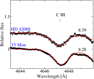
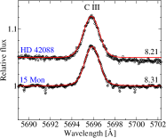
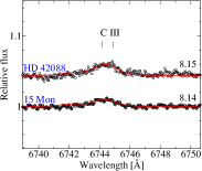
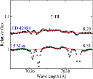
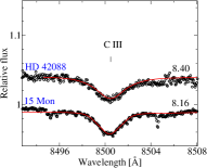
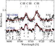
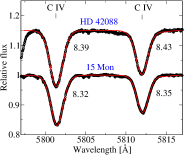
Figure 10: Best NLTE fits (solid curves) of C iii 4647, 5695, 6744, 7037, 8500, and 9701–17 Å and C iv 5801, 5811 Å in HD 42088 and 15 Mon. The observed spectra are shown by open circles.

Table 4: NLTE and LTE Carbon abundances in two O-type stars

$\lambda$ (Å )	NLTE	LTE	NLTE	LTE
	HD 42088		15 Mon
C iii
4163	8.17	8.60	–	–
4647	8.39	7.57	8.28	7.73
8500	8.40	8.63	8.16	8.63
Mean	8.33	8.46	8.22	8.38
$\sigma$	0.13	0.60	0.08	0.64
5695	8.21	$e$	8.31	$e$
6744	8.15	$e$	8.14	$e$
7037	8.29	$e$	8.31	$e$
9705–17	8.04	$e$	8.09	$e$
Mean	8.18	–	8.22	–
$\sigma$	0.11	–	0.11	–
Mean C iii	8.25	8.46	8.22	8.38
$\sigma$	0.13	0.60	0.10	0.64
C iv
5801	8.37	9.86	8.32	9.74
5811	8.41	9.72	8.35	9.56
Mean C iv	8.39	9.80	8.34	9.66
$\sigma$	0.03	0.10	0.02	0.13

Note. — Notes. Emission lines are marked by symbol $e$.

Table 5: The Carbon NLTE abundances obtained from emission and absorption lines of four ionization stages

Number	Star	Name	log $\epsilon_{\rm C}$
1	HD 209008	18 Peg	8.37$\pm$0.14
2	HD 160762	$\iota$ Her	8.46$\pm$0.11
3	HD 35912	HR 1820	8.37$\pm$0.11
4	HD 36629	HIP 26000	8.40$\pm$0.12
5	HD 35708	$o$ Tau	8.37$\pm$0.10
6	HD 3360	$\zeta$ Cas	8.40$\pm$0.16
7	HD 122980	$\chi$ Cen	8.30$\pm$0.07
8	HD 16582	$\delta$ Cet	8.37$\pm$0.16
9	HD 29248	$\nu$ Eri	8.36$\pm$0.10
10	HD 886	$\gamma$ Peg	8.40$\pm$0.11
11	HD 74575	$\alpha$ Pix	8.39$\pm$0.08
12	HD 35299	HR 1781	8.43$\pm$0.17
13	HD 36959	HR 1886	8.46$\pm$0.14
14	HD 61068	HR 2928	8.26$\pm$0.14
15	HD 36591	HR 1861	8.37$\pm$0.11
16	HD 37042	$\theta^{2}$ Ori B	8.36$\pm$0.12
17	HD 36822	$\phi^{1}$ Ori	8.29$\pm$0.13
18	HD 34816	$\lambda$ Lep	8.40$\pm$0.12
19	HD 149438	$\tau$ Sco	8.28$\pm$0.10
20	HD 36512	$\upsilon$ Ori	8.32$\pm$0.13
21	HD 47839	15 Mon AaAb	8.27$\pm$0.11
22	HD 42088		8.31$\pm$0.11

3.4 Discussions

We examine the reliability of carbon abundances obtained from C ii 4267, 9903 Å and C iii 5695 Å lines. The C ii 4267, 9903 Å lines reach a maximum strength around $T_{\rm eff}$ $\sim$21 000 and ∼30 000 K, respectively. The C iii 5695 Å line reaches a maximum strength in absorption at $T_{\rm eff}$ $=$33 400 K, and is still in emission at $T_{\rm eff}$ $=$38 000 K.

It is known from the observations of the CHANDRA satellite (Nazé et al., 2011), that the X-ray fluxes in O-B stars can be higher than theoretical one, that can lead to underestimation of radiation in the far UV and, as a result, to the underestimation of the degree of ionization, that can lead to lower abundances dependent on the temperature. Our stars have effective temperatures lying in the range 15 800–38 000 K. No trend between the abundances from C ii 4267, 6578, 6582 Å and C iii 5695 Å lines and effective temperature is apparent (Fig. 11).

The obtained abundances from C ii 4267 Å line are systematically lower by 0.20 $-$ 0.30 dex compared to other C ii lines in the stars with $T_{\rm eff}$ $\leq$ 22 000 K. The C ii 4267 Å line provides consistent abundances at the temperature range from 22 900 K to 30 000 K only, where the agreement between C ii 4267 Å and the other carbon lines is within 0.14 dex.

Other two classical strong lines of C ii 6578/82 Å show too high abundances in several of the cooler sample stars, switching to too low abundance in some of the higher temperature stars, that well demonstrated on Figure 11. However, for eight stars in our sample, $\iota$ Her, HIP 26000, $o$ Tau, $\chi$ Cen, $\alpha$ Pix, HR 1886, HR 2928, HR 1861, the discrepancies between C ii 6578 Å and other carbon lines do not exceed 0.10 dex. We have noticed that the line C ii 6578 Å shows systematically lower abundance by about 0.07 dex compared to the C ii 6582 Å in all sample stars, however both of them belong to same multiplet.

The prominent discrepancies between C ii 4267 Å and C ii 6582 Å were found in the most of the stars, except for six of them, HR 1820, $\alpha$ Pix, $\phi^{1}$ Ori, $\lambda$ Lep, $\tau$ Sco in which the value, log $\epsilon_{\rm C}(6582)$ $-$ log $\epsilon_{\rm C}(4267)$, is lower than 0.14 dex. For six stars, HR 1820, $\alpha$ Pix, HR 2928, $\theta^{2}$ Ori B, $\tau$ Sco, and $\upsilon$ Ori, the abundances from C ii 4267 Å and C ii 6578 Å are found to be consistent within 0.10 dex.

We have found that the mean abundance from emission C ii 9903 Å line in the stars with $T_{\rm eff}$$<$25 000 K is log $\epsilon_{\rm C}$=8.48$\pm$0.12, while in the stars with $T_{\rm eff}$$>$25 000 K is log $\epsilon_{\rm C}$=8.16$\pm$0.10 (Fig. 11). We find a small (within 3 $\sigma$) temperature dependence in the C abundances between hot and cool stars. The most probable reason for this apparent difference is our treatment of the model atom, in which R-matrix calculations for effective collision strengths (dependent on temperature) have been carried out only for 30 lowest fine-structure levels of C ii available in the literature.

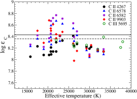
Figure 11: Carbon NLTE abundances in program stars derived from lines of C ii at 4267, 6578, 6582, and 9903 Å and of C iii at 5695 Å in a wide temperature range. The solid line represents solar value, log $\epsilon_{\rm C}$=8.43. The dashed line represents the NLTE abundance averaged over all C i, C ii and C iii lines, log $\epsilon_{\rm C}$=8.36.

3.5 Comparison with previous studies

We obtained log $\epsilon_{\rm C}$=8.36$\pm$0.08 from twenty B-type stars, that is in a good agreement with present-day Cosmic abundance standard (Nieva & Przybilla, 2012), where log $\epsilon_{\rm C}$=8.33$\pm$0.04 was obtained in twenty B-stars. It is not surprising, because the sixteen stars in our sample are common with Nieva & Przybilla (2012) and our methods of calculations are similar. However, there are some differences in the used model atom. Nieva & Przybilla (2008) performed the NLTE calculations for C ii/C iii/C iv on the basis of the ATLAS9 model atmosphere using Maxwellian-averaged collision strengths for electron-impact excitation among the lowest 24 terms of C iii from the R-matrix computations of Mitnik et al. (2003), and effective collision strengths for the lowest 24 fine-structure levels of C iv from Aggarwal & Keenan (2004). The departure coefficients computed for the atmosphere with 32 000 / 4.3, corresponding to $\tau$ Sco (Fig. 4 for the levels of C ii and C iii and Fig. 5 for C iv) are similar to departure coefficients in Nieva & Przybilla (2008). We briefly comment on some individual stars as follows.

HD 160762 ($\iota$ Her). In Alexeeva et al. (2016), the star was found to have log $\epsilon_{\rm C}$=8.43$\pm$0.10 from emission C i and absorption C ii lines (totally 20 lines), that is in agreement with this work, log $\epsilon_{\rm C}$=8.46$\pm$0.11, where we added the abundance from emission C ii 9903 Å line. Nieva & Przybilla (2012) obtained log $\epsilon_{\rm C}$=8.40$\pm$0.07 from 13 lines of C ii, that is consistent with both Alexeeva et al. (2016) and this work.

HD 36512 ($\upsilon$ Ori). In this star, we obtained log $\epsilon_{\rm C}$=8.32$\pm$0.13 from 23 lines of three ionization stages, C ii, and C iii, and C iv. Carneiro et al. (2018) derived a carbon abundance of log $\epsilon_{\rm C}$=8.25$\pm$0.22 with NLTE atmosphere code fastwind, that is slightly lower than our result, although still consistent within the error bars. Our result is consistent with Martins et al. (2015c), who obtained log $\epsilon_{\rm C}$=8.38$\pm$0.12 with the code cmfgen that computes NLTE and spherical models. Our result is in line with Nieva & Przybilla (2012), in which they obtained 8.35$\pm$0.14 from 19 lines of three ionization stages.

HD 47839 (15 Mon AaAb). 15 Monocerotis is a bright O-type star (m_V = 4.64) in a spectroscopic binary system that belongs to an open cluster NGC 2264 located at about $d$ $\approx$ 720 pc from the Sun (Cvetković et al., 2010; Maíz Apellániz, 2019). An orbital period of 25 years was estimated by Gies et al. (1993). Recent astrometric calculations based on the GAIA DR2 indicate a period of 108 years (Maíz Apellániz, 2019). The difference in magnitude between Aa and Ab is 1.2 mag (Maíz Apellániz et al., 2018), which indicates that Ab is likely to be a late-O or an early-B star, but there is no spatially separated spectroscopy to confirm that. Gies et al. (1993) showed that the broad component of He i 5876 Å line in the spectrum of the primary component can be potentially associated with the companion. For the secondary component, they estimated spectral type 09.5 V and quite a large projected rotational velocity $v$ sin $i$ = 350$\pm$40 km s^-1 based on the shape of the wings. The domination of the primary component to the line flux, in combination with such a large rotational velocity, complicates the detection of the secondary by the spectral observations. In the case of 15 Mon AaAb, we do not notice any broad features originating from the secondary in the wings of the investigated carbon lines, even in the strong C iii 5695 and C iv 5801, 5811 Å (Fig. 10). Due to the high rotational velocity of the secondary, other weak lines would be broad and shallow and almost indistinguishable from the continuum level. Even then, abundance results can be affected by the spectroscopic binarity. When the spectrum of the primary is diluted by that of the rapidly rotating secondary, spectral lines on the normalized continuum might be apparently weakened. Then, abundances obtained by assuming a single star may contain some errors. However, we are presently unable to quantify the effect of the secondary star to the normalized continuum and to estimate the resulting errors quantitatively. We obtained a carbon abundance in this star and our mean value, log $\epsilon_{\rm C}$=8.27$\pm$0.11, is lower by 0.16 dex than the solar value. We find no previous study on the carbon abundance in this star.

HD 42088. It is a Blue Straggler and a member of Gem OB1 stellar association (Schild & Berthet, 1986). It also is considered as a peculiar star with nitrogen overabundance (Schild & Berthet, 1986). The derived carbon abundance for HD 42088 ($T_{\rm eff}$ = 38 000, log $g$ = 4.0), log $\epsilon_{\rm C}$=8.31$\pm$0.11, is consistent with Martins et al. (2015c), who obtained log $\epsilon_{\rm C}$=8.30$\pm$0.06 using the code cmfgen with NLTE model including wind, line-blanketing and spherical geometry. Our line-by-line scatter is higher, because we used a different set of lines. For example, such lines as C iii 4647, 8500, 5695, 7037, 9705$-$9717 Å, and C iv 5801, 5811 Å, were not included in analysis of Martins et al. (2015c).

4 Conclusions

We present a model atom for C i–C ii–C iii–C iv using the most up-to-date atomic data and evaluated the non-local thermodynamic equilibrium (NLTE) line formation in classical 1D atmospheric models of O-B-type stars with the code detail. The model atom allows the absorption and emission lines of C i, C ii, C iii, and C iv to be analyzed in the atmospheres of O-B type stars with effective temperature 15 800 $\leq$ $T_{\rm eff}$$\leq$ 38 000 K and surface gravity 3.60 $\leq$ log $g$ $\leq$ 4.30.

Our modeling predicts the emission lines of C ii 9903 and 18 535 Å that appear at effective temperature of $T_{\rm eff}$$\geq$ 17 500 K, those of C ii 6151 and 6461 Å that appear at effective temperature of $T_{\rm eff}$$>$ 25 000 K, and the emission lines of C iii 5695, 6728–44, 9701–17 Å that appear at effective temperature of $T_{\rm eff}$$\geq$ 35 000 K (log $g$=4.0). These emission lines form in the stellar atmosphere, and NLTE effects are responsible for the formation of emission. A pre-requisite of the emission is the depletion of population in a minority species, where the photoionization-recombination mechanism provides an inversion of populations of energy levels. Our detailed analysis shows that the upper levels of the transitions at C ii 9903 and 18 535 Å are mainly populated from C iii reservoir through the Rydberg states. Photon losses in UV transitions at 885, 1308, and 1426–28 Å that become optically thin in the photosphere drive the extra depopulation of the lower levels of transitions at C iii 5695, 6728–44 Å. The upper levels of transitions at C iii 9701–17 Å are mainly populated due to spontaneous deexcitation at C iii 1577 and 1923 Å. The emission lines of C ii 6151, 6461, 9903, 18 535 Å and C iii 5695, 6728–44, 9701–17 Å in the spectra of main-sequence O-B-type stars is the result of atomic processes taking place between levels. We confirm that the emission can be obtained without the external mechanisms of excitation, the hypothesis of extended envelopes, atmospheric expansion and supplemental non-radiative influxes of energy.

We analysed the lines of C i, C ii, C iii, and C iv in twenty-two O-B-type stars with temperature range 15 800 $\leq$ $T_{\rm eff}$$\leq$ 38 000 K taking the advantages of their observed high-resolution, high SN ratio, and broad wavelength coverage spectra, where SN ratio is higher than 1000 for some of them. Stellar parameters of our stars were reliably determined by Nieva & Przybilla (2012); Nieva & Simón-Díaz (2011); Markova et al. (2004); Martins et al. (2015c). The emission line C ii 9903 Å was predicted theoretically and well-reproduced in the observations of B-stars for the first time.

We examine the reliability of carbon abundances determined from the absorption C ii line at 4267 Å and the emission line of C ii at 9903 Å in B-stars and the line C iii at 5695 Å in O-type stars. There is no hint of a trend between the abundances from C ii 4267 and C iii 5695 Å lines and effective temperature in the investigated temperature range. Although, we found a hint on the trend between the abundances from emission C ii 9903 Å line and effective temperature, where the mean abundance from C ii 9903 Å line in the stars with $T_{\rm eff}$$<$25 000 K is 8.48$\pm$0.12, while in the stars with $T_{\rm eff}$$>$25 000 K is 8.16$\pm$0.10. Though the agreement is within 3$\sigma$, we might attribute the apparent discrepancy to be due to the shortcoming of our model atom, where in the $R$-matrix calculations for effective collision strengths are not available in the literature, except for the 30 lowest fine-structure levels in C ii. The C ii 4267 Å line provides reliable abundances at the temperature range from 22 900 K to 30 000 K only, while for cooler stars, with $T_{\rm eff}$ $\leq$ 22 000 K, the abundances from C ii 4267 Å line are systematically lower by 0.20$-$0.30 dex compared to other C ii lines.

We conclude that the abundances from emission lines of C i, C ii and C iii do not differ significantly from absorption ones, that makes them potential abundance indicator as well. Consistent abundances from emission lines of C i and absorption lines of C ii have been found for $\iota$ Her, HIP 26000 and $\chi$ Cen, while for other stars, HR 1820 and $\zeta$ Cas, the agreement is still within 1$\sigma$. Consistent abundances within the error bars from C ii emission and C ii absorption lines were found in $\iota$ Her, HR 1820, $\zeta$ Cas, $\chi$ Cen, $\nu$ Eri, $\gamma$ Peg, $\alpha$ Pix, HR 1781, $\lambda$ Lep, $\tau$ Sco, and $\upsilon$ Ori. Consistent abundances within the error bars from C iii emission and C iii absorption lines were found in 15 Mon and HD 42088, however the abundance from C iii emission lineas at 9705$-$17 are systematically lower by about 0.20 dex.

For each star, NLTE leads to smaller line-to-line scatter. The NLTE must be taken into account since the deviations from LTE are strong in the investigated temperature regime. For example, in C iv lines at 5801 and 5811 Å among O-type stars, the difference between NLTE and LTE abundances, $\Delta_{\rm NLTE}$, can reach up to $-$1.49 dex. In the LTE assumption, we only can recommend the C ii 5132–5151 Å lines as carbon abundance indicator in the stars with 15 000 $\leq$ $T_{\rm eff}$$\leq$ 21 000 K, due to small NLTE effects for these lines. For stars with 26 000 $\leq$ $T_{\rm eff}$$\leq$ 32 000 K, the C iii 4056 Å line can be used in a LTE analysis. We obtained log $\epsilon_{\rm C}$=8.36$\pm$0.08 from twenty B-type stars in the solar vicinity, which is in a good agreement with a present-day Cosmic abundance standard (Nieva & Przybilla, 2012). The obtained carbon abundances in 15 Mon and HD 42088 are 8.27$\pm$0.11 and 8.31$\pm$0.11, that is lower by 0.16 dex and 0.12 dex than the solar value, respectively.

.

References

- Aggarwal & Keenan (2004) Aggarwal, K. M., & Keenan, F. P. 2004, Phys. Scr, 69, 385, doi: 10.1238/Physica.Regular.069a00385
- Alexeeva et al. (2018) Alexeeva, S., Ryabchikova, T., Mashonkina, L., & Hu, S. 2018, ApJ, 866, 153, doi: 10.3847/1538-4357/aae1a8
- Alexeeva & Mashonkina (2015) Alexeeva, S. A., & Mashonkina, L. I. 2015, MNRAS, 453, 1619, doi: 10.1093/mnras/stv1668
- Alexeeva et al. (2016) Alexeeva, S. A., Ryabchikova, T. A., & Mashonkina, L. I. 2016, MNRAS, 462, 1123, doi: 10.1093/mnras/stw1635
- Andrievsky et al. (1999) Andrievsky, S. M., Korotin, S. A., Luck, R. E., & Kostynchuk, L. Y. 1999, A&A, 350, 598
- Butler & Giddings (1985) Butler, K., & Giddings, J. 1985, Newsletter on the analysis of astronomical spectra, No. 9, University of London
- Carlsson et al. (1992) Carlsson, M., Rutten, R. J., & Shchukina, N. G. 1992, A&A, 253, 567
- Carneiro et al. (2018) Carneiro, L. P., Puls, J., & Hoffmann, T. L. 2018, A&A, 615, A4, doi: 10.1051/0004-6361/201731839
- Castelli & Hubrig (2004) Castelli, F., & Hubrig, S. 2004, A&A, 425, 263, doi: 10.1051/0004-6361:20041011
- Castelli & Hubrig (2007) —. 2007, A&A, 475, 1041, doi: 10.1051/0004-6361:20077923
- Castelli & Kurucz (2003) Castelli, F., & Kurucz, R. L. 2003, in IAU Symposium, Vol. 210, Modelling of Stellar Atmospheres. Uppsala, Sweden, 17-21 June, 2002. Published on behalf of the IAU by the Astronomical Society of the Pacific, ed. N. Piskunov, W. W. Weiss, & D. F. Gray, A20
- Cunha & Lambert (1994) Cunha, K., & Lambert, D. L. 1994, ApJ, 426, 170, doi: 10.1086/174053
- Cunto et al. (1993) Cunto, W., Mendoza, C., Ochsenbein, F., & Zeippen, C. J. 1993, Bulletin d’Information du Centre de Donnees Stellaires, 42, 39
- Cvetković et al. (2010) Cvetković, Z., Vince, I., & Ninković, S. 2010, New A, 15, 302, doi: 10.1016/j.newast.2009.09.002
- Daflon et al. (1999) Daflon, S., Cunha, K., & Becker, S. R. 1999, ApJ, 522, 950, doi: 10.1086/307683
- Daflon et al. (2001a) Daflon, S., Cunha, K., Becker, S. R., & Smith, V. V. 2001a, ApJ, 552, 309, doi: 10.1086/320460
- Daflon et al. (2004a) Daflon, S., Cunha, K., & Butler, K. 2004a, ApJ, 604, 362, doi: 10.1086/381683
- Daflon et al. (2004b) —. 2004b, ApJ, 606, 514, doi: 10.1086/382951
- Daflon et al. (2001b) Daflon, S., Cunha, K., Butler, K., & Smith, V. V. 2001b, ApJ, 563, 325, doi: 10.1086/323795
- Donati et al. (2006) Donati, J.-F., Catala, C., Landstreet, J. D., & Petit, P. 2006, in Astronomical Society of the Pacific Conference Series, Vol. 358, Solar Polarization 4, ed. R. Casini & B. W. Lites, 362
- Fernández-Menchero et al. (2014) Fernández-Menchero, L., Del Zanna, G., & Badnell, N. R. 2014, A&A, 566, A104, doi: 10.1051/0004-6361/201423864
- Gies & Lambert (1992) Gies, D. R., & Lambert, D. L. 1992, ApJ, 387, 673, doi: 10.1086/171116
- Gies et al. (1993) Gies, D. R., Mason, B. D., Hartkopf, W. I., et al. 1993, AJ, 106, 2072, doi: 10.1086/116786
- Green et al. (1957) Green, L. C., Rush, P. P., & Chandler, C. D. 1957, ApJS, 3, 37, doi: 10.1086/190031
- Griffin et al. (2000) Griffin, D. C., Badnell, N. R., & Pindzola, M. S. 2000, Journal of Physics B Atomic Molecular Physics, 33, 1013, doi: 10.1088/0953-4075/33/5/315
- Hibbert et al. (1993) Hibbert, A., Biemont, E., Godefroid, M., & Vaeck, N. 1993, A&AS, 99, 179
- Hillier & Miller (1998) Hillier, D. J., & Miller, D. L. 1998, ApJ, 496, 407, doi: 10.1086/305350
- Holgado et al. (2018) Holgado, G., Simón-Díaz, S., Barbá, R. H., et al. 2018, A&A, 613, A65, doi: 10.1051/0004-6361/201731543
- Hubrig & González (2007) Hubrig, S., & González, J. F. 2007, A&A, 466, 1083, doi: 10.1051/0004-6361:20066738
- Hunter et al. (2009) Hunter, I., Brott, I., Langer, N., et al. 2009, A&A, 496, 841, doi: 10.1051/0004-6361/200809925
- Kilian (1992) Kilian, J. 1992, A&A, 262, 171
- Kochukhov (2010) Kochukhov, O. 2010, BinMag IDL widget Code v6.2. Available at: http://www.astro.uu.se/oleg/
- Kochukhov (2018) —. 2018, BinMag: Widget for comparing stellar observed with theoretical spectra, Astrophysics Source Code Library. http://ascl.net/1805.015
- Kramida et al. (2018) Kramida, A., Ralchenko, Yu., Reader, J., & NIST ASD Team. 2018, NIST Atomic Spectra Database (ver. 5.5.2), [Online]. Available: https://physics.nist.gov/asd [2018, January 25]. National Institute of Standards and Technology, Gaithersburg, MD.
- Kupka et al. (1999) Kupka, F., Piskunov, N., Ryabchikova, T. A., Stempels, H. C., & Weiss, W. W. 1999, A&AS, 138, 119, doi: 10.1051/aas:1999267
- Luo et al. (1989) Luo, D., Pradhan, A. K., Saraph, H. E., Storey, P. J., & Yu, Y. 1989, Journal of Physics B Atomic Molecular Physics, 22, 389, doi: 10.1088/0953-4075/22/3/006
- Lyubimkov et al. (2013) Lyubimkov, L. S., Lambert, D. L., Poklad, D. B., Rachkovskaya, T. M., & Rostopchin, S. I. 2013, MNRAS, 428, 3497, doi: 10.1093/mnras/sts287
- Maíz Apellániz (2019) Maíz Apellániz, J. 2019, arXiv e-prints, arXiv:1908.02040. https://arxiv.org/abs/1908.02040
- Maíz Apellániz et al. (2018) Maíz Apellániz, J., Barbá, R. H., Simón-Díaz, S., et al. 2018, A&A, 615, A161, doi: 10.1051/0004-6361/201832885
- Markova et al. (2004) Markova, N., Puls, J., Repolust, T., & Markov, H. 2004, A&A, 413, 693, doi: 10.1051/0004-6361:20031463
- Martins & Hillier (2012) Martins, F., & Hillier, D. J. 2012, A&A, 545, A95, doi: 10.1051/0004-6361/201219788
- Martins et al. (2017) Martins, F., Simón-Díaz, S., Barbá, R. H., Gamen, R. C., & Ekström, S. 2017, A&A, 599, A30, doi: 10.1051/0004-6361/201629548
- Martins et al. (2015a) Martins, F., Simón-Díaz, S., Palacios, A., et al. 2015a, A&A, 578, A109, doi: 10.1051/0004-6361/201526130
- Martins et al. (2015b) Martins, F., Hervé, A., Bouret, J. C., et al. 2015b, A&A, 575, A34, doi: 10.1051/0004-6361/201425173
- Martins et al. (2015c) Martins, F., Hervé, A., Bouret, J.-C., et al. 2015c, A&A, 575, A34, doi: 10.1051/0004-6361/201425173
- Mitnik et al. (2003) Mitnik, D. M., Griffin, D. C., Ballance, C. P., & Badnell, N. R. 2003, Journal of Physics B Atomic Molecular Physics, 36, 717, doi: 10.1088/0953-4075/36/4/306
- Nahar (1995) Nahar, S. N. 1995, ApJS, 101, 423, doi: 10.1086/192248
- Nahar & Pradhan (1997) Nahar, S. N., & Pradhan, A. K. 1997, ApJS, 111, 339, doi: 10.1086/313013
- Nazé et al. (2011) Nazé, Y., Broos, P. S., Oskinova, L., et al. 2011, ApJS, 194, 7, doi: 10.1088/0067-0049/194/1/7
- Nieva & Przybilla (2006) Nieva, M. F., & Przybilla, N. 2006, ApJ, 639, L39, doi: 10.1086/501124
- Nieva & Przybilla (2007) —. 2007, A&A, 467, 295, doi: 10.1051/0004-6361:20065757
- Nieva & Przybilla (2008) —. 2008, A&A, 481, 199, doi: 10.1051/0004-6361:20078203
- Nieva & Przybilla (2012) Nieva, M.-F., & Przybilla, N. 2012, A&A, 539, A143, doi: 10.1051/0004-6361/201118158
- Nieva & Simón-Díaz (2011) Nieva, M.-F., & Simón-Díaz, S. 2011, A&A, 532, A2, doi: 10.1051/0004-6361/201116478
- Osorio et al. (2015) Osorio, Y., Barklem, P. S., Lind, K., et al. 2015, A&A, 579, A53, doi: 10.1051/0004-6361/201525846
- Przybilla et al. (2011) Przybilla, N., Nieva, M.-F., & Butler, K. 2011, Journal of Physics Conference Series, 328, 012015, doi: 10.1088/1742-6596/328/1/012015
- Puls et al. (2005) Puls, J., Urbaneja, M. A., Venero, R., et al. 2005, A&A, 435, 669, doi: 10.1051/0004-6361:20042365
- Ryabchikova et al. (2016) Ryabchikova, T., Piskunov, N., Pakhomov, Y., et al. 2016, MNRAS, 456, 1221, doi: 10.1093/mnras/stv2725
- Rybicki & Hummer (1991) Rybicki, G. B., & Hummer, D. G. 1991, A&A, 245, 171
- Ryde et al. (2004) Ryde, N., Korn, A. J., Richter, M. J., & Ryde, F. 2004, ApJ, 617, 551, doi: 10.1086/425265
- Sadakane & Nishimura (2017) Sadakane, K., & Nishimura, M. 2017, PASJ, 69, 48, doi: 10.1093/pasj/psx024
- Sadakane & Nishimura (2019) —. 2019, PASJ, 71, 45, doi: 10.1093/pasj/psz016
- Sadakane et al. (2001) Sadakane, K., Takada-Hidai, M., Takeda, Y., et al. 2001, PASJ, 53, 1223, doi: 10.1093/pasj/53.6.1223
- Sakhibullin et al. (1982) Sakhibullin, N. A., Auer, L. H., & van der Hucht, K. 1982, Soviet Ast., 26, 563
- Schild & Berthet (1986) Schild, H., & Berthet, S. 1986, A&A, 162, 369
- Seaton (1962) Seaton, M. J. 1962, in Atomic and Molecular Processes, Academic Press Inc., U.S., ed. D. R. Bates, 375
- Sigut (1996) Sigut, T. A. A. 1996, ApJ, 473, 452, doi: 10.1086/178157
- Sigut (2001a) —. 2001a, A&A, 377, L27, doi: 10.1051/0004-6361:20011211
- Sigut (2001b) —. 2001b, ApJ, 546, L115, doi: 10.1086/318870
- Sigut et al. (2000) Sigut, T. A. A., Landstreet, J. D., & Shorlin, S. L. S. 2000, ApJ, 530, L89, doi: 10.1086/312499
- Simón-Díaz et al. (2017) Simón-Díaz, S., Godart, M., Castro, N., et al. 2017, A&A, 597, A22, doi: 10.1051/0004-6361/201628541
- Sitnova et al. (2018) Sitnova, T. M., Mashonkina, L. I., & Ryabchikova, T. A. 2018, MNRAS, 477, 3343, doi: 10.1093/mnras/sty810
- Sundqvist et al. (2008) Sundqvist, J. O., Ryde, N., Harper, G. M., Kruger, A., & Richter, M. J. 2008, A&A, 486, 985, doi: 10.1051/0004-6361:200809778
- van Regemorter (1962) van Regemorter, H. 1962, ApJ, 136, 906, doi: 10.1086/147445
- Wahlgren & Hubrig (2000) Wahlgren, G. M., & Hubrig, S. 2000, A&A, 362, L13
- Wahlgren & Hubrig (2004) —. 2004, A&A, 418, 1073, doi: 10.1051/0004-6361:20034257
- Walborn (1980) Walborn, N. R. 1980, ApJS, 44, 535, doi: 10.1086/190704
- Wilson et al. (2005) Wilson, N. J., Bell, K. L., & Hudson, C. E. 2005, A&A, 432, 731, doi: 10.1051/0004-6361:20041855