The exact solution of a generalized two-spins model

G. Santos

Universidade Federal de Sergipe - UFS

Centro de Ciências Exatas e Tecnologia - CCET

Departamento de Física

Cidade Univ. Prof. José Aloísio de Campos

Av. Marechal Rondon, s/n, Jd. Rosa Elze

São Cristóvão/SE - Brazil.

gnsfilho@gmail.com

Abstract

We present the exact solution of a family of two-spins models. The models are solved by the algebraic Bethe ansatz method using the $gl(2)$-invariant $R$-matrix and a multi-spins Lax operator. The interactions are by the Heisenberg spins exchange. We are also considering magnetic $B$-fields and a term for Haldane single spin anisotropy.

1 Introduction

The algebraic formulation of the Bethe ansatz method, and the associated quantum inverse scattering method (QISM), was primarily developed in [1, 2, 3, 4, 5] and it has been used to study a considerable number of exactly solvable systems, such as, one-dimensional spin chains, quantum field theory of one-dimensional interacting bosons [6] and fermions [7], two-dimensional lattice models [8], systems of strongly correlated electrons [9, 10], conformal field theory [11], integrable systems in high energy physics [12, 13, 14, 15, 16, 17] and quantum algebras [18, 19, 20, 21]. More recently solvable models have also shown up in relation to string theories [22, 23, 24]. Remarkably it is important to mention that exactly solvable models are recently finding their way into the lab, mainly in the context of ultracold atoms [25, 26, 27, 28, 29, 30, 31] but also in nuclear magnetic resonance (NMR) experiments[32, 33] becoming its study as well as the derivation of new models an even more fascinating field. We are considering in this work a multi-spins Lax operator that like the multi-bosons Lax operator in [34] permits to solve a family of models, helping to increase the number of integrable models solved by the algebraic Bethe ansatz method. These spins cluster integrable models are important as for example in quantum computation and quantum information, quantum simulation using nuclear magnetic resonance (NMR) [35, 36, 37] or trapped ions [38] as well as in molecular magnetism [39]. Recently, spins configurations like these were proposed in [38] to a universal digital quantum simulation with trapped ions and an experimental realization of the Yang-Baxter equation was realized via NMR interferometry [32] using Iodotrifluoroethylene $(C_{2}F_{3}I)$ molecules. Another important application of this spins configurations is as a spin network that appears in quantum gravity [40, 41].

The paper is organized as follows. In section 2, I will describe briefly the algebraic Bethe ansatz method and present the multi-spins Lax operators. In section 3, I present a generalized two-spins model. In section 4, I present the exact solution. In section 5, I summarize the results.

2 Algebraic Bethe ansatz method

In this section we will shortly describe the algebraic Bethe ansatz method and present the Lax operators used to get the solution of the models [43, 42]. We begin with the $gl(2)$-invariant $R$-matrix, depending on the spectral parameter $u$,

$$R(u)=\left(\begin{array}[]{cccc}1&0&0&0\\ 0&b(u)&c(u)&0\\ 0&c(u)&b(u)&0\\ 0&0&0&1\end{array}\right),$$ (2.1)

with $b(u)=u/(u+\eta)$, $c(u)=\eta/(u+\eta)$ and $b(u)+c(u)=1$. Above, $\eta$ is an arbitrary parameter, to be chosen later.

It is easy to check that $R(u)$ satisfies the Yang-Baxter equation

$$R_{12}(u-v)R_{13}(u)R_{23}(v)=R_{23}(v)R_{13}(u)R_{12}(u-v),$$ (2.2)

where $R_{jk}(u)$ denotes the matrix acting non-trivially on the $j$-th and the $k$-th spaces and as the identity on the remaining space.

Next we define the monodromy matrix $\hat{T}(u)$,

$$\hat{T}(u)=\left(\begin{array}[]{cc}\hat{A}(u)&\hat{B}(u)\\ \hat{C}(u)&\hat{D}(u)\end{array}\right),$$ (2.3)

such that the Yang-Baxter algebra is satisfied

$$R_{12}(u-v)\hat{T}_{1}(u)\hat{T}_{2}(v)=\hat{T}_{2}(v)\hat{T}_{1}(u)R_{12}(u-v).$$ (2.4)

In what follows we will choose a realization for the monodromy matrix $\pi(\hat{T}(u))=\hat{L}(u)$ to obtain the solutions of a family of two-spins models. In this construction, the Lax operators $\hat{L}(u)$ have to satisfy the relation

$$R_{12}(u-v)\hat{L}_{1}(u)\hat{L}_{2}(v)=\hat{L}_{2}(v)\hat{L}_{1}(u)R_{12}(u-v).$$ (2.5)

Then, defining the transfer matrix, as usual, through

$$\hat{t}(u)=tr\;\pi(\hat{T}(u))=\pi(\hat{A}(u)+\hat{D}(u)),$$ (2.6)

it follows from (2.4) that the transfer matrix commutes for different values of the spectral parameter; i. e.,

$$[\hat{t}(u),\hat{t}(v)]=0,\;\;\;\;\;\;\;\forall\;u,\;v.$$ (2.7)

Consequently, the models derived from this transfer matrix will be integrable. Another consequence is that the coefficients $\hat{\mathcal{C}}_{k}$ in the transfer matrix $\hat{t}(u)$,

$$\hat{t}(u)=\sum_{k}\hat{\mathcal{C}}_{k}u^{k},$$ (2.8)

are conserved quantities or simply $c$-numbers, with

$$[\hat{\mathcal{C}}_{j},\hat{\mathcal{C}}_{k}]=0,\;\;\;\;\;\;\;\forall\;j,\;k.$$ (2.9)

If the transfer matrix $\hat{t}(u)$ is a polynomial function in $u$, with $k\geq 0$, it is easy to see that,

$$\hat{\mathcal{C}}_{0}=\hat{t}(0)\;\;\;\mbox{and}\;\;\;\hat{\mathcal{C}}_{k}=\frac{1}{k!}\left.\frac{d^{k}\hat{t}(u)}{du^{k}}\right|_{u=0}.$$ (2.10)

For the standard $SU(2)$ spin operators satisfying the commutation relations

$$[\hat{S}_{pj}^{+},\hat{S}_{qk}^{-}]=2\;\delta_{jk}\;\delta_{pq}\;\hat{S}_{kq}^{z},\qquad[\hat{S}_{pj}^{z},\hat{S}_{qk}^{\pm}]=\pm\;\delta_{jk}\;\delta_{pq}\;\hat{S}_{kq}^{\pm},$$ (2.11)

$$[\hat{\vec{S}}_{pj}^{2},\hat{S}_{qk}^{\pm}]=0,$$ (2.12)

with $p,q=a\;\mbox{or}\;b$, $j=1,\ldots,n$ and $k=1,\ldots,m$, we have the following Lax operators,

$$\hat{L}^{S_{a}^{n}}(u)=\left(\begin{array}[]{cc}\gamma_{a}u\hat{I}-\eta\sum_{j=1}^{n}\gamma_{a}\hat{S}_{aj}^{z}&-\eta\sum_{j=1}^{n}\alpha_{aj}\hat{S}_{aj}^{+}\\ -\eta\sum_{j=1}^{n}\beta_{aj}\hat{S}_{aj}^{-}&\rho_{a}u\hat{I}+\eta\sum_{j=1}^{n}\rho_{a}\hat{S}_{aj}^{z}\end{array}\right),$$ (2.13)

$$\hat{L}^{S_{b}^{m}}(u)=\left(\begin{array}[]{cc}\gamma_{b}u\hat{I}-\eta\sum_{k=1}^{m}\gamma_{b}\hat{S}_{bk}^{z}&-\eta\sum_{k=1}^{m}\alpha_{bk}\hat{S}_{bk}^{+}\\ -\eta\sum_{k=1}^{m}\beta_{bk}\hat{S}_{bk}^{-}&\rho_{b}u\hat{I}+\eta\sum_{k=1}^{m}\rho_{b}\hat{S}_{bk}^{z}\end{array}\right),$$ (2.14)

with the condition $\alpha_{aj}\beta_{aj}=\gamma_{a}\rho_{a}$ and $\alpha_{bk}\beta_{bk}=\gamma_{b}\rho_{b},\;\;\forall\;j,\;k$. The above Lax operators satisfies the equation (2.5).

3 Generalized two-spins model

In this section I present the generalized two-spins model with two different spins: $a$ and $b$. The Hamiltonian is,

$$\hat{H} = \sum_{j=1}^{n}B^{z}_{aj}\hat{S}^{z}_{aj}+\sum_{k=1}^{m}B^{z}_{bk}\hat{S}^{z}_{bk}+\sum_{j=1}^{n}D_{aj}(\hat{S}_{aj}^{z})^{2}+\sum_{k=1}^{m}D_{bk}(\hat{S}^{z}_{bk})^{2}$$ (3.15)

$$+ \sum_{i=1}^{n}\sum_{j\neq i}^{n}J^{z}_{aiaj}\hat{S}^{z}_{ai}\hat{S}^{z}_{aj}+\sum_{k=1}^{m}\sum_{l\neq k}^{m}J^{z}_{bkbl}\hat{S}^{z}_{bk}\hat{S}^{z}_{bl}$$

$$+ \sum_{j=1}^{n}\sum_{k=1}^{m}J^{z}_{ajbk}\hat{S}^{z}_{aj}\hat{S}^{z}_{bk}+\frac{1}{2}\sum_{j=1}^{n}\sum_{k=1}^{m}J^{xy}_{ajbk}(\hat{S}^{+}_{aj}\hat{S}^{-}_{bk}+\hat{S}^{-}_{aj}\hat{S}^{+}_{bk}).$$

The parameters $B^{z}_{aj}$ and $B^{z}_{bk}$ are magnetic fields in the $z$-direction, $J^{z}_{aiaj}$ are the exchange interaction parameters between the spins $a$ and $J^{z}_{bkbl}$ are the exchange interaction parameters between the spins $b$, $J^{z}_{ajbk}$ are the exchange interaction parameters between the spins $a$ and $b$ in the $z$-direction and $J^{xy}_{ajbk}\equiv J^{x}_{ajbk}=J^{y}_{ajbk}$ are the exchange interaction parameters between the spins $aj$ and $bk$ in the $x$ and $y$-direction, and $D_{aj}$ and $D_{bk}$ are the Haldane single spin anisotropy parameters for the spins $aj$ and for the spins $bk$, respectively [39].

The spins operators satisfies the $O(3)$ algebra, with the following commutation relations

$$[\hat{S}^{r}_{pj},\hat{S}^{s}_{qk}]=i\hbar\delta_{pq}\delta_{jk}\varepsilon_{rst}\hat{S}^{t}_{qk},$$ (3.16)

with $\varepsilon_{rst}$ the completely antisymmetric Levi-Civita tensor, $p,q=a,\;b$ the two spins labels, $r,s,t=x,y,z$ the spin components and $j=1\ldots n$, $k=1\ldots m$. Using the rising and the lowing operators $\hat{S}^{\pm}$ we get the commutation relations in (2.11) e (2.12)

$$\hat{S}^{\pm}_{pj}=\hat{S}^{x}_{pj}\pm i\hat{S}^{y}_{pj}.$$ (3.17)

The total spin is

$$\hat{\vec{S}}_{T}=\sum_{j=1}^{n}\hat{\vec{S}}_{aj}+\sum_{k=1}^{m}\hat{\vec{S}}_{bk},$$ (3.18)

with

$$\hat{\vec{S}}_{T}^{2}=\sum_{i,j=1}^{n}\hat{\vec{S}}_{ai}\cdot\hat{\vec{S}}_{aj}+\sum_{k,l=1}^{m}\hat{\vec{S}}_{bk}\cdot\hat{\vec{S}}_{bl}+2\sum_{i=x,y,z}\sum_{j=1}^{n}\sum_{k=1}^{m}\hat{S}^{i}_{aj}\hat{S}^{i}_{bk}.$$ (3.19)

The $z$-component of the total spin operator, $\hat{S}_{T}^{z}$,

$$\hat{S}_{T}^{z}=\sum_{j=1}^{n}\hat{S}^{z}_{aj}+\sum_{k=1}^{m}\hat{S}^{z}_{bk},$$ (3.20)

with

$$(\hat{S}_{T}^{z})^{2}=\sum_{i,j=1}^{n}\hat{S}^{z}_{ai}\hat{S}^{z}_{aj}+\sum_{k,l=1}^{m}\hat{S}^{z}_{bk}\hat{S}^{z}_{bl}+2\sum_{j=1}^{n}\sum_{k=1}^{m}\hat{S}^{z}_{aj}\hat{S}^{z}_{bk},$$ (3.21)

is a conserved quantity, $[\hat{H},\hat{S}_{T}^{z}]$.

We can represent the spins configurations of the Hamiltonian (3.15) as a complete graph $K_{s}$ (or universal graph) [44], where $s=n+m$ is the number of vertices (spins). In Fig. (1) we show the $K_{8}$ graph for the $8$-spins interaction. The number of edges (interactions) is

$$\left(\begin{tabular}[]{c}s\\ 2\\ \end{tabular}\right)=\frac{s(s-1)}{2}.$$ (3.22)

This complete graph looks like a spin network in quantum gravity [40, 41] but this full coupling network will in practice always be limited in size, as physical interactions tend to decrease with the distance. The complete graphs are also the complete $s$-partite graph $K_{s\times 1}$. If $J^{z}_{aiaj}=J^{z}_{bkbl}=D_{aj}=D_{bk}=0$ it becames the complete bipartite graph $K_{n,m}$.

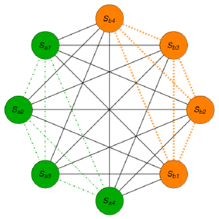
Figure 1: The complete graph $K_{8}$ showing the interactions between the spins for $n=m=4$ in the Hamiltonian (3.15). The green dashed-dotted lines stand for interaction between the spins $a$, the orange dashed lines stand for interaction between the spins $b$, and the black lines stand for interaction between the spins $a$ and the spins $b$.

In Fig. (2) we show some of the spin configurations. These small spin configurations can be considered as interaction of the nuclear spin of the atoms in a molecule, as in nuclear magnetic resonance, can be considered as plaquettes of a spin ladders or can be considered as a cell of a 3D lattice.

(a)	(b)
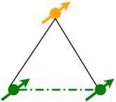
(c)	(d)

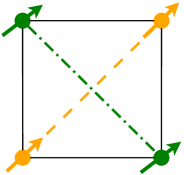
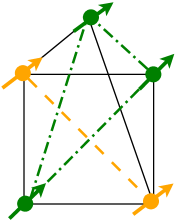
Figure 2: Some spin configuration for the generalized two-spins model with $n$ spin $a$ and $m$ spin $b$. The full black lines means interaction between the spins $a$ (green) and the spins $b$ (orange). The green dashed-dotted lines means interaction between the spins $a$ and the orange dashed line means interaction between the spins $b$. $(a)$ 1 spin $a$ and 1 spin $b$. $(b)$ 2 spin $a$ and 1 spin $b$. $(c)$ 2 spin $a$ and 2 spin $b$. $(d)$ 3 spin $a$ and 2 spin $b$.

4 Exact solution

Now we use the co-multiplication property of the Lax operators to write

$$\hat{L}(u)=\hat{L}_{1}^{S_{a}^{n}}(u+\omega_{a})\hat{L}_{2}^{S_{b}^{m}}(u-\omega_{b}).$$ (4.23)

Following the monodromy matrix (2.3) we can write the operators,

$$\pi(\hat{A}(u)) = \left(\gamma_{a}u\hat{I}+\gamma_{a}\omega_{a}\hat{I}-\eta\sum_{j=1}^{n}\gamma_{a}\hat{S}^{z}_{aj}\right)\left(\gamma_{b}u\hat{I}-\gamma_{b}\omega_{b}\hat{I}-\eta\sum_{k=1}^{m}\gamma_{b}\hat{S}^{z}_{bk}\right)$$ (4.24)

$$+ \eta^{2}\sum_{j=1}^{n}\sum_{k=1}^{m}\alpha_{aj}\beta_{bk}\hat{S}^{+}_{aj}\hat{S}_{bk}^{-},$$

$$\pi(\hat{B}(u)) = \left(\gamma_{a}u\hat{I}+\gamma_{a}\omega_{a}\hat{I}-\eta\sum_{j=1}^{n}\gamma_{a}\hat{S}^{z}_{aj}\right)\left(-\eta\sum_{k=1}^{m}\alpha_{bk}\hat{S}^{+}_{bk}\right)$$ (4.25)

$$+ \left(-\eta\sum_{j=1}^{n}\alpha_{aj}\hat{S}^{+}_{aj}\right)\left(\rho_{b}u\hat{I}-\rho_{b}\omega_{b}\hat{I}+\eta\sum_{k=1}^{m}\rho_{b}\hat{S}^{z}_{bk}\right),$$

$$\pi(\hat{C}(u)) = \left(-\eta\sum_{j=1}^{n}\beta_{aj}\hat{S}^{-}_{aj}\right)\left(\gamma_{b}u\hat{I}-\gamma_{b}\omega_{b}\hat{I}-\eta\sum_{k=1}^{m}\gamma_{b}\hat{S}^{z}_{bk}\right)$$ (4.26)

$$+ \left(\rho_{a}u\hat{I}+\rho_{a}\omega_{a}\hat{I}+\eta\sum_{j=1}^{n}\rho_{a}\hat{S}^{z}_{aj}\right)\left(-\eta\sum_{k=1}^{m}\beta_{bk}\hat{S}^{-}_{bk}\right),$$

$$\pi(\hat{D}(u)) = \left(\rho_{a}u\hat{I}+\rho_{a}\omega_{a}\hat{I}+\eta\sum_{j=1}^{n}\rho_{a}\hat{S}^{z}_{aj}\right)\left(\rho_{b}u\hat{I}-\rho_{b}\omega_{b}\hat{I}+\eta\sum_{k=1}^{m}\rho_{b}\hat{S}^{z}_{bk}\right)$$ (4.27)

$$+ \eta^{2}\sum_{j=1}^{n}\sum_{k=1}^{m}\alpha_{bk}\beta_{aj}\hat{S}^{-}_{aj}\hat{S}_{bk}^{+}.$$

Taking the trace of the operator (4.23) we get the transfer matrix

$$\hat{t}(u) = u^{2}\sigma_{ab}\hat{I}+u\sigma_{ab}\Omega_{a-b}\hat{I}-u\eta\Delta_{ab}\hat{S}^{z}_{T}-\sigma_{ab}\Xi_{a\times b}\hat{I}$$ (4.28)

$$+ \eta\Delta_{ab}\omega_{b}\sum_{j=1}^{n}\hat{S}_{aj}^{z}-\eta\Delta_{ab}\omega_{a}\sum_{k=1}^{m}\hat{S}_{bk}^{z}+\eta^{2}\sigma_{ab}\sum_{j=1}^{n}\sum_{k=1}^{m}\hat{S}_{aj}^{z}\hat{S}_{bk}^{z}$$

$$+ \eta^{2}\sum_{j=1}^{n}\sum_{k=1}^{m}\left(\alpha_{aj}\beta_{bk}\hat{S}^{+}_{aj}\hat{S}_{bk}^{-}+\alpha_{bk}\beta_{aj}\hat{S}^{-}_{aj}\hat{S}_{bk}^{+}\right),$$

where $\sigma_{ab}\equiv\gamma_{a}\gamma_{b}+\rho_{a}\rho_{b}$, $\Delta_{ab}\equiv\gamma_{a}\gamma_{b}-\rho_{a}\rho_{b}$, $\Omega_{a-b}=\omega_{a}-\omega_{b}$, $\Xi_{a\times b}=\omega_{b}\omega_{b}$.

From (2.10) we identify the conserved quantities of the transfer matrix (4.28),

$$\hat{\mathcal{C}}_{0} = -\sigma_{ab}\Xi_{a\times b}\hat{I}+\eta\Delta_{ab}\omega_{b}\sum_{j=1}^{n}\hat{S}_{aj}^{z}-\eta\Delta_{ab}\omega_{a}\sum_{k=1}^{m}\hat{S}_{bk}^{z}$$ (4.29)

$$+ \eta^{2}\sigma_{ab}\sum_{j=1}^{n}\sum_{k=1}^{m}\hat{S}_{aj}^{z}\hat{S}_{bk}^{z}+\eta^{2}\sum_{j=1}^{n}\sum_{k=1}^{m}\left(\alpha_{aj}\beta_{bk}\hat{S}^{+}_{aj}\hat{S}_{bk}^{-}+\alpha_{bk}\beta_{aj}\hat{S}^{-}_{aj}\hat{S}_{bk}^{+}\right),$$

$$\hat{\mathcal{C}}_{1} = \sigma_{ab}\Omega_{a-b}\hat{I}-\eta\Delta_{ab}\hat{S}^{z}_{T},$$ (4.30)

$$\hat{\mathcal{C}}_{2} = \sigma_{ab}\hat{I}.$$ (4.31)

We can rewrite the Hamiltonian (3.15) using these conserved quantities,

$$\hat{H}=\xi_{0}\hat{\mathcal{C}}_{0}+\hat{\mathcal{C}}_{1}(1+\xi_{1}\hat{\mathcal{C}}_{1})-\xi_{2}\hat{\mathcal{C}}_{2},$$ (4.32)

with the following identification for the parameters

$$\xi_{2}=\Omega_{a-b}(1+\xi_{1}\sigma_{ab}\Omega_{a-b})-\xi_{0}\Xi_{a\times b},$$ (4.33)

$$B^{z}_{aj}=\eta\Delta_{ab}\left(\xi_{0}\omega_{b}-2\xi_{1}\sigma_{ab}\Omega_{a-b}-1\right),$$ (4.34)

$$B^{z}_{bk}=-\eta\Delta_{ab}\left(\xi_{0}\omega_{a}+2\xi_{1}\sigma_{ab}\Omega_{a-b}+1\right),$$ (4.35)

$$D_{aj}=\xi_{1}\eta^{2}\Delta_{ab}^{2},$$ (4.36)

$$D_{bk}=\xi_{1}\eta^{2}\Delta_{ab}^{2},$$ (4.37)

$$J^{z}_{aiaj}=2\xi_{1}\eta^{2}\Delta_{ab}^{2},$$ (4.38)

$$J^{z}_{bkbl}=2\xi_{1}\eta^{2}\Delta_{ab}^{2},$$ (4.39)

$$J^{z}_{ajbk}=\eta^{2}(\xi_{0}\sigma_{ab}+2\xi_{1}\Delta_{ab}^{2}),$$ (4.40)

$$J^{xy}_{ajbk}=2\xi_{0}\eta^{2}\alpha_{aj}\beta_{bk}=2\xi_{0}\eta^{2}\alpha_{bk}\beta_{aj}.$$ (4.41)

In the Eqs. (4.38) and (4.39) we consider $i\neq j$ and $k\neq l$. Using the Eq. (4.41) and the condition $\alpha_{aj}\beta_{aj}=\alpha_{bk}\beta_{bk}$ $(\gamma_{a}\rho_{a}=\gamma_{b}\rho_{b})$ we get the following relation for the parameters $\sigma_{ab}$ and $\Delta_{ab}$,

$$\sigma_{ab}=\frac{\rho_{b}}{\rho_{a}}(\gamma_{b}^{2}+\rho_{a}^{2}),\qquad\Delta_{ab}=\frac{\rho_{b}}{\rho_{a}}(\gamma_{b}^{2}-\rho_{a}^{2}).$$ (4.42)

The $\xi_{0}$, $\gamma^{\prime}$s and $\rho^{\prime}$s parameters are arbitrary, but different of zero. The $\xi_{1}$ parameter can be zero and in this case we take out the terms with anisotropy parameter, the term with the interactions between the spins $a$ and the term with interactions between the spins $b$. We also can use $\gamma_{b}^{2}=\rho_{a}^{2}$ to cancel these interactions and turn off the $B$-field. The $\omega^{\prime}$s parameters are completely arbitrary.

The Hamiltonians (3.15) and (4.32) are related to the transfer matrix (4.28) by the equation,

$$\hat{H}=\xi_{0}\hat{t}(0)+\hat{t}^{\prime}(0)[1+\xi_{1}\hat{t}^{\prime}(0)]-\xi_{2}\hat{t}^{\prime\prime}(0),$$ (4.43)

where the prime symbol $(^{\prime})$ stand for derivatives of $\hat{t}(u)$.

We use as pseudo-vacuum the product state,

$$|0\rangle_{ajbk}=\left(\bigotimes_{j=1}^{n}|\uparrow_{z}\rangle_{aj}\right)\otimes\left(\bigotimes_{k=1}^{m}|\uparrow_{z}\rangle_{bk}\right),$$ (4.44)

with $|\uparrow_{z}\rangle_{aj}$ denoting the vacuum state for the spins $aj$ and $|\uparrow_{z}\rangle_{bk}$ denoting the vacuum state for the spins $bk$, for $j=1,\ldots,n$ and $k=1\ldots,m$. For this pseudo-vacuum we can apply the algebraic Bethe ansatz method in order to find the Bethe ansatz equations (BAEs),

$$\frac{\gamma_{a}\gamma_{b}\left(v_{i}+\omega_{a}-\eta M^{z}_{a}\right)\left(v_{i}-\omega_{b}-\eta M^{z}_{b}\right)}{\rho_{a}\rho_{b}\left(v_{i}+\omega_{a}+\eta M^{z}_{a}\right)\left(v_{i}-\omega_{b}+\eta M^{z}_{b}\right)} = \prod_{j\neq i}^{N}\frac{v_{i}-v_{j}-\eta}{v_{i}-v_{j}+\eta},\;\;\;\;\;i,j=1,\ldots,N,$$

where

$$M^{z}_{a}=\sum_{j=1}^{n}m^{z}_{aj},\qquad M^{z}_{b}=\sum_{k=1}^{m}m^{z}_{bk},$$ (4.46)

are the total magnetic moment in the $z$-direction of the respective spins $a$ and $b$.

If we choose $\omega_{a}=\omega_{b}=0$, $\gamma_{b}=\rho_{a}$ and $M^{z}_{a}=M^{z}_{b}\equiv M^{z}$ we get the BAE’s

$$\left(\frac{v_{i}-\eta M^{z}}{v_{i}+\eta M^{z}}\right)^{2} = \prod_{j\neq i}^{N}\frac{v_{i}-v_{j}-\eta}{v_{i}-v_{j}+\eta},\;\;\;\;\;i,j=1,\ldots,N.$$ (4.47)

The eigenvectors [45] $\{|v_{1},v_{2},\ldots,v_{N}\rangle\}$ of the Hamiltonian (3.15) or (4.32) and of the transfer matrix (4.28) are

$$|\vec{v}\rangle\equiv|v_{1},v_{2},\ldots,v_{N}\rangle=\prod_{i=1}^{N}\pi(\hat{C}(v_{i}))|0\rangle,$$ (4.48)

and the eigenvalues of the Hamiltonian (3.15) or (4.32) are,

$$E(\{v_{i}\}) = \xi_{0}\;\gamma_{a}\gamma_{b}\left(v_{i}+\omega_{a}-\eta M^{z}_{a}\right)\left(v_{i}-\omega_{b}-\eta M^{z}_{b}\right)\prod_{i=1}^{N}\frac{v_{i}+\eta}{v_{i}}$$ (4.49)

$$+ \xi_{0}\;\rho_{a}\rho_{b}\left(v_{i}+\omega_{a}+\eta M^{z}_{a}\right)\left(v_{i}-\omega_{b}+\eta M^{z}_{b}\right)\prod_{i=1}^{N}\frac{v_{i}-\eta}{v_{i}}$$

$$- \eta\Delta_{ab}\left(1+2\xi_{1}\;\sigma_{ab}\Omega_{a-b}\right)\left(M^{z}_{a}+M^{z}_{b}\right)$$

$$+ \xi_{1}\;\eta^{2}\Delta_{ab}^{2}\left[(M^{z}_{a})^{2}+2M^{z}_{a}M^{z}_{b}+(M^{z}_{b})^{2}\right]+\xi_{0}\sigma_{ab}\Xi_{a\times b},$$

where the $\{v_{i}\}$ are solutions of the BAEs (LABEL:BAE2).

5 Summary

We have solved a generalized two-spins model by the algebraic Bethe ansatz method using the $gl(2)$-invariant $R$-matrix and a multi-spins Lax operator. In this generalized two-spins model we are considering two spins: $a$ and $b$. Each spin interacts with all the others spins. The interactions are by the Heisenberg spins exchange. We are also considering a $B$-field in the $z$-direction and a term for Haldane single spin anisotropy. We can represent all spins interaction as a complete graph $K_{s}$, where $s$ is the total number of spins $a$ plus the total number of spins $b$ and we use this graph to calculate the number of interactions. We can take out the interaction between the spins $a$, the interaction between the spins $b$ and the single spin anisotropy simultaneously to get a complete bipartite graph $K_{n,m}$. We also can turn off the externals $B$-fields.

References

• [1] Faddeev L D, Sklyanin E K and Takhtajan L A, Theor. Math. Phys. 40 (1979) 194.
• [2] Kulish P P and Sklyanin E K, Integrable Quantum Field Theories: Proceedings of the Symposium Held at Tvrminne, Finland - Lecture Notes in Physics Editor: J. Hietarinta and C. Montonen, 151, Springer-Verlag, Berlin, (1982) 61.
• [3] Takhtajan L A, Quantum Groups: Proceedings of the 8th International Workshop on Mathematical Physics Held at the Arnold Sommerfeld Institute, Clausthal, FRG - Lecture Notes in Physics, Editor: H. -D. Doebner and J. -D. Hennig, 370, Springer-Verlag, Berlin, (1990) 3.
• [4] Korepin V E, Bogoliubov N M and Izergin A G, Quantum inverse scattering method and correlation functions, Cambridge University Press, Cambridge, (1993).
• [5] Faddeev L D, Int. J. Mod. Phys. A 10 (1995) 1845.
• [6] Izergin A G and Korepin V E, Lett. Math. Phys. 6 (1982) 283.
• [7] Yang C N, Phys. Rev. Lett. 19 (1967) 1312.
• [8] Izergin A G and Korepin V E, Nuc. Phys. B 205 (1982) 401.
• [9] Essler F H L and Korepin V E, Exactly solvable models of strongly correlated electrons, World Scientific, Singapore, (1994).
• [10] Essler F H L, Frahm H, Göhmann F, Klümper A and Korepin V E, The one-dimensional Hubbard Model, Cambridge University Press, Cambridge, (2005).
• [11] Bazhanov V, Lukyanov S and Zamolodchikov A B, Commun. Math. Phys. 177 (1996) 381.
• [12] Lipatov L, JETP Lett. 59 (1994) 596.
• [13] Faddeev L and Korchemsky G, Phys. Lett. B 342 (1995) 311.
• [14] Belitsky A V, Braun V M, Gorsky A S and Korchemsky G P, Int. J. Mod. Phys. A 19 (2004) 4715.
• [15] Escobedo J, Gromov N, Sever A and Vieira P, J. High Energy Phys. 09 (2011) 028.
• [16] Gromov N, Vieira P, Phys. Rev. Lett. 111 (2013) 211601.
• [17] Beisert N, Ahn C, et al., Lett. Math. Phys. 99 (2012) 3.
• [18] Jimbo M, Lett. Math. Phys. 10 (1985) 63.
• [19] Jimbo M, Field Theory, Quantum Gravity and Strings: Proceedings of a Seminar Series Held at DAPHE, Observatoire de Meudon, and LPTHE, Université Pierre et Marie Curie, Paris - Lecture Notes in Physics, Editor: H. J. de Vega and N. Sánchez, 246, Springer-Verlag, Berlin, (1986) 335.
• [20] Drinfeld V G, Quantum groups: Proc. Int. Congress of Mathematicians, Editor: A. M. Gleason, Providence, RI: American Mathematical Society, (1986) 798.
• [21] Reshetikhin N Yu, Takhtajan L A and Faddeev L D, Leningrad Math. J. 1 (1990) 193.
• [22] Dorey N, J. Phys. A: Math. Theor. 42 (2009) 254001.
• [23] Minahan J A and Zarembo K, JHEP 03 (2003) 013.
• [24] Drummond J, Henn J and Plefka J, JHEP 05 (2009) 046.
• [25] Murray T B and Foerster A, J. Phys. A: Math. Theor. 49 (2016) 173001.
• [26] Kinoshita T, Wenger T and Weiss D S, Science 305 (2004) 1125.
• [27] Kinoshita T, Wenger T and Weiss D S, Nature 440 (2006) 900.
• [28] Kitagawa T, Pielawa S, Imambekov A, Schmiedmayer J, Gritsev V and Demler E, Phys. Rev. Lett. 104 (2010) 255302.
• [29] Haller E, Gustavsson M, Mark M J, Danzl J G, Hart H, Pupillo G and Nägerl H-C, Science 325 (2009) 1224.
• [30] Liao Y, Rittner C, Paprotta T, Li W, Partridge G B, Hulet R G, Baur S K and Mueller E J, Nature 467 (2010) 567.
• [31] Coldea R, Tennant D A, Wheeler E M, Wawrzinska E, Prabhakaran D, Telling M, Habicht K, Smeibidil P and Kiefer K, Science 327 (2010) 177.
• [32] Vind F A, Foerster A, Oliveira I S, Sarthour R S, Soares-Pinto D O, Souza A M and Roditi I, Nature: Scientific Rep. 6 (2016) 1.
• [33] Fel’dman E B, Pyrkov A N, Zenchuk A I, Philosophical Transactions of The Royal Society A 370 (2012) 4690.
• [34] Santos G, Foerster A and Roditi I, J. Phys. A: Math. Theor. 46 (2013) 265206 (12pp).
• [35] Araujo-Ferreira A G, Auccaise R, Sarthour R S, Oliveira I S, Bonagamba T J and Roditi I, Phys. Rev. A 87 (2013) 053605.
• [36] Auccaise R, Araujo-Ferreira A G, Sarthour R S, Oliveira I S, Bonagamba T J and Roditi I, Phys. Rev. Lett. 114 (2015) 043604.
• [37] Serra R M and Oliveira I S, Phil. Trans. R. Soc. A370 (2012) 4615.
• [38] Lanyon B P et al, Science 334 (2011) 57.
• [39] Quantum Magnetism, Lectures Notes in Physics 645, Editors: U. Schollwöck, J. Richter, D. J. J. Farnell, R. F. Bishop, Springer, Berlin, (2004).
• [40] Rovelli C, Quantum Gravity, in: Cambridge Monographs in Mathematical Physics, Editors: P. V. Landshoff, D. R. Nelson, S. Weinberg, Cambridge University Press, Cambridge, 2010.
• [41] Thiemann T, Modern Canonical Quantum Gravity, in: Cambridge Monographs in Mathematical Physics, Editors: P. V. Landshoff, D. R. Nelson, S. Weinberg, Cambridge University Press, Cambridge, 2007.
• [42] Roditi I, Brazilian Journal of Physics 30 (2000) 357.
• [43] Links J, Zhou H-Q, McKenzie R H and Gould M D, J. Phys. A 36 (2003) R63.
• [44] Bollobás B, Modern Graph Theory, in: Graduate Texts in Mathematics 184, Editors: S. Axler, F W Gehring and K A Ribet, Springer, New York, 1998.
• [45] Santos G, Ahn C, Foerster A and Roditi I, Phys. Lett. B 746 (2015) 186.