Efficient high-order singular quadrature schemes in magnetic fusion

Abstract

Several problems in magnetically confined fusion, such as the computation of exterior vacuum fields or the decomposition of the total magnetic field into separate contributions from the plasma and the external sources, are best formulated in terms of integral equation expressions. Based on Biot-Savart-like formulae, these integrals contain singular integrands. The regularization method commonly used to address the computation of various singular surface integrals along general toroidal surfaces is low-order accurate, and therefore requires a dense computational mesh in order to obtain sufficient accuracy. In this work, we present a fast, high-order quadrature scheme for the efficient computation of these integrals. Several numerical examples are provided demonstrating the computational efficiency and the high-order accurate convergence. A corresponding code for use in the community has been publicly released.

1 Introduction

Many magnetostatic calculations arising in magnetically confined fusion applications can be efficiently expressed in terms of integral equations [15, 28, 25, 36, 37, 2, 11, 3, 42, 32, 34]. A standard example is the solution of the Neumann boundary value problem corresponding to normal data on the magnetic field for Laplace’s equation in the interior or exterior of a toroidal region [11, 15, 16, 18, 17, 35, 36, 42, 30, 34]. In this case, the resulting integral equation for the vacuum field is obtained by a direct application of Green’s theorem. Another common application of integral equations in this regime is the virtual casing principle [49, 38, 47, 40, 20] used to compute a decomposition of the magnetic field into one field due to the plasma and another field due to external sources (e.g. coils) [42, 30, 13].

A well-known difficulty with integral formulations is that they often involve integrals with singular kernels. Computing such integrals can be challenging, both in terms of accuracy and in terms of computational cost. The two challenges are intertwined, since achieving high accuracy can require the use of computationally costly quadrature schemes as well as fine meshes to properly resolve the singularity. Several techniques have been proposed which address these challenges for toroidally axisymmetric boundaries [10, 22, 39]. However, these advanced techniques do not apply to non-axisymmetric boundaries, such as stellarator flux surfaces. In such situations, the standard approach (at least in magnetic fusion codes) is to remove the singular contribution in the integrand via clever addition and subtraction of a known function with (to leading order) the appropriate singular behavior which can be integrated analytically. The regularized non-singular component is then computed via the trapezoidal rule along the doubly periodic non-axisymmetric surface [36, 30, 13]. This scheme achieves the goal of removing numerical issues due to the singular behavior of the kernel, but it is low-order accurate and thus generally obtains low precision and converges slowly. The reason for this is the following: on a periodic interval, the trapezoidal rule converges with order $k+2$ for integrands which have $k$ continuous derivatives and converges exponentially fast for integrands which are analytic [52]. The function resulting from the singularity subtraction, which is integrated with the trapezoidal rule, is bounded but not differentiable as it has a jump discontinuity. This leads to slow convergence of the trapezoidal rule. As a result of this slow convergence, obtaining reasonable accuracy required for design and optimization purposes requires a large number of quadrature nodes, in fact larger than what is usually chosen for tractable computations. This places a strong limitation on several solvers commonly used in the stellarator community and which rely on this technique, such as NESTOR [36], which is used in combination with fixed-boundary stellarator equilibrium codes for the computation of free-boundary equilibria [25, 50], as well as both NESCOIL [37] and REGCOIL [29].

While there exist several alternative quadrature rules based on adaptive meshing and integration [4, 5] and analytic expansions/regularization [27, 43, 53, 44], the geometries encountered in magnetic fusion are most often doubly-periodic (e.g. flux surface in stellarators) and therefore we wish to take advantage of the natural global parameterization of these domains. In this article, we present a versatile, robust, and high-order accurate numerical method for computing integrals with singular Green’s functions (i.e. layer potentials) along general doubly-periodic toroidal surfaces. Our method is also based on singularity subtraction, but in contrast with the method described above, we use a combination of a partition of unity and singularity cancellation (via change of variables). The partition of unity guarantees the smoothness of the resulting non-singular integral which is computed using the trapezoidal rule; high-order accurate results are easily obtained. Then, unlike the standard approach, the remaining non-smooth integral cannot be evaluated analytically, but by using a local polar coordinate system centered on the singularity it can be computed to very high-order accuracy. Our scheme converges much faster than the standard singularity subtraction scheme of Merkel [37, 13], as we demonstrate numerically in this article.

The structure of this article is as follows. In Section 2 we review two applications of magnetostatics commonly encountered in magnetic confinement fusion, which involve the computation of integrals with singular kernels: the separation of the magnetic field into contributions from the plasma current and from external sources with the virtual casing principle, and the computation of vacuum fields with Green’s identity. These applications allow us to illustrate our numerical scheme and test it, but we insist that our algorithm is not limited to these situations. In Section 3, we discuss the low-order singularity subtraction quadrature schemes currently used by the magnetic fusion community, and present our high-order singularity subtraction quadrature scheme. Then, in Section 4 we demonstrate the accuracy and speed of our high-order singularity subtraction scheme via various numerical examples. Finally, we summarize our results and point toward future areas of research in Section 5.

2 Integral equations for magnetostatics in stellarators

The high-order quadrature scheme we present in this article is versatile and can be applied in a wide range of applications. However, for the clarity of the presentation we focus here on the two most common situations in stellarators in which our scheme may be used: (1) the separation of the magnetic field into contributions from the plasma current and from external sources (as needed, for example, in coil design problems [37, 29]), which we describe in Section 2.1, and (2) with knowledge of the geometry of the plasma boundary, the computation of vacuum magnetic fields [25, 36], which we describe in Section 2.2.

2.1 Calculating normal magnetic fields along a flux surface

Let us denote by $\Omega$ a toroidal region with smooth boundary $\Gamma$. After solving fixed-boundary magnetohydrodynamic (MHD) equilibrium problems, one has obtained the total magnetic field $\mathbf{B}$ inside $\Omega$. Along $\Gamma$, the outermost flux surface, the equilibrium field is such that $\mathbf{B}\cdot\mathbf{n}=0$, where $\mathbf{n}$ is the outward unit normal vector along the boundary. In general, the total magnetic field $\mathbf{B}$ is the superposition of two pieces: one component is $\mathbf{B}_{\mathrm{plasma}}$, the magnetic field due to the plasma current, and the other component is $\mathbf{B}_{\mathrm{ext}}$, the magnetic field due to the external coils. In the plasma $\mathbf{B}=\mathbf{B}_{\mathrm{plasma}}+\mathbf{B}_{\mathrm{ext}}$, and along the boundary $\Gamma$ we have that $\mathbf{B}_{\mathrm{ext}}\cdot\mathbf{n}=-\mathbf{B}_{\mathrm{plasma}}\cdot\mathbf{n}$ due to the vanishing normal component of $\mathbf{B}$. In several applications, such as coil design and the computation of the magnetic field in the vacuum region outside the plasma, one is interested in the normal component of $\mathbf{B}_{\mathrm{ext}}$ along the plasma boundary. To this end, using the the Biot-Savart law we have that

$$\mathbf{B}_{\mathrm{plasma}}(\mathbf{r})=\frac{\mu_{0}}{4\pi}\int_{\Omega}\frac{\mathbf{J}(\mathbf{r}^{\prime})\times(\mathbf{r}-\mathbf{r}^{\prime})}{|\mathbf{r}-\mathbf{r}^{\prime}|^{3}}\,dv(\mathbf{r}^{\prime}),$$ (2.1)

where $\mathbf{J}$ is the current density in the plasma. Eq. (2.1) holds for any point $\mathbf{r}$ in $\Omega$ or on $\Gamma$. In particular, the above expression can be used to compute $\mathbf{B}_{\mathrm{ext}}\cdot\mathbf{n}=-\mathbf{B}_{\mathrm{plasma}}\cdot\mathbf{n}$ on the plasma boundary $\Gamma$. However, there are two main computational roadblocks when evaluating the above formula. First, because it is a convolution, its numerical evaluation is a global calculation and therefore typically slow. A much more efficient strategy is to rely on the virtual casing principle [47, 20] to rewrite this volume integral as a surface integral. Using a Green’s-like identity for the magnetic field, the normal component of the magnetic field due to the plasma can be expressed as:

$$\mathbf{B}_{\mathrm{plasma}}(\mathbf{r})\cdot\mathbf{n}(\mathbf{r})=\frac{1}{4\pi}\,\mathbf{n}(\mathbf{r})\cdot\int_{\Gamma}\frac{(\mathbf{n}(\mathbf{r}^{\prime})\times\mathbf{B}(\mathbf{r}^{\prime}))\times(\mathbf{r}-\mathbf{r}^{\prime})}{|\mathbf{r}-\mathbf{r}^{\prime}|^{3}}\,da(\mathbf{r}^{\prime}),$$ (2.2)

where $\mathbf{r}$ is an observation point on $\Gamma$. The second computational roadblock, which applies to both the volume formulation in Eq. (2.1) and the surface formulation given by Eq. (2.2), is that the integrand is singular when the point $\mathbf{r}^{\prime}$ is the same as the observation point $\mathbf{r}$. This difficulty is precisely the one we address in this article.

Some numerical codes choose to evaluate the quantity in Eq.(2.2) in two steps [13]. First, the vector potential $\mathbf{A}_{\mathrm{plasma}}$ is computed by evaluating:

$$\mathbf{A}_{\mathrm{plasma}}(\mathbf{r})=\frac{1}{4\pi}\int_{\Gamma}\frac{\mathbf{n}(\mathbf{r}^{\prime})\times\mathbf{B}(\mathbf{r}^{\prime})}{|\mathbf{r}-\mathbf{r}^{\prime}|}\,da(\mathbf{r}^{\prime}).$$ (2.3)

Then, subsequent Fourier differentiation is used to compute the tangential derivatives of the tangential components of $\mathbf{A}_{\mathrm{plasma}}$, from which $\mathbf{B}_{\mathrm{plasma}}\cdot\mathbf{n}$ can be calculated. Similarly, Eq. (2.3) also involves a singular integrand when the evaluation point $\mathbf{r}^{\prime}$ is the same as the observation point $\mathbf{r}$. The kernel appearing in Eq. (2.3) is the kernel appearing in Laplace single-layer potentials, while the kernel appearing in Eq. (2.2) is closely related to the kernel for double-layer potentials [19]. The method we propose in this article applies to computing the integrals in both Eq. (2.2) and Eq. (2.3).

2.2 Computing vacuum magnetic fields

Consider a magnetic field $\mathbf{B}_{0}$ satisfying

$$\nabla\times\mathbf{B}_{0}=\mathbf{J},\qquad\nabla\cdot\mathbf{B}_{0}=0,$$ (2.4)

in $\mathbb{R}^{3}=\Omega\cup\Omega^{\mathrm{c}}$, where as before $\Omega$ is the plasma domain, $\Omega^{\mathrm{c}}$ is the exterior of $\Omega$, and $\mathbf{J}$ is the total current density (both in the plasma and in $\Omega^{\mathrm{c}}$, i.e. in coils exterior to the plasma). Along a general boundary $\Gamma=\partial\Omega$, the normal component of $\mathbf{B}_{0}$ may be non-zero. Additionally, however, we can assume there exists a vacuum field $\mathbf{B}_{\mathrm{vac}}$ in $\Omega^{c}$ with zero poloidal circulation, such that the total field $\mathbf{B}_{\mathrm{tot}}=\mathbf{B}_{0}+\mathbf{B}_{\mathrm{vac}}$ satisfies the following equations [25, 36]

$$\nabla\times\mathbf{B}_{\mathrm{tot}} =\mathbf{J}, \text{in }\Omega^{c},$$ (2.5)

$$\nabla\cdot\mathbf{B}_{\mathrm{tot}} =0, \text{in }\Omega^{c},$$

$$\mathbf{n}\cdot\mathbf{B}_{\mathrm{tot}} =0, \text{on }\Gamma=\partial\Omega.$$

Physically, the field $\mathbf{B}_{\mathrm{vac}}$ can be viewed as being due to surface currents flowing on $\Gamma$, which are precisely such that the normal component of $\mathbf{B}_{\mathrm{tot}}$ vanishes on $\Gamma$. These surface currents are not current sources included in $\mathbf{J}$ in (2.4), and are such that they do not contribute to a net toroidal current. This is what we mean by “zero poloidal circulation”. Because $\mathbf{B}_{\mathrm{vac}}$ has zero poloidal circulation, it can be uniquely written as $\mathbf{B}_{\mathrm{vac}}=\nabla\Phi$, where $\Phi$ is a single-valued potential which satisfies the following exterior Laplace equation with Neumann boundary conditions [25, 36]:

$$\Delta\Phi =0, \text{in }\Omega^{c},$$ (2.6)

$$\mathbf{n}\cdot\nabla\Phi =-\mathbf{n}\cdot\mathbf{B}_{0}, \text{on }\Gamma,$$

$$\Phi \to 0, \text{as }r\to\infty.$$

As discussed in the introduction, this boundary value problem can be rewritten in integral form via a direct application of Green’s identity. The potential $\Phi$ can be shown to satisfy the following equation along $\Gamma$:

$$\Phi(\mathbf{r})-\frac{1}{2\pi}\int_{\Gamma}\mathbf{n}(\mathbf{r}^{\prime})\cdot\nabla_{\mathbf{r}^{\prime}}\left(\frac{1}{|\mathbf{r}-\mathbf{r}^{\prime}|}\right)\,\Phi(\mathbf{r}^{\prime})\,da(\mathbf{r}^{\prime})=-\frac{1}{2\pi}\int_{\Gamma}\frac{\mathbf{n}(\mathbf{r}^{\prime})\cdot\nabla\Phi(\mathbf{r}^{\prime})}{|\mathbf{r}-\mathbf{r}^{\prime}|}\,da(\mathbf{r}^{\prime}).$$ (2.7)

With the Neumann boundary condition given in (2.6), the right-hand side of Eq.(2.7) can be evaluated directly so that (2.7) is an integral equation for $\Phi$ on $\Gamma$. Furthermore, once $\Phi$ has been computed on $\Gamma$, it can be evaluated anywhere in $\Omega^{c}\setminus\Gamma$ using virtually the same Green’s identity [36], except evaluated off-surface:

$$\Phi(\mathbf{r})=\frac{1}{4\pi}\int_{\Gamma}\mathbf{n}(\mathbf{r}^{\prime})\cdot\nabla_{\mathbf{r}^{\prime}}\left(\frac{1}{|\mathbf{r}-\mathbf{r}^{\prime}|}\right)\,\Phi(\mathbf{r}^{\prime})\,da(\mathbf{r}^{\prime})-\frac{1}{4\pi}\int_{\Gamma}\frac{1}{|\mathbf{r}-\mathbf{r}^{\prime}|}\mathbf{n}(\mathbf{r}^{\prime})\cdot\nabla\Phi(\mathbf{r}^{\prime})\,da(\mathbf{r}^{\prime}).$$ (2.8)

Free boundary MHD equilibrium computations often rely on the formulation we just presented [25]. A nearly identical integral equation approach can also be used for the computation of interior vacuum fields [36]. We observe that as in the previous subsection, numerical schemes based on such integral equation formulations need to accurately and efficiently treat the singular integrands appearing in the integrals. Here, two singular kernels must be addressed: the singularity of the single-layer potential type, with $1/|\mathbf{r}-\mathbf{r}^{\prime}|$ as the singular kernel, and a singularity of the double-layer type, i.e. the normal derivative of $1/|\mathbf{r}-\mathbf{r}^{\prime}|$ along the surface.

At this point, we emphasize that the singularity subtraction scheme currently used in the magnetic fusion community and the new high-order singularity subtraction scheme we present in this article only apply to on-surface evaluations, as needed in Eq.(2.7). To the best of our knowledge, methods for off-surface evaluations, as required in Eq.(2.8), have not been proposed in the magnetic fusion community. In fact, designing efficient and accurate numerical methods for off-surface evaluations near arbitrary surfaces in three dimensions remains an open problem in applied mathematics, although the pioneering work of [55, 12, 51, 27, 53, 1, 48, 54, 44, 9, 8] must be highlighted. Fortunately, for many applications, including free-boundary MHD equilibrium calculations, the vacuum magnetic field is only needed on the magnetic surface, so that only Eq.(2.7) needs to be solved. We will focus on on-surface evaluations in this article.

3 Quadrature for surface integrals

3.1 Singularity subtraction

In this section, we review the method originally proposed by Merkel to address the challenges associated with the singularity appearing in the integrands of the integral formulations presented above. This scheme is a workhorse of several currently widely used MHD codes [25, 36, 13]. The following presentation is brief since it has already been discussed in detail by Merkel [36], by Lazanja [30], and by Drevlak et al. [13].

In the simplest case of the layer potentials of the previous section, one must numerically compute an integral of the form:

$$\Phi(\mathbf{r})=\frac{1}{4\pi}\int_{\Gamma}\frac{\sigma(\mathbf{r}^{\prime})}{|\mathbf{r}-\mathbf{r}^{\prime}|}\,da(\mathbf{r}^{\prime}),$$ (3.1)

where $\sigma$ is some smooth function defined over the doubly-periodic surface $\Gamma$. If the surface $\Gamma$ is parameterized by the variables $u,v$, i.e. if $\Gamma:[0,2\pi)\times[0,2\pi)\to\mathbb{R}^{3}$, then for targets $\mathbf{r}=\mathbf{r}(u,v)\in\Gamma$, the above integral can be written:

$$\Phi(u,v)=\frac{1}{4\pi}\int_{0}^{2\pi}\int_{0}^{2\pi}\frac{\sigma(u^{\prime},v^{\prime})}{|\mathbf{r}(u,v)-\mathbf{r}(u^{\prime},v^{\prime})|}\,g(u^{\prime},v^{\prime})\,du^{\prime}\,dv^{\prime},$$ (3.2)

where $g$ is the metric tensor along $\Gamma$ and in a small abuse of notation, $\mathbf{r}$ denotes the parameterization of $\Gamma$. Take note that the above integral is not exactly a convolution in the $u,v$ variables, as it is an integral along a curved surface. Taylor expanding $\mathbf{r}^{\prime}$ about the point $(u,v)$ we have that

$$\mathbf{r}(u^{\prime},v^{\prime})\approx\mathbf{r}+\mathbf{r}_{u}\,(u^{\prime}-u)+\mathbf{r}_{v}\,(v^{\prime}-v)$$ (3.3)

where

$$\mathbf{r}_{u}=\frac{\partial\mathbf{r}}{\partial u}(u,v),\qquad\mathbf{r}_{v}=\frac{\partial\mathbf{r}}{\partial v}(u,v).$$ (3.4)

Therefore, to leading order

$$|\mathbf{r}(u,v)-\mathbf{r}(u^{\prime},v^{\prime})| \approx\sqrt{\mathbf{r}_{u}\cdot\mathbf{r}_{u}\,(u^{\prime}-u)^{2}+2\mathbf{r}_{u}\cdot\mathbf{r}_{v}\,(u^{\prime}-u)(v^{\prime}-v)+\mathbf{r}_{v}\cdot\mathbf{r}_{v}\,(v^{\prime}-v)^{2}}$$ (3.5)

$$=R(u,v,u^{\prime},v^{\prime}).$$

Next, adding and subtracting we have that

$$\Phi(u,v)=\frac{1}{4\pi}\int\int\left(\frac{\sigma(u^{\prime},v^{\prime})\,g(u^{\prime},v^{\prime})}{|\mathbf{r}(u,v)-\mathbf{r}(u^{\prime},v^{\prime})|}-\frac{\sigma(u,v)\,g(u,v)}{R(u,v,u^{\prime},v^{\prime})}\right)du^{\prime}\,dv^{\prime}+\\ \frac{1}{4\pi}\int\int\frac{\sigma(u,v)\,g(u,v)}{R(u,v,u^{\prime},v^{\prime})}du^{\prime}\,dv^{\prime}.$$ (3.6)

In this form, the singularity has been subtracted from the integrand in the first integral, which can therefore be computed using the trapezoidal rule. The expected order of convergence of the trapezoidal rule for this integral is only 2nd-order, however, despite the doubly periodic nature of the integrand. Indeed, while the leading order singularity has been subtracted, the integrand has a jump discontinuity at a point and therefore exponential convergence of the trapezoidal rule is not expected, and not observed in practice. With trapezoidal rule, exponential converge is observed only for periodic integrands which are also analytic [52]. As shown in [13], the second integral above can be analytically integrated in one of the coordinates. The resulting one-dimensional integral still has a singular integrand, which can be treated with the same technique: addition and subtraction of a term with the appropriate singular behavior, and analytic integration of the additional integral introduced. We omit the actual formulas, as they are rather complicated, but refer the reader to [13] for the specific case of Biot-Savart-like kernels.

The brief description we just gave follows the approach of Drevlak et al. quite closely. We chose it as an illustration of the standard singularity subtraction scheme because it captures the central idea of the scheme with the minimal amount of notation and relatively few cumbersome expressions. We note that the original singularity subtraction scheme proposed in [36] is very similar in spirit, and has the same low-order convergence properties, but differs in two ways. First, in [36] the goal is to compute the vacuum magnetic field using a spectral scheme based on Fourier series to solve Eq.(2.7). One therefore needs to compute the Fourier transforms of the integrals in Eq.(2.7), instead of the integrals themselves. Second, to compute these Fourier transforms, the author does not add and subtract the term $\sigma(u,v)\,g(u,v)/R(u,v,u^{\prime},v^{\prime})$ for the single-layer potential integral but instead a well-chosen expression which has the same singular behavior as that term, and for which he can remarkably compute the Fourier transform analytically. In the convergence tests in Section 4.1, in which we compare our high-order scheme with the low-order singularity subtraction technique, our implementation of the analytic singularity subtraction scheme is based on the approach presented in [36]. We have not implemented the approach by Drevlak et al. [13] but we expect similar performance of that scheme, based on the mathematical reasons we gave previously.

Finally, we observe that we focused on kernels of the form appearing in Laplace single-layer potentials in this subsection. We did so merely for the simplicity and conciseness of the presentation. Analytic singularity subtraction schemes also exist for kernels of the form of double-layer potentials, as described explicitly and used in [36]. Our convergence tests in Section 4.1 will precisely focus on kernels similar to those appearing in the double-layer potential.

3.2 A high-order singularity subtraction scheme

The previous singularity subtraction scheme is relatively simple to implement due to the existence of analytic formulae for the integral of the subtracted part. However, since only the leading order term in the singularity is canceled via addition/subtraction, only low-order convergence is observed, and the actual accuracy obtained is modest at best. In this section, we present a high-order singularity subtraction scheme which addresses these limitations, and can be used to increase the speed and accuracy of the fusion codes which rely on the numerical evaluation of integrals of the forms discussed above; variants of the scheme were originally used in [6, 7, 54] and an improved version was used in [33] as well as for the numerical results in the present article.

Figure 1: The Laplace single-layer kernel function is shown on the left. We use a partition of unity to split it into a $C^{\infty}$ smooth part (bottom) and a local singular part (top). The convolution with the smooth kernel function is computed using trapezoidal quadrature, leading to exponential convergence. The integral containing the singular part of the kernel is computed in polar coordinates after interpolating from the regular grid to a polar grid using local polynomial interpolation (right). The coordinate transformation cancels the kernel singularity, and trapezoidal quadrature for the angular direction and Gauss-Legendre quadrature for the radial direction then also leads to spectral convergence.

To this end we consider the problem of computing singular integrals over a double-periodic surface ${\Gamma}$,

$$\Phi({\mathbf{r}}({u},{v})) =\int_{\Gamma}K({\mathbf{r}}({u},{v})-{\mathbf{r}}^{\prime})~{}\sigma({\mathbf{r}}^{\prime})~{}da({\mathbf{r}}^{\prime})$$

$$=\int_{0}^{2\pi}\int_{0}^{2\pi}K({\mathbf{r}}({u},{v})-{\mathbf{r}}({u}^{\prime},{v}^{\prime}))~{}\sigma({u}^{\prime},{v}^{\prime})~{}g({u}^{\prime},{v}^{\prime})~{}d{u}^{\prime}~{}d{v}^{\prime}$$ (3.7)

where $g$, $\sigma$, and ${\mathbf{r}}$ are as defined previously in Section 3.1 and $K$ is a singular kernel function such as the single-layer Laplace kernel function ($K({\mathbf{r}})=1/4\pi|{\mathbf{r}}|$) or its derivatives. As previously mentioned, such integrals are challenging to evaluate due to the singularity in the kernel function. The high-order singularity cancellation scheme we propose uses a partition of unity to split the singular integral in Eq. 3.7 into an integral with $C^{\infty}$ integrands (as opposed to only bounded integrands in the case of the low-order scheme discussed Section 3.1) and a local singular integral,

$$\Phi({\mathbf{r}}({u},{v}))=\int_{0}^{2\pi}\int_{0}^{2\pi}K_{\text{smooth}}({u}^{\prime},{v}^{\prime})~{}\sigma({u}^{\prime},{v}^{\prime})~{}g({u}^{\prime},{v}^{\prime})~{}d{u}^{\prime}~{}d{v}^{\prime}+\\ \int_{-\eta}^{\eta}\int_{-\eta}^{\eta}K_{\text{singular}}({u}^{\prime},{v}^{\prime})~{}\sigma({u}^{\prime},{v}^{\prime})~{}g({u}^{\prime},{v}^{\prime})~{}d{u}^{\prime}~{}d{v}^{\prime}$$ (3.8)

where

$$K_{\text{singular}}({u}^{\prime},{v}^{\prime}) =K({\mathbf{r}}({u},{v})-{\mathbf{r}}({u}^{\prime},{v}^{\prime}))~{}\chi\!\left(\frac{1}{\eta}\sqrt{({u}-{u}^{\prime})^{2}+({v}-{v}^{\prime})^{2}}\right)$$ (3.9)

$$K_{\text{smooth}}({u}^{\prime},{v}^{\prime}) =K({\mathbf{r}}({u},{v})-{\mathbf{r}}({u}^{\prime},{v}^{\prime}))~{}\left(1-\chi\!\left(\frac{1}{\eta}\sqrt{({u}-{u}^{\prime})^{2}+({v}-{v}^{\prime})^{2}}\right)\right).$$ (3.10)

Here, $\chi$ can be any smooth function such that $\chi(x)=1$ in a neighborhood around zero with compact support on [-1,1]. This ensures that $K_{\text{smooth}}$ is smooth and $K_{\text{singular}}({u}^{\prime},{v}^{\prime})$ has compact support on $({u}^{\prime},{v}^{\prime})\in[-\eta,\eta]^{2}$. The first integral in Eq. 3.8 has smooth integrands and can be evaluated using trapezoidal quadrature which gives exponential convergence. Unlike the low order scheme, the singular integral is not known analytically; however, it can be computed numerically to high-order accuracy by computing the integral in polar coordinates,

$$\int_{-\eta}^{\eta}\int_{-\eta}^{\eta}K_{\text{singular}}({u}^{\prime},{v}^{\prime})~{}\sigma({u}^{\prime},{v}^{\prime})~{}g({u}^{\prime},{v}^{\prime})~{}d{u}^{\prime}~{}d{v}^{\prime}\\ =\int_{0}^{\eta}\int_{0}^{2\pi}\rho K_{\text{singular}}(\rho,\theta)~{}\sigma(\rho,\theta)~{}g(\rho,\theta)~{}d\theta~{}d\rho,$$ (3.11)

where we have applied the change of variables ${u}=\rho\cos\theta$ and ${v}=\rho\sin\theta$. The Jacobian of the coordinate transformation cancels kernel singularities of the form $1/(\mathbf{r}-\mathbf{r}^{\prime})$ and the integral can then be computed using trapezoidal quadrature in the angular direction $\theta\in[0,2\pi)$ and Gauss-Legendre quadrature in the radial direction $\rho\in[0,\eta]$. In [54] a proof was given to show that this scheme also works for the double-layer Stokes pressure kernel and in general for other integrals which must be understood in principle value sense, such as the potential due to the Biot-Savart kernel shown in Eq. 2.2. The two central steps of our scheme, namely the split of the singular kernel into a smooth kernel and a singular kernel with compact support, and the coordinate transformation and interpolation to a polar grid, are shown in Figure 1. The details of the complete algorithm and the performance optimizations can be found in [33]. The optimal choice for size of the support $\eta$ (and also the quadrature order for integrating in polar coordinates) can be guessed from the number of grid points required to resolve $\chi$ (shown in Fig. 4 in [33]). The scheme is spectrally accurate in each parameter and the overall error is the maximum of the error from each component (i.e. the surface and density discretization which depends on the grid resolution; and the accuracy of the smooth and singular quadratures which depend on $\eta$ and the order of the quadrature in polar coordinates). The numerical results in Table 3 of [33] show the accuracy of the scheme for different choices of these parameters. The cost of the scheme as a function of the different parameters is given in Table 2 in [33].

4 Numerical results

In this section we present several numerical results demonstrating the high-order accurate convergence of the quadrature scheme presented in Section 3.2. In Section 4.1, we compare the high-order and the low-order quadrature schemes using a simple Green’s identity test. In Section 4.2 we show numerical results for computing the normal component of the external field in a non-axisymmetric geometry. Finally, in Section 4.3 we present results for computing vacuum magnetic fields.

4.1 Double-layer potential on an arbitrary toroidal surface

As we have seen, from Green’s identity, a harmonic function $\Phi({\mathbf{r}})$ in $\Omega$ can be represented by the sum of a single-layer and double-layer potential,

$$\Phi({\mathbf{r}})=-\frac{1}{2\pi}\int_{\Gamma}\Phi({\mathbf{r^{\prime}}})\frac{{\mathbf{n}}({\mathbf{r^{\prime}}})\cdot\left({\mathbf{r}}-{\mathbf{r^{\prime}}}\right)}{|{\mathbf{r}}-{\mathbf{r^{\prime}}}|^{3}}da(\mathbf{r}^{\prime})+\frac{1}{2\pi}\int_{\Gamma}\frac{\partial\Phi}{\partial{\mathbf{n}}}({\mathbf{r^{\prime}}})\frac{1}{|{\mathbf{r}}-{\mathbf{r^{\prime}}}|}da(\mathbf{r}^{\prime}),$$ (4.1)

where ${\mathbf{r}}$ is a point on ${\Gamma}=\partial\Omega$. For the case $\Phi=1$ in $\Omega$, this results in the identity,

$$e({\mathbf{r}}) =1+\frac{1}{2\pi}\int_{\Gamma}\frac{{\mathbf{n}}({\mathbf{r^{\prime}}})\cdot\left({\mathbf{r}}-{\mathbf{r^{\prime}}}\right)}{|{\mathbf{r}}-{\mathbf{r^{\prime}}}|^{3}}da(\mathbf{r}^{\prime})$$ (4.2)

$$=0.$$

We numerically evaluate the above layer potentials and plot the error $\|e\|_{\infty}$ versus mesh refinement in Fig. 2. We show results for two different surface geometries: first for an axisymmetric torus with a circular cross section and second for a non-axisymmetric surface which approximates the shape of the plasma boundary in the W7-X stellarator. In both cases we compare the low-order singularity subtraction scheme of Merkel [36] and the high-order partition of unity based scheme. In the low-order integration scheme with staggering, the evaluation points are at integer points on the surface, and the quadrature nodes are at half-integer points [13]; in contrast, in the low-order scheme without staggering, evaluation points and quadrature points are the same. We observe that the low-order scheme converges with a second-order rate of convergence while the high-order scheme has a numerical convergence rate of greater than 10th order. For exponential convergence, the slope of the $\log-\log$ plot of the error becomes steeper with increasing grid resolution; therefore, we expect the numerically observed order to continue increasing at higher accuracies and the observed results are consistent with exponential convergence. We also note that the W7-X geometry has regions of high curvature and therefore requires finer surface discretizations to achieve the same quadrature accuracy as the axisymmetric geometry; however, the convergence rates in both cases are as expected from the theory.

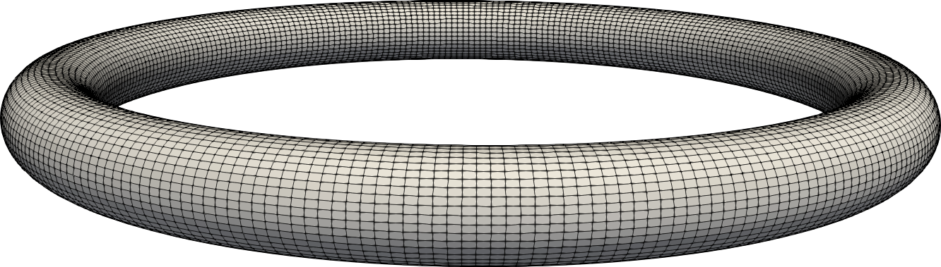
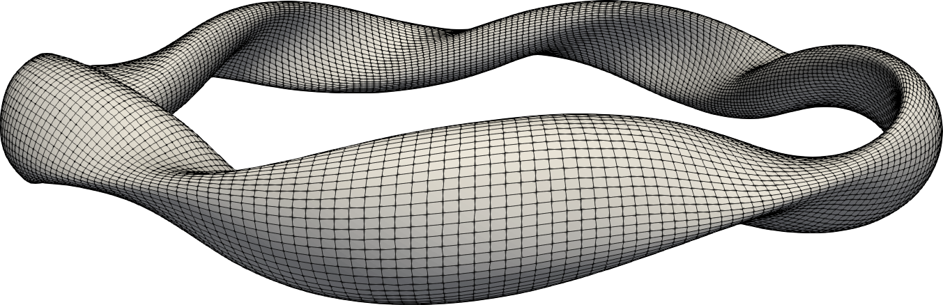
Figure 2: The surfaces used in the Green’s identity test in Section 4.1 are shown at the top. Below each surface, we plot the error $\|e\|_{\infty}$ as a function of the total number of grid points in the surface discretization. The numerical results confirm that the low-order singularity subtraction scheme of Merkel converges as $\mathcal{O}(h^{2})$ where $h=\mathcal{O}(1/\sqrt{N})$ is the mesh grid-spacing. The high-order partition of unity based scheme is expected to converge exponentially and has a numerically observed convergence rate of roughly $12$th and $10$th order respectively for the two problems.

4.2 Normal component of the magnetic field due to external coils on the W7-X plasma surface using the virtual casing principle

We now present results for computing the normal component of the external magnetic field using the numerical schemes based on Eq. 2.2 and Eq. 2.3. In the setup shown in Fig. 3, we set ${\Gamma}$ to be the surface approximating the plasma boundary in the W7-X stellarator and the magnetic field ${\mathbf{B}}$ is a Taylor state with the surface ${\Gamma}$ defined as the last closed flux surface. Taylor states are force-free magnetic fields such that $\nabla\times{\mathbf{B}}=\lambda{\mathbf{B}}$, where $\lambda$ is a known constant called the Beltrami parameter. We construct this field using the method described in [33]. The reference solution ${\mathbf{B}}_{\mathrm{ext}}\cdot{{\mathbf{n}}}$ is constructed by numerically evaluating Eq. 2.2 on a very fine mesh ($N_{u}=406$, $N_{v}=2030$) and we show convergence to this reference solution in Table 1. In both formulations, we obtain spectral convergence to nearly 10-digits.

$N_{u}~{}\times~{}N_{v}$	Error with Eq. 2.2	Error with Eq. 2.3
$14~{}\times~{}~{}~{}70$	$1.6{\text{\sc{\small e-}}}02$	$2.5{\text{\sc{\small e-}}}02$
$42~{}\times~{}~{}210$	$4.2{\text{\sc{\small e-}}}03$	$5.4{\text{\sc{\small e-}}}04$
$84~{}\times~{}~{}420$	$2.3{\text{\sc{\small e-}}}04$	$4.0{\text{\sc{\small e-}}}06$
$112~{}\times~{}~{}560$	$4.5{\text{\sc{\small e-}}}05$	$1.1{\text{\sc{\small e-}}}06$
$154~{}\times~{}~{}770$	$7.1{\text{\sc{\small e-}}}06$	$6.7{\text{\sc{\small e-}}}08$
$196~{}\times~{}~{}980$	$2.4{\text{\sc{\small e-}}}07$	$3.3{\text{\sc{\small e-}}}09$
$252~{}\times~{}1260$	$5.3{\text{\sc{\small e-}}}08$	$9.0{\text{\sc{\small e-}}}10$
$322~{}\times~{}1610$	$4.0{\text{\sc{\small e-}}}09$	$2.8{\text{\sc{\small e-}}}10$
$392~{}\times~{}1960$	$2.0{\text{\sc{\small e-}}}10$	$2.3{\text{\sc{\small e-}}}10$

Table 1: Numerical results for the experimental setup shown in Fig. 3 using the two numerical schemes described by Eq. 2.2 and Eq. 2.3. In each case, with increasing mesh resolution ($N_{u}\times N_{v}$), we report the relative error $\|{\mathbf{B}}^{0}_{ext}\cdot{{\mathbf{n}}}-{\mathbf{B}}_{ext}\cdot{{\mathbf{n}}}\|_{\infty}/\|{\mathbf{B}}\|_{\infty}$ where ${\mathbf{B}}^{0}_{ext}\cdot{{\mathbf{n}}}$ is the reference solution. The reference solution is obtained numerically using Eq. 2.2 on a very fine mesh ($N_{u}=406$, $N_{v}=2030$).

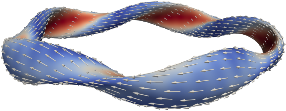
Figure 3: The plasma boundary ${\Gamma}$ in the W7-X stellarator is visualized here along with the magnetic field ${\mathbf{B}}$ for a fixed boundary calculation. The field ${\mathbf{B}}$ is a Taylor state with Beltrami parameter $\lambda=1$ and is generated using the method described in [33]. Convergence results for computing the normal component of the external field for this setup are presented in Table 1.

4.3 Vacuum field for the W7-X plasma surface and virtual casing principle

Consider the setup shown in Fig. 4, in which the internal and external currents are given by known current loops $\gamma_{1}$ and $\gamma_{2}$ respectively. The magnetic field ${\mathbf{B}}$ produced by these currents at points ${\mathbf{r}}$ on ${\Gamma}$ is given by,

$${\mathbf{B}}({\mathbf{r}})=\frac{\mu_{0}}{4\pi}\int_{\gamma_{1}}\frac{I_{1}\,\mathrm{d}{\mathbf{l}}^{\prime}\times({\mathbf{r}}-{\mathbf{r}}^{\prime})}{|{\mathbf{r}}-{\mathbf{r}}^{\prime}|^{3}}+\frac{\mu_{0}}{4\pi}\int_{\gamma_{2}}\frac{I_{2}\,\mathrm{d}{\mathbf{l}}^{\prime}\times({\mathbf{r}}-{\mathbf{r}}^{\prime})}{|{\mathbf{r}}-{\mathbf{r}}^{\prime}|^{3}},$$ (4.3)

where $I_{1}$ and $I_{2}$ are the currents in the loops $\gamma_{1}$ and $\gamma_{2}$ respectively. Since the current loops do not intersect the surface ${\Gamma}$, the integrands are smooth and these integrals can be evaluated to high precision using standard quadratures.

For our numerical test, we will now assume that we do not know the origin of the magnetic field thus calculated on the surface, and we wish to compute the normal component of the field due to the external loop $\gamma_{2}$ using the virtual casing principle. Comparing our results using the virtual casing principle with the direct calculation using the Biot-Savart law would provide a reliable test of the accuracy of our quadrature scheme. This test would be complementary to the numerical test presented in Section 4.2. However, we cannot directly apply the virtual casing principle discussed in Section 2.1 since it requires that ${\Gamma}$ be a flux surface (i.e. ${\mathbf{B}}\cdot{{\mathbf{n}}}=0$ on ${\Gamma}$). This issue can be easily circumvented by constructing a field ${\mathbf{{B}}}_{\mathrm{tot}}={\mathbf{B}}+\nabla\Phi$ in $\Omega^{\mathrm{c}}$ such that ${\mathbf{B}}_{\mathrm{tot}}\cdot{{\mathbf{n}}}=0$ on $\Gamma$. Physically, this is saying that one way of making $\Gamma$ a flux surface is to include an additional magnetic field source in $\Omega$. The corresponding potential $\Phi$ can be constructed by solving Eq. 2.7 for the unknown $\Phi$ with given boundary conditions $\nabla\Phi\cdot{{\mathbf{n}}}$. This is a Fredholm integral equation of the second kind and can therefore be solved efficiently using GMRES as described in Section 2.2. The numerical test in this section is therefore a combined test of our quadrature scheme for the two applications discussed in Section 2: the virtual casing principle and the calculation of vacuum fields. The normal component data $\nabla\Phi\cdot{{\mathbf{n}}}=-{\mathbf{B}}\cdot{{\mathbf{n}}}$ is known a priori from the construction of $\Phi$, and the tangential components of $\nabla\Phi$ are computed using Fourier differentiation of $\Phi$ on the surface. The virtual casing principle can now be be applied to ${\mathbf{{B}}}_{\mathrm{tot}}$. We use Eq. 2.2 and Eq. 2.3 to compute ${\mathbf{B}}_{\mathrm{ext}}\cdot{{\mathbf{n}}}$, where ${\mathbf{B}}_{\mathrm{ext}}$ is the field due to the external currents, namely the external current loop $\gamma_{2}$ in this example. We compare this expression with the reference normal component of the field (computed directly via Biot-Savart applied to the external current loop $\gamma_{2}$) and report convergence results in Table 2. We observe spectral convergence as we refine the mesh and reduce the tolerance $\epsilon_{\textsc{gmres}}$ for the GMRES solve. In addition, $N_{\textsc{gmres}}$ remains reasonably small since we are solving second-kind integral equations.

Finally, we observe that with a generalized version of the virtual casing principle [20], it is possible to compute all the components of the magnetic field on $\Gamma$ due to the external current loop $\gamma_{2}$ with only the magnetic field $\mathbf{B}$ on $\Gamma$ given as input. We implemented this more general numerical test as well, in which we compare all the components of ${\mathbf{B}}_{\mathrm{ext}}$, and obtained similar results to the ones reported for the normal component here. We chose to focus on the normal component in this section because it is the most common application in magnetic confinement fusion.

Figure 4: The boundary ${\Gamma}$ along with the internal ($\gamma_{1}$) and external ($\gamma_{1}$) current loops. The current loops produce a magnetic field $\mathbf{B}$ and the magnitude of this field on ${\Gamma}$ is shown. Using the methods described in Sections 2.1 and 2.2, given only the magnetic field $\mathbf{B}$ on ${\Gamma}$, we can recover the magnetic field on ${\Gamma}$ due to the external current loop $\gamma_{2}$. In Table 2, we show convergence results by comparing the external field recovered from $\mathbf{B}$ with the field computed directly from integrating over the external current loop $\gamma_{2}$.

$N_{u}~{}\times~{}N_{v}$	$\epsilon_{\textsc{gmres}}$	$N_{\textsc{gmres}}$	Error with Eq. 2.2	Error with Eq. 2.3
$14~{}\times~{}~{}~{}70$	$1{\text{\sc{\small e-}}}01$	$3$	$1.2{\text{\sc{\small e-}}}01$	$1.0{\text{\sc{\small e-}}}01$
$42~{}\times~{}~{}210$	$3{\text{\sc{\small e-}}}03$	$6$	$2.2{\text{\sc{\small e-}}}02$	$1.5{\text{\sc{\small e-}}}02$
$84~{}\times~{}~{}420$	$1{\text{\sc{\small e-}}}04$	$8$	$9.2{\text{\sc{\small e-}}}04$	$2.8{\text{\sc{\small e-}}}04$
$112~{}\times~{}~{}560$	$3{\text{\sc{\small e-}}}05$	$9$	$1.0{\text{\sc{\small e-}}}04$	$5.2{\text{\sc{\small e-}}}05$
$154~{}\times~{}~{}770$	$1{\text{\sc{\small e-}}}06$	$13$	$2.0{\text{\sc{\small e-}}}05$	$5.6{\text{\sc{\small e-}}}06$
$196~{}\times~{}~{}980$	$1{\text{\sc{\small e-}}}07$	$14$	$1.1{\text{\sc{\small e-}}}06$	$5.3{\text{\sc{\small e-}}}07$
$252~{}\times~{}1260$	$1{\text{\sc{\small e-}}}08$	$16$	$9.6{\text{\sc{\small e-}}}08$	$7.3{\text{\sc{\small e-}}}08$
$322~{}\times~{}1610$	$1{\text{\sc{\small e-}}}09$	$18$	$1.6{\text{\sc{\small e-}}}08$	$1.1{\text{\sc{\small e-}}}08$
$392~{}\times~{}1960$	$1{\text{\sc{\small e-}}}10$	$20$	$1.2{\text{\sc{\small e-}}}09$	$8.3{\text{\sc{\small e-}}}10$

Table 2: Numerical results for the experimental setup described in Section 4.3. As we refine the mesh and reduce the tolerance $\epsilon_{\textsc{gmres}}$ for the GMRES solve, we observe spectral convergence in the relative error $\|{\mathbf{B}}^{0}_{ext}\cdot{{\mathbf{n}}}-{\mathbf{B}}_{ext}\cdot{{\mathbf{n}}}\|_{\infty}/\|{\mathbf{B}}\|_{\infty}$ where ${\mathbf{B}}^{0}_{ext}\cdot{{\mathbf{n}}}$ is the reference solution computed by directly integrating along the external current loop $\gamma_{2}$. For each case, we also report the number of GMRES iterations $N_{\textsc{gmres}}$ in computing the potential $\phi$.

5 Summary

We have presented a numerical quadrature scheme for the evaluation of integrals with singular kernels appearing in magnetostatic problems for magnetic confinement fusion applications. We demonstrated that our scheme has high-order convergence, and is much more accurate than the schemes currently used in the magnetic fusion community, even for the coarsest meshes. Implementing our algorithm in current magnetic fusion codes based on integral formulations with singular kernels would significantly improve their accuracy for a fixed mesh size; conversely, for a fixed target accuracy, our scheme would allow these codes to use significantly coarser meshes. Although we have not done so for the numerical tests presented in this article, our scheme can be coupled with fast multipole methods to obtain optimal asymptotic scaling for sufficiently large-scale problems.

There are two immediate extensions to the work presented in this article. The first is the development of a fast, high-order quadrature scheme for the evaluation of integrals with singular kernels on surfaces with edges, which is needed for situations in which the surface has one or several magnetic separatrices. The second extension is the construction of a fast and high-order quadrature scheme for the evaluation of integrals with singular kernels at points away from the surface but close to it (there is no particular numerical issue for points far away from the surface). Such a scheme would, for example, be necessary if we wanted to evaluate the off-surface vacuum field potential $\Phi$ given by (2.8), or to compute the off-surface magnetic field near a bounding surface in the integral equation formulation of the calculation of Taylor states as implemented in BIEST [33]. Both extensions reflect questions which have not yet been addressed in a definitive way by the applied mathematics community [23, 21, 24, 46, 45, 26, 55, 12, 4, 5, 51, 27, 53, 1, 48, 54, 44, 9, 8]. These problems are the subject of ongoing work, with results to be reported in the future.

6 Acknowledgements

The authors would like to thank Allen Boozer for bringing to our attention the question treated in this article. D.M. was partially supported by the Office of Naval Research under award number #N00014-17-1-2451, the Simons Foundation/SFARI (560651, AB), and the U.S. Department of Energy, Office of Science, Fusion Energy Sciences under Awards No. DE-FG02-86ER53223 and DE-SC0012398. A.J.C. was partially supported by the Simons Foundation/SFARI (560651, AB), and the U.S. Department of Energy, Office of Science, Fusion Energy Sciences under Award Nos. DE-FG02-86ER53223 and DE-SC0012398. M.O. was partially supported by the Office of Naval Research under award numbers #N00014-17-1-2451 and #N00014-17-1-2059, and the Simons Foundation/SFARI (560651, AB). E.T. was partially supported by the U.S. Department of Energy, Office of Science, Fusion Energy Sciences under Award Nos. DE-FG02-86ER53223 and DE-SC0012398.

References

- [1] L. af Klinteberg and A.-K. Tornberg. Fast Ewald summation for Stokesian particle suspensions. International Journal for Numerical Methods in Fluids, 76(10):669–698, Sep 2014.
- [2] R. Albanese and G. Rubinacci. Integral formulation for 3D eddy-current computation using edge elements. IEE Proceedings A - Physical Science, Measurement and Instrumentation, Management and Education - Reviews, 135(7):457–462, Sep 1988.
- [3] C. V. Atanasiu, A. H. Boozer, L. E. Zakharov, A. A. Subbotin, and G. I. Miron. Determination of the vacuum field resulting from the perturbation of a toroidally symmetric plasma. Physics of Plasmas, 6(7):2781–2790, Jul 1999.
- [4] J. Bremer and Z. Gimbutas. A Nyström method for weakly singular integral operators on surfaces. Journal of Computational Physics, 231(14):4885–4903, May 2012.
- [5] J. Bremer and Z. Gimbutas. On the numerical evaluation of the singular integrals of scattering theory. Journal of Computational Physics, 251:327–343, Oct 2013.
- [6] O. P. Bruno and L. A. Kunyansky. A fast, high-order algorithm for the solution of surface scattering problems: Basic implementation, tests, and applications. Journal of Computational Physics, 169(1):80–110, May 2001.
- [7] O. P. Bruno and L. A. Kunyansky. Surface scattering in three dimensions: an accelerated high-order solver. Proceedings of the Royal Society of London. Series A: Mathematical, Physical and Engineering Sciences, 457(2016):2921–2934, Dec 2001.
- [8] C. Carvalho, S. Khatri, and A. D. Kim. Asymptotic approximations for the close evaluation of double-layer potentials. arXiv e-prints, page arXiv:1810.02483, Oct 2018.
- [9] C. Carvalho, S. Khatri, and A. D. Kim. Close evaluation of layer potentials in three dimensions. arXiv e-prints, page arXiv:1807.02474, Jul 2018.
- [10] M. Chance, A. Turnbull, and P. Snyder. Calculation of the vacuum Green’s function valid even for high toroidal mode numbers in tokamaks. Journal of Computational Physics, 221(1):330–348, Jan 2007.
- [11] M. S. Chance. Vacuum calculations in azimuthally symmetric geometry. Physics of Plasmas, 4(6):2161–2180, Jun 1997.
- [12] E. Corona, L. Greengard, M. Rachh, and S. Veerapaneni. An integral equation formulation for rigid bodies in Stokes flow in three dimensions. Journal of Computational Physics, 332:504–519, Mar 2017.
- [13] M. Drevlak, C. Beidler, J. Geiger, P. Helander, and Y. Turkin. Optimisation of stellarator equilibria with ROSE. Nuclear Fusion, 59(1):016010, Nov 2018.
- [14] M. Drevlak, D. Monticello, and A. Reiman. Pies free boundary stellarator equilibria with improved initial conditions. Nuclear fusion, 45(7):731, 2005.
- [15] J. P. Freidberg and W. Grossmann. Magnetohydrodynamic stability of a sharp boundary model of tokamak. The Physics of Fluids, 18(11):1494–1506, 1975.
- [16] J. P. Freidberg, W. Grossmann, and F. A. Haas. Stability of a high-, l=3 stellarator. The Physics of Fluids, 19(10):1599–1607, 1976.
- [17] R. Gruber, S. Semenzato, F. Troyon, T. Tsunematsu, W. Kerner, P. Merkel, and W. Schneider. Hera and other extensions of Erato. Computer Physics Communications, 24(3):363–376, Dec 1981.
- [18] R. Gruber, F. Troyon, D. Berger, L. Bernard, S. Rousset, R. Schreiber, W. Kerner, W. Schneider, and K. Roberts. Erato stability code. Computer Physics Communications, 21(3):323–371, Jan 1981.
- [19] R. B. Guenther and J. W. Lee. Partial Differential Equations of Mathematical Physics and Integral Equations. New York: Dover Publications, Inc., 1995.
- [20] J. D. Hanson. The virtual-casing principle and Helmholtz’s theorem. Plasma Physics and Controlled Fusion, 57(11):115006, Sep 2015.
- [21] J. Helsing. A fast and stable solver for singular integral equations on piecewise smooth curves. SIAM Journal on Scientific Computing, 33(1):153–174, Jan 2011.
- [22] J. Helsing and A. Karlsson. An explicit kernel-split panel-based Nyström scheme for integral equations on axially symmetric surfaces. Journal of Computational Physics, 272:686–703, Sep 2014.
- [23] J. Helsing and R. Ojala. Corner singularities for elliptic problems: Integral equations, graded meshes, quadrature, and compressed inverse preconditioning. Journal of Computational Physics, 227(20):8820–8840, Oct 2008.
- [24] J. Helsing and K.-M. Perfekt. On the polarizability and capacitance of the cube. Applied and Computational Harmonic Analysis, 34(3):445–468, May 2013.
- [25] S. Hirshman, W. van RIJ, and P. Merkel. Three-dimensional free boundary calculations using a spectral Green’s function method. Computer Physics Communications, 43(1):143–155, Dec 1986.
- [26] J. G. Hoskins, V. Rokhlin, and K. Serkh. On the numerical solution of elliptic partial differential equations on polygonal domains. SIAM Journal on Scientific Computing, 41(4):A2552–A2578, Jan 2019.
- [27] A. Klöckner, A. Barnett, L. Greengard, and M. O’Neil. Quadrature by expansion: A new method for the evaluation of layer potentials. Journal of Computational Physics, 252:332–349, Nov 2013.
- [28] K. Lackner. Computation of ideal MHD equilibria. Computer Physics Communications, 12(1):33–44, Sep 1976.
- [29] M. Landreman. An improved current potential method for fast computation of stellarator coil shapes. Nuclear Fusion, 57(4):046003, Feb 2017.
- [30] D. Lazanja. Components of the magnetic field from interior and exterior sources in toroidal geometry. PhD thesis, Columbia University, 2011.
- [31] S. A. Lazerson. The virtual-casing principle for 3d toroidal systems. Plasma Physics and Controlled Fusion, 54(12):122002, 2012.
- [32] J. P. Lee, A. Cerfon, J. P. Freidberg, and M. Greenwald. Tokamak elongation - how much is too much? part 2. numerical results. Journal of Plasma Physics, 81(6):515810608, Dec 2015.
- [33] D. Malhotra, A. Cerfon, L.-M. Imbert-Gérard, and M. O’Neil. Taylor states in stellarators: A fast high-order boundary integral solver. Journal of Computational Physics, 397:108791, Nov 2019.
- [34] A. Marx and H. Lütjens. Free-boundary simulations with the XTOR-2f code. Plasma Physics and Controlled Fusion, 59(6):064009, May 2017.
- [35] P. Merkel. A Green’s function method for the vacuum contribution to the MHD stability of helically symmetric equilibria. Zeitschrift fur Naturforschung - Section A Journal of Physical Sciences, 37(8):859–865, Aug 1982.
- [36] P. Merkel. An integral equation technique for the exterior and interior Neumann problem in toroidal regions. Journal of Computational Physics, 66(1):83–98, Sep 1986.
- [37] P. Merkel. Solution of stellarator boundary value problems with external currents. Nuclear Fusion, 27(5):867–871, May 1987.
- [38] A. I. Morozov and L. S. Solov’ev. Motion of Charged Particles in Electromagnetic Fields. Reviews of Plasma Physics, 2:201, Jan 1966.
- [39] M. O’Neil and A. J. Cerfon. An integral equation-based numerical solver for Taylor states in toroidal geometries. Journal of Computational Physics, 359:263–282, Apr 2018.
- [40] V. Pustovitov. Magnetic diagnostics: General principles and the problem of reconstruction of plasma current and pressure profiles in toroidal systems. Nuclear fusion, 41(6):721, 2001.
- [41] V. Pustovitov. Decoupling in the problem of tokamak plasma response to asymmetric magnetic perturbations. Plasma Physics and Controlled Fusion, 50(10):105001, 2008.
- [42] V. D. Pustovitov. General formulation of the resistive wall mode coupling equations. Physics of Plasmas, 15(7):072501, Jul 2008.
- [43] M. Rachh, A. Klöckner, and M. O ’Neil. Fast algorithms for Quadrature by Expansion I: Globally valid expansions. Journal of Computational Physics, 345:706–731, Sep 2017.
- [44] A. Rahimian, A. Barnett, and D. Zorin. Ubiquitous evaluation of layer potentials using Quadrature by Kernel-Independent Expansion. BIT Numerical Mathematics, 58(2):423–456, Nov 2017.
- [45] K. Serkh. On the solution of elliptic partial differential equations on regions with corners II: Detailed analysis. Applied and Computational Harmonic Analysis, 46(2):250–287, Mar 2019.
- [46] K. Serkh and V. Rokhlin. On the solution of elliptic partial differential equations on regions with corners. Journal of Computational Physics, 305:150–171, Jan 2016.
- [47] V. Shafranov and L. Zakharov. Use of the virtual-casing principle in calculating the containing magnetic field in toroidal plasma systems. Nuclear Fusion, 12(5):599–601, Sep 1972.
- [48] M. Siegel and A.-K. Tornberg. A local target specific quadrature by expansion method for evaluation of layer potentials in 3D. Journal of Computational Physics, 364:365–392, Jul 2018.
- [49] J. A. Stratton. Electromagnetic theory, mcgrow-hill book company. Inc., New York, and London, 1941.
- [50] E. Strumberger. Finite- magnetic field line tracing for Helias configurations. Nuclear Fusion, 37(1):19–27, Jan 1997.
- [51] S. Tlupova and J. T. Beale. Nearly singular integrals in 3D Stokes flow. Communications in Computational Physics, 14(5):1207–1227, Nov 2013.
- [52] L. N. Trefethen and J. A. C. Weideman. The exponentially convergent trapezoidal rule. SIAM Review, 56(3):385–458, Jan 2014.
- [53] M. Wala and A. Klöckner. A fast algorithm for Quadrature by Expansion in three dimensions. Journal of Computational Physics, 388:655–689, Jul 2019.
- [54] L. Ying, G. Biros, and D. Zorin. A high-order 3D boundary integral equation solver for elliptic pdes in smooth domains. Journal of Computational Physics, 219(1):247–275, Nov 2006.
- [55] H. Zhao, A. H. Isfahani, L. N. Olson, and J. B. Freund. A spectral boundary integral method for flowing blood cells. Journal of Computational Physics, 229(10):3726–3744, May 2010.