Charged lepton flavour change and Non-Standard neutrino Interactions

Abstract

Non-Standard neutrino Interactions (NSI) are vector contact interactions involving two neutrinos and two first generation fermions, which can affect neutrino propagation in matter. SU(2) gauge invariance suggests that NSI should be accompanied by more observable charged lepton contact interactions. However, these can be avoided at tree level in various ways. We focus on lepton flavour-changing NSI, suppose they are generated by New Physics heavier than $m_{W}$ that does not induce (charged) Lepton Flavour Violation (LFV) at tree level, and show that LFV is generated at one loop in most cases. The current constraints on charged Lepton Flavour Violation therefore suggest that $\mu\leftrightarrow e$ flavour-changing NSI are unobservable and $\tau\leftrightarrow\ell$ flavour-changing NSI are an order of magnitude weaker than the weak interactions. This conclusion can be avoided if the heavy New Physics conspires to cancel the one-loop LFV, or if NSI are generated by light New Physics to which our analysis does not apply.

I Introduction and review

Non-Standard neutrino Interactions (NSI) are four-fermion interactions induced by physics from Beyond-the-Standard Model, constructed from a vector current of two Standard Model (SM) neutrinos of flavour $\rho$ and $\sigma$, and two first generation fermions $f\in\{e,u,d\}$. Below the weak scale, such interactions can be included in the Lagrangian as

$$-2\sqrt{2}G_{F}\varepsilon_{f}^{\rho\sigma}(\overline{\nu}_{\rho}\gamma_{\alpha}P_{L}\nu_{\sigma})(\overline{f}\gamma^{\alpha}P_{X}f)$$ (I.1)

where $G_{F}=1/(2\sqrt{2}v^{2})$ is the Fermi constant, the dimensionless coefficient $\varepsilon^{\rho\sigma}$ parametrises the strength of these new interactions, $P_{X}$ is a chiral projector $P_{L/R}=(1\pm\gamma_{5})/2$, and $f$ will be referred to as the “external” fermion.

NSI were introduced NSI1 as “New Physics” that can be searched for in neutrino oscillations. Indeed, in matter, the first generation fermion current can be replaced by the fermion number density in the medium: $(\overline{f}\gamma^{\alpha}P_{X}f)\to\delta^{\alpha 0}n_{f}/2$. At finite density, NSI therefore contribute an effective mass to the oscillation Hamiltonian of neutrinos:

$$\frac{[\Delta m^{2}]^{\rho\sigma}}{E}\sim\sqrt{2}G_{F}\varepsilon_{f}^{\rho\sigma}n_{f}~{}~{}~{}.$$

Charged current NSI, involving a $\nu$, a charged lepton and differently charged external fermions, are also studied because they affect the production and detection of neutrinos. However, they are not considered in this manuscript, where “NSI” is taken to mean neutral current NSI.

The phenomenology of NSI has been widely studied (for a review, see eg revFT ), because they can contribute in neutral current neutrino scattering BR ; DP-GRS ; Biggio:2009nt , and via the matter effect to neutrino oscillations in Long Baseline experiments LBNL , the sun and the atmosphere atm ; GGetal18 , supernovae SN1 , neutron stars NS , and the early Universe deSalasSergio ; Serpico . In particular, the effects of NSI in terrestrial neutrino oscillation experiments have been carefully studied, in order to explore the prospects of disentangling NSI from the minimal set of mixing angles, masses and phases confusion ; LBNL .

More recently, “Generalised Neutrino Interactions”(GNI) have been discussed ASdRR ; ATZ ; FGAX ; Bischer:2019ttk , which involve two light neutrinos, and two first generation fermions. Since the neutrinos are only required to be light, but not members of an SM doublet, GNI include scalar and tensor four-fermion operators involving sterile “right-handed” neutrinos:

$$(\overline{\nu_{R}}_{\rho}\nu_{L\sigma})(\overline{f}P_{X}f)~{}~{},~{}~{}~{}(\overline{\nu_{R}}_{\rho}\sigma^{\alpha\beta}\nu_{L\sigma})(\overline{f}\sigma_{\alpha\beta}P_{L}f)~{}~{}~{},$$

where $\sigma^{\alpha\beta}=\frac{i}{2}[\gamma^{\alpha},\gamma^{b}]$. Such scalar (and tensor) interactions are interesting, because the COHERENT experiment COHERENT measured neutrino scattering on nuclei at momentum transfer $\sim 30-70$ MeV, where the cross-section is coherently enhanced $\propto A^{2}$ (where $A=$ atomic number). Unlike the “matter effect”, which is a forward scattering amplitude so only a vector current of SM neutrinos can contribute, the COHERENT cross-section is sensitive to the scalar interaction (which is coherently enhanced), as well as having reduced sensitivity to the tensor interaction. In this manuscript, we focus on NSI.

The bounds on NSI from neutrino scattering experiments BR ; DP-GRS , are of order $|\varepsilon_{f}^{\rho\sigma}|\mathrel{\vbox{\hbox{$<$}\nointerlineskip\hbox{$\sim$}}}0.1\to 1$. A recent combined fit GGetal18 to current oscillation data and the results of the COHERENT experiment gives bounds $|\varepsilon_{f}^{\rho\sigma}|\mathrel{\vbox{\hbox{$<$}\nointerlineskip\hbox{$\sim$}}}0.01$, except on the diagonal, where NSI large enough to flip the sign of the SM contribution are allowed. The authors of this study assume that the flavour structure of NSI on $e$s, $u$s or $d$s is the same (so $\varepsilon_{f}^{\rho\sigma}=\varepsilon_{f}\varepsilon^{\rho\sigma}$), and that NSI are a small perturbation around the standard parameters that give best fit solutions in the absence of NSI. With these assumptions, they set constraints on NSI, meaning that larger values are excluded. The results of the COHERENT experiment are an important input to this analysis, because the oscillation data is sensitive to differences in the eigenvalues of the propagation Hamiltonian, whereas the COHERENT results constrain the neutral current scattering rate. So large flavour-diagonal NSI are constrained by COHERENT. The COHERENT constraints alone, without assumptions about the flavour structure of $\varepsilon$, are discussed in Giunti:2019xpr .

In the Standard Model, neutrinos share an SU(2) doublet with charged leptons, so that SM gauge-invariant operators that mediate NSI may also mediate stringently constrained, charged lepton flavour changing processes. For instance, the contact interaction of eqn (I.1), for $f=e_{L}$, could be generated by the dimension six operator

$$-2\sqrt{2}G_{F}\varepsilon_{e}^{\rho\sigma}(\overline{\ell}_{\rho}\gamma^{\alpha}\ell_{\sigma})(\overline{\ell}_{e}\gamma_{\alpha}\ell_{e})$$ (I.2)

where $\bar{\ell}$ is the SU(2) doublet $(\overline{\nu_{L}},\overline{e_{L}})$. However, this operator also induces the four-charged-lepton interaction $(\overline{e}_{\rho}\gamma^{\alpha}P_{L}e_{\sigma})(\overline{e}\gamma_{\alpha}P_{L}e)$ whose coefficient would be strictly constrained by decays $e_{\sigma}\to e_{\rho}e\bar{e}$. These concerns can be avoided by instead constructing NSI at dimension eight in the SMEFT, for instance as

$$-2\sqrt{2}G_{F}\varepsilon_{f}^{\rho\sigma}(\overline{\nu}_{\rho}\gamma_{\alpha}\nu_{\sigma})(\overline{f}\gamma^{\alpha}f)~{}~{}\longleftarrow~{}~{}\frac{C_{f}^{\rho\sigma}}{\Lambda_{NP}^{4}}(\overline{\ell}^{p}_{\rho}\epsilon_{pQ}H^{Q*})\gamma_{\alpha}(H^{R}\epsilon_{Rs}\ell^{s}_{\sigma})(\overline{f}\gamma^{\alpha}f)$$ (I.3)

where $\epsilon_{pQ}$ is the antisymmetric SU(2) contraction given in eqn (A.9). When the Higgs $H=(H^{+},H_{0})$ takes a vacuum expectation value $\langle H_{0}\rangle=v$, the dimension eight operator reproduces the contact interaction on the left (this is discussed in more detail in section II), with

$$\varepsilon_{f}^{\rho\sigma}=C_{f}^{\rho\sigma}\frac{v^{4}}{\Lambda_{NP}^{4}}~{}~{}.$$ (I.4)

It is clear that to obtain $\varepsilon\mathrel{\vbox{\hbox{$>$}\nointerlineskip\hbox{$\sim$}}}10^{-3}$, the New Physics scale $\Lambda_{NP}$ cannot be far above the weak scale and is likely to be within the reach of the LHC.

Models that generate such large effects in the neutrino sector, while avoiding the stringent bounds on charged Lepton Flavour Violation(LFV) PSI , have been explored by various authors. The authors of GXOW considered the case where NSI were generated at tree level by the exchange of new particles of mass $\mathrel{\vbox{\hbox{$>$}\nointerlineskip\hbox{$\sim$}}}m_{W}$, and required that the heavy mediators not induce tree-level LFV interactions at dimension six or eight. They allowed for cancellations among the mediators of operators of a given dimension, but not for cancellations between the coefficients of operators of different dimension, and found various viable models. Similarly, reference Antusch considered models with heavy new particles that induced NSI at tree level, however these authors did not allow cancellations among the contributions of different mediators to LFV interactions. They showed that their allowed models induced additional, better constrained operators, so that $\varepsilon\mathrel{\vbox{\hbox{$>$}\nointerlineskip\hbox{$\sim$}}}10^{-2}$ was excluded. In this manuscript, we review this question from an EFT perspective allowing arbitrary cancellations, also between operators of dimension six and eight, in order to find linear combinations of operators that induce NSI but not LFV at tree level.

Models with light mediators have also been constructed PP ; FarzanModel ; FarzanModel2 . Such models are motivated, because a detectable $\varepsilon$ cannot be small, suggesting that any heavy mediator could be within the range of the LHC. The models of PP ; FarzanModel involve a light ($\mathrel{\vbox{\hbox{$>$}\nointerlineskip\hbox{$\sim$}}}10$ MeV) feebly coupled $Z^{\prime}$, which can avoid tree-level LFV constraints by a suitable choice of couplings; in FarzanModel2 , the SM neutrinos share mass terms with additional singlets, which are charged under the U’(1).

Even if the New Physics responsible for NSI does not induce LFV at tree level, loop effects could mix NSI and LFV operators. Reference DP-GRS considered a particular dimension eight NSI operator, and erroneously argued that the exchange of a $W$ boson between the two neutrino legs would transform them into charged leptons, thereby inducing a contact interaction that was severely constrained by experimental bounds on charged Lepton Flavour Violation (LFV). However, it was pointed out in Biggio , that the log-enhanced, one-loop mixing of this NSI operator into LFV operators vanished. The apparent conclusion was that at one loop, there is no model-independent constraint on NSI from LFV.

In this manuscript, we revisit the EFT description of NSI, and the LFV it induces via electroweak loops. We are therefore neglecting models with light mediators, and our results apply when NSI are present as a contact interaction above the weak scale, where the usual SMEFT can be applied. In section II, we introduce the two sets of operators that we will use in the analysis: SU(2)-invariant operators for the EFT above the weak scale, and QED$\times$QCD invariant operators below $m_{W}$. Also, the matching between the bases is given and the operator combinations that induce either NSI, or LFV, at low energy are listed. Section III is about Renormalisation Group Equations (RGEs), which encode the Higgs and $W$ loops that mix NSI and LFV at scales above $m_{W}$. In this manuscript, we limit ourselves to one-loop RGEs, which describe the logⁿ-enhanced part of all $n$-loop diagrams. The one-loop RGEs are known for dimension six operators JMT , and those for our dimension eight operators are obtained in section III. Finally, in the results section IV, which should be accessible without reading the more technical section III, we show that in most cases, the operator combinations that at tree level match onto NSI without LFV, induce LFV at one loop via the RGEs. The resulting sensitivities of LFV processes to NSI are given. We summarise in section V.

II Operators

II.1 In the $SU(3)\times SU(2)\times U(1)$ theory above $m_{W}$

We suppose a New Physics model at a scale $\Lambda_{NP}>m_{W}$, that induces lepton-flavour-changing vector operators of dimension six and eight, which at tree level generate (neutral current) NSI but no LFV. We want to know whether Higgs or $W$ loops could mix such operators into LFV operators, so we need a list of NSI/LFV vector operators of dimension eight and six. These operators will be added to the SM Lagrangian as ${\cal L}_{SM}\to{\cal L}_{SM}+\delta{\cal L}$, with

$$\delta{\cal L} = \sum_{O,\zeta}\frac{C_{O}^{\zeta}}{\Lambda_{NP}^{2n}}{\cal O}_{O}^{\zeta}+h.c.$$ (II.1)

where $n=1$ or 2 for respectively dimension six or eight operators, $\{O\}$ is the basis of operators with Lorentz structure $\gamma_{\alpha}\otimes\gamma^{\alpha}$, and $\zeta$ represents the flavour indices $\rho\sigma ff$. To avoid cluttering the notation, the flavour indices are sometimes reduced to $\rho\sigma$ or suppressed. Greek indices from the beginning of the alphabet ($\alpha,\beta$…) are Lorentz indices, and those from the end of the alphabet ($\sigma,\rho$…) are charged lepton flavour indices. The New Physics scale $\Lambda_{NP}$ is required to be above $m_{W}$, but is otherwise undetermined, being one of the parameters controlling the size of $\varepsilon_{f}^{\rho\sigma}$ (see eqn I.4). In later sections, loop effects containing $\ln(\Lambda_{NP}/m_{W})$ will arise, which we conservatively take $\simeq 1$.

The Higgs doublet is written

$${H}=\left(\begin{array}[]{c}H^{+}\\ H_{0}\end{array}\right)\to\left(\begin{array}[]{c}0\\ v\end{array}\right)$$ (II.2)

where after the arrow is the vacuum expectation value with $1/v^{2}=2\sqrt{2}G_{F}$, and the Higgs is included in the Standard Model Lagrangian (in the mass eigenstates of charged leptons) as

$${\cal L}_{SM} = \overline{\ell}i\,D\!\!\!\!/~{}\ell+...-\{y^{\rho}_{e}\overline{\ell}_{\rho}He^{\rho}_{R}+h.c.\}+(D_{\mu}H)^{\dagger}D^{\mu}H-M^{2}H^{\dagger}H+\frac{\lambda}{2}(H^{\dagger}H)^{2}~{}~{}~{}.$$ (II.3)

where the physical Higgs mass $\simeq 125$ GeV is $m^{2}_{h}=\lambda v^{2}$, which corresponds to $\lambda\simeq 1/2$. At tree level, the minimum of the Higgs potential is given by

$$M^{2}-\lambda v^{2}=0~{}~{},$$ (II.4)

and the one-loop minimisation is discussed in Appendix C. Since we will write RGEs for operators of dimension six and eight, which can mix due to Higgs mass insertions, we will frequently use a parameter

$$\eta\equiv\frac{M^{2}}{\Lambda_{NP}^{2}}~{}~{},~{}~{}\frac{\eta}{\lambda}=\frac{v^{2}}{\Lambda_{NP}^{2}}~{}.$$ (II.5)

Consider first to construct operators involving doublet leptons and SU(2) singlet external fermions $f$. The dimension six vector operator of the “Warsaw” basis polonais is

$${\cal O}^{\rho\sigma}_{M2,f}\equiv(\overline{\ell}_{\rho}\gamma_{\alpha}\ell_{\sigma})(\overline{f}\gamma^{\alpha}f)~{}~{}~{},$$ (II.6)

referred to as “M2”, because the dimension eight operators will mix into it via insertions of the Higgs mass parameter $M^{2}$. At dimension eight, a convenient basis is

$${\cal O}^{\rho\sigma}_{NSI,f}\equiv(\overline{\ell}_{\rho}\epsilon H^{*})\gamma_{\alpha}(H\epsilon\ell_{\sigma})(\overline{f}\gamma^{\alpha}f)~{}~{}~{},~{}~{}~{}{\cal O}^{\rho\sigma}_{H2,f}\equiv(\overline{\ell}_{\rho}H\gamma_{\alpha}H^{\dagger}\ell_{\sigma})(\overline{f}\gamma^{\alpha}f)~{}~{}~{},$$ (II.7)

where $\epsilon$ is the totally anti-symmetric tensor in two dimensions. There could be additional operators with derivatives, but we neglect the Yukawa couplings, in which limit the derivative operators vanish by the equations of motion.

For the case where the external fermions are SU(2) doublets, the Warsaw basis (of dimension six operators) contains ${\cal O}_{M2,f}$ for $f\in\{\ell,q\}$, and also the triplet contraction $(\overline{\ell}_{\rho}\vec{\tau}\gamma_{\alpha}\ell_{\sigma})(\overline{q}\vec{\tau}\gamma^{\alpha}q)$. The analogous four-lepton triplet contraction is not included, because it can be rewritten:

$$(\overline{\ell}_{\mu}\vec{\tau}\gamma_{\alpha}\ell_{\tau})(\overline{\ell}_{e}\vec{\tau}\gamma^{\alpha}\ell_{e})=2(\overline{\ell}_{\mu}\gamma_{\alpha}\ell_{e})(\overline{\ell}_{e}\gamma^{\alpha}\ell_{\tau})-(\overline{\ell}_{\mu}\gamma_{\alpha}\ell_{\tau})(\overline{\ell}_{e}\gamma^{\alpha}\ell_{e})~{}~{}.$$

The singlet operators are more convenient for matching to low-energy four-fermion operators than the triplets, so we make a similar transformation for the triplet operator involving quarks, and take at dimension six for external doublet quarks:

$${\cal O}^{\rho\sigma}_{M2,q}\equiv(\overline{\ell}_{\rho}\gamma_{\alpha}\ell_{\sigma})(\overline{q}\gamma^{\alpha}q)~{}~{}~{},~{}~{}{\cal O}^{\rho\sigma}_{LQM2,q}\equiv(\overline{\ell}_{\rho}\gamma_{\alpha}q)(\overline{q}\gamma^{\alpha}\ell_{\sigma})~{}~{}~{}.$$ (II.8)

At dimension eight, Rossi and Berezhiani BR propose five operators

$${\cal O}^{\rho\sigma}_{S}=(\overline{\ell}_{\rho}\gamma_{\alpha}\ell_{\sigma})(\overline{q}\gamma^{\alpha}q)(H^{\dagger}H) {\cal O}_{TLH}^{\rho\sigma}=(\overline{\ell}_{\rho}\tau^{a}\gamma_{\alpha}\ell_{\sigma})(\overline{q}\gamma^{\alpha}q)(H^{\dagger}\tau^{a}H)$$

$${\cal O}_{TQH}^{\rho\sigma}=(\overline{\ell}_{\rho}\gamma_{\alpha}\ell_{\sigma})(\overline{q}\gamma^{\alpha}\tau^{a}q)(H^{\dagger}\tau^{a}H) {\cal O}_{TLQ}^{\rho\sigma}=(\overline{\ell}_{\rho}\tau^{a}\gamma_{\alpha}\ell_{\sigma})(\overline{q}\tau^{a}\gamma^{\alpha}q)(H^{\dagger}H)$$

$$(\overline{\ell}_{\rho}\tau^{a}\gamma_{\alpha}\ell_{\sigma})(\overline{q}\tau^{b}\gamma^{\alpha}q)(H^{\dagger}\tau^{c}H)\epsilon_{abc} \equiv {\cal O}^{\rho\sigma}_{TTT}$$ (II.9)

where to be concrete, the external fermion is taken to be a first generation quark doublet. The first two operators would be present for singlet external currents.

In order to count the number of operators, notice that it corresponds to the number of independent SU(2) contractions for an operator constructed from the fields:

$$(\overline{\ell}^{i}_{\rho}\gamma_{\alpha}\ell^{j}_{\sigma})(\overline{q}^{k}\gamma^{\alpha}q^{l})(H^{\dagger M}H^{N})$$

where $\{i,j,k,l,M,N\}$ are SU(2) indices. The possible contractions involve three $\tau$s, one $\delta$ and two $\tau$s, one $\delta$ and two $\epsilon$s, or three $\delta$s. But the $\tau\tau\tau$, $\delta\tau\tau$ and $\delta\epsilon\epsilon$ contractions can be rewritten as three $\delta$s using the Fierz or SU(2) identities given in eqn (A.10). Then there are six $\delta\delta\delta$ contractions, among which we find one relation, leaving five independent operators (This is discussed in more detail in Appendix B).

It is convenient to use an alternative basis without triplet contractions ${\cal O}^{\rho\sigma}_{TTT}$, to simplify the matching onto the Higgsless theory below $m_{W}$. The dimension six operators in our basis, in the case where the external fermion is the first generation quark doublet $q$, are

$${\cal O}^{\rho\sigma}_{M2,q}\equiv(\overline{\ell}_{\rho}\gamma_{\alpha}\ell_{\sigma})(\overline{q}\gamma_{\alpha}q)~{}~{}~{} ~{}~{}~{}{\cal O}^{\rho\sigma}_{LQM2,q}\equiv(\overline{\ell}_{\rho}\gamma_{\alpha}q)(\overline{q}\gamma_{\alpha}\ell_{\sigma})$$ , (II.10)

where the SU(2) contractions are inside parentheses. At dimension eight, we take

$${\cal O}^{\rho\sigma}_{NSI,q}\equiv(\overline{\ell}_{\rho}\epsilon H^{*})\gamma_{\alpha}(H\epsilon\ell_{\sigma})(\overline{q}\gamma^{\alpha}q)~{}~{}~{} ~{}~{}~{}{\cal O}^{\rho\sigma}_{H2,q}\equiv(\overline{\ell}_{\rho}H)\gamma_{\alpha}(H^{\dagger}\ell_{\sigma})(\overline{q}\gamma^{\alpha}q)$$ ,

$${\cal O}^{\rho\sigma}_{CCLFV,q}\equiv(\overline{\ell}_{\rho}\gamma_{\alpha}q)(\overline{q}H)\gamma_{\alpha}(H^{\dagger}\ell_{\sigma})~{}~{}~{} ~{}~{}~{}[{\cal O}^{\dagger}_{CCLFV,q}]^{\rho\sigma}\equiv(\overline{\ell}_{\rho}H)\gamma_{\alpha}(H^{\dagger}q)(\overline{q}\gamma_{\alpha}\ell_{\sigma})$$ , (II.11)

$${\cal O}^{\rho\sigma}_{CCNSI+,q}\equiv({\cal O}^{\rho\sigma}_{CCNSI,q}+[{\cal O}^{\dagger}_{CCNSI,q}]^{\rho\sigma}) \equiv (\overline{\ell}_{\rho}\gamma_{\alpha}q)(\overline{q}\epsilon H^{*})\gamma_{\alpha}(H\epsilon\ell_{\sigma})+(\overline{\ell}_{\rho}\epsilon H^{*})\gamma_{\alpha}(H\epsilon q)(\overline{q}\gamma_{\alpha}\ell_{\sigma})$$

where the SU(2) contractions are inside the parentheses. The relation of this basis to the Berezhiani-Rossi basis is discussed in appendix B.

The operators ${\cal O}_{H2}$ and ${\cal O}_{NSI}$ are hermitian(as matrices in lepton flavour space), as is the combination ${\cal O}_{CCNSI}+{\cal O}_{CCNSI}^{\dagger}$ (which corresponds to one of the $\delta\delta\delta$ contractions discussed above). The remaining two operators, ${\cal O}_{CCLFV}$ and ${\cal O}_{CCLFV}^{\dagger}$, are not hermitian, but appear in the one-loop RGEs in the combination ${\cal O}_{CCLFV,+}\equiv{\cal O}_{CCLFV}+{\cal O}_{CCLFV}^{\dagger}$. As a result, our basis of dimension eight operators for external doublets contains only four operators that mix with each other. An additional operator, ${\cal O}_{CCLFV}-{\cal O}_{CCLFV}^{\dagger}$, decouples from the operator mixing but is included in our basis for completeness. The matching of these operators onto low energy operators is given in table 1.

name		operator	below $m_{W}$
${\cal O}^{\rho\sigma}_{NSI,q}$	x	$(\overline{\ell}_{\rho}\epsilon H^{*})\gamma_{\alpha}(H\epsilon\ell_{\sigma})(\overline{q}\gamma^{\alpha}q)$	$-v^{2}(\overline{\nu}_{\rho}\gamma_{\alpha}P_{L}\nu_{\sigma})(\overline{q}\gamma^{\alpha}q)$
${\cal O}^{\rho\sigma}_{H2,q}$	x	$(\overline{\ell}_{\rho}H)\gamma_{\alpha}(H^{\dagger}\ell_{\sigma})(\overline{q}\gamma^{\alpha}q)$	$v^{2}(\overline{e}_{\rho}\gamma_{\alpha}P_{L}e_{\sigma})(\overline{q}\gamma^{\alpha}q)$
${\cal O}^{\rho\sigma}_{M2,q}$	x	$(\overline{\ell}_{\rho}\gamma_{\alpha}\ell_{\sigma})(\overline{q}\gamma^{\alpha}q)$	$(\overline{e}_{\rho}\gamma_{\alpha}P_{L}e_{\sigma}+\overline{\nu}_{\rho}\gamma_{\alpha}\nu_{\sigma})(\overline{q}\gamma^{\alpha}q)$
${\cal O}^{\rho\sigma}_{LQM2,q}$		$(\overline{\ell}_{\rho}\gamma_{\alpha}q)(\overline{q}\gamma^{\alpha}\ell_{\sigma})$	$(\overline{\nu}_{\rho}\gamma^{\alpha}P_{L}\nu_{\sigma})(\overline{u}\gamma_{\alpha}P_{L}u)+(\overline{e}_{\rho}\gamma^{\alpha}P_{L}e_{\sigma})(\overline{d}\gamma_{\alpha}P_{L}d)$
			$+(\overline{\nu}_{\rho}\gamma^{\alpha}P_{L}e_{\sigma})(\overline{d}\gamma_{\alpha}P_{L}u)+(\overline{e}_{\rho}\gamma^{\alpha}P_{L}\nu_{\sigma})(\overline{u}\gamma_{\alpha}P_{L}d)$
${\cal O}^{\rho\sigma}_{CCLFV,q}$		$(\overline{q}H)\gamma_{\alpha}(H^{\dagger}\ell_{\sigma})(\overline{\ell}_{\rho}\gamma^{\alpha}q)$	$2v^{2}(\overline{e}_{\rho}\gamma_{\alpha}P_{L}e_{\sigma})(\overline{d}\gamma^{\alpha}P_{L}d)$
$~{}+[{\cal O}^{\dagger}_{CCLFV,q}]^{\rho\sigma}$		$~{}+(\overline{\ell}_{\rho}H)\gamma_{\alpha}(H^{\dagger}q)(\overline{q}\gamma^{\alpha}\ell_{\sigma})$	$+v^{2}(\overline{e}_{\rho}\gamma_{\alpha}P_{L}\nu_{\sigma})(\overline{u}\gamma^{\alpha}P_{L}d)+v^{2}(\overline{\nu}_{\rho}\gamma_{\alpha}P_{L}e_{\sigma})(\overline{d}\gamma^{\alpha}P_{L}u)$
${\cal O}^{\rho\sigma}_{CCNSI,q}$	x	$(\overline{q}\epsilon H^{*})\gamma_{\alpha}(H\epsilon\ell_{\sigma})(\overline{\ell}_{\rho}\gamma^{\alpha}q)$	$-2v^{2}(\overline{\nu}_{\rho}\gamma_{\alpha}P_{L}\nu_{\sigma})(\overline{u}\gamma^{\alpha}P_{L}u)$
$~{}+[{\cal O}^{\dagger}_{CCNSI,q}]^{\rho\sigma}$		$~{}+(\overline{\ell}_{\rho}\epsilon H^{*})\gamma_{\alpha}(H\epsilon q)(\overline{q}\gamma^{\alpha}\ell_{\sigma})$	$-v^{2}(\overline{e}_{\rho}\gamma_{\alpha}P_{L}\nu_{\sigma})(\overline{u}\gamma^{\alpha}P_{L}d)-v^{2}(\overline{\nu}_{\rho}\gamma_{\alpha}P_{L}e_{\sigma})(\overline{d}\gamma^{\alpha}P_{L}u)$
${\cal O}^{\rho\sigma}_{CCLFV,q}$		$(\overline{q}H)\gamma_{\alpha}(H^{\dagger}\ell_{\sigma})(\overline{\ell}_{\rho}\gamma^{\alpha}q)$	$v^{2}(\overline{\nu}_{\rho}\gamma_{\alpha}P_{L}e_{\sigma})(\overline{d}\gamma^{\alpha}P_{L}u)$
$~{}-[{\cal O}^{\dagger}_{CCLFV,q}]^{\rho\sigma}$		$~{}-(\overline{\ell}_{\rho}H)\gamma_{\alpha}(H^{\dagger}q)(\overline{q}\gamma^{\alpha}\ell_{\sigma})$	$-v^{2}(\overline{e}_{\rho}\gamma_{\alpha}P_{L}\nu_{\sigma})(\overline{u}\gamma^{\alpha}P_{L}d)\par$

Table 1: SMEFT operators used in the RGEs of this paper, and four-fermion operator below $m_{W}$ onto which they match. For concreteness, the external fermion $f$ is taken to be a quark doublet $q$. The first three operators are present for all external fermions; those below the double line are only required for external doublets when they are quarks, or leptons with $(\rho,\sigma)\in\{(\tau,\mu),(\mu,\tau)\}$. For external doublet leptons ($q\to\ell_{e}$ in the table), when $\rho=e$ or $\sigma=e$, only the operators with a cross in the second column are required, and notice that below $m_{W}$ ($u\to\nu_{e}$ and $d\to e$ in the table), ${\cal O}_{CCNSI+,\ell_{e}}$ matches onto a $4\nu$ operator, an NSI operator and a CC operator after a Fierz transformation.

Finally, if the external doublets are leptons $\ell_{e}$, the flavour indices of the operators can be $\{\rho,\sigma\}\in\{\mu,\tau\}$, or one of $\rho,\sigma$ can be $e$. In the case $\{\rho,\sigma\}=\{\mu,\tau\}$, there are no identical fermions, and the basis given above for doublet quarks can be used.

For the case where one of $\rho,\sigma$ is $e$, there are some redundancies. First, notice that in this case, the operator only carries one flavour index, which can be taken to be $\sigma\in\{\mu,\tau\}$. Then inequivalent operators that annihilate $\ell_{\sigma}$ can be constructed, and the $+h.c.$ will look after the operators which create $\ell_{\sigma}$ . One finds the following equalities:

$${\cal O}^{e\sigma}_{CCNSI,\ell}={\cal O}^{e\sigma}_{NSI,\ell}~{}~{}~{},~{}~{}{\cal O}^{e\sigma}_{CCLFV,\ell}={\cal O}^{e\sigma}_{H2,\ell}~{}~{}~{},~{}~{}{\cal O}^{e\sigma}_{LQM2,\ell}={\cal O}^{e\sigma}_{M2,\ell}$$ (II.12)

and the relation

$${\cal O}^{e\sigma}_{CCNSI,\ell}-[{\cal O}^{\dagger}_{CCNSI,\ell}]^{e\sigma} = {\cal O}^{e\sigma}_{CCLFV,\ell}-[{\cal O}^{\dagger}_{CCLFV,\ell}]^{e\sigma}$$ (II.13)

so that a sufficient basis in this case should be

$${\cal O}^{e\sigma}_{M2,\ell} \equiv (\overline{\ell}_{e}\gamma_{\alpha}\ell_{\sigma})(\overline{\ell}_{e}\gamma_{\alpha}\ell_{e})$$

$${\cal O}^{e\sigma}_{NSI,\ell} \equiv (\overline{\ell}_{e}\epsilon H^{*})\gamma_{\alpha}(H\epsilon\ell_{\sigma})(\overline{\ell}_{e}\gamma^{\alpha}\ell_{e})$$

$${\cal O}^{e\sigma}_{H2,\ell} \equiv (\overline{\ell}_{e}H)\gamma_{\alpha}(H^{\dagger}\ell_{\sigma})(\overline{\ell}_{e}\gamma^{\alpha}\ell_{e})$$

$${\cal O}^{e\sigma}_{CCNSI+,\ell} \equiv (\overline{\ell}_{e}\gamma_{\alpha}\ell_{\sigma})(\overline{\ell_{e}}\epsilon H^{*})\gamma_{\alpha}(H\epsilon\ell_{e})+(\overline{\ell}_{e}\gamma_{\alpha}\ell_{e})(\overline{\ell_{e}}\epsilon H^{*})\gamma_{\alpha}(H\epsilon\ell_{\sigma})$$ (II.14)

with $\sigma$ ranging over $\{\mu,\tau\}$.

II.2 In the $QCD\times QED$ theory below $m_{W}$

At $m_{W}$, the $SU(3)\times SU(2)\times U(1)$-invariant SMEFT is matched onto an effective theory that is QCD$\times$QED invariant, where NSI operators can no longer mix to LFV operators. The dimension six and eight SMEFT operators all match onto four fermion operators of the low energy theory, which, for LFV (and Charged Current) operators, are defined with Lorentz structure and chirality subscripts, and flavour superscripts:

$${\cal O}_{V,XY}^{\tau\mu ff}=(\overline{\tau}\gamma^{\mu}P_{X}\mu)(\overline{f}\gamma_{\mu}P_{Y}f)~{}~{}~{},$$ (II.15)

and are added to the Lagrangian as $\delta{\cal L}=2\sqrt{2}G_{F}C_{V,XY}^{\rho\sigma\alpha\beta}{\cal O}_{V,XY}^{\rho\sigma\alpha\beta}$. However, the low energy NSI coefficients are defined with opposite sign to agree with the convention that NSI operators have the same sign as the Fermi interaction (see eqn I.1).

The third column of table 1 gives the combination of low-energy operators onto which a given SMEFT operator is matched at tree level. This table shows that for external fermions other than the quark doublet, there is at low energy only one LFV operator, and one NSI operator (for an external quark doublet, there are two of both, involving $u_{L}$ and $d_{L}$) in the theory below $m_{W}$. The coefficients of the low-energy operators will be a sum of SMEFT coefficients, so for a given external fermion $f\in\{e_{L},e_{R},u_{L},u_{R},d_{L},d_{R}\}$ there is only one combination of SMEFT coefficients that needs to be non-zero, and another than should vanish, in order to have NSI without LFV at tree level. In the remainder of this subsection, for each possible external fermion, we give these combinations of SMEFT coefficients.

Three comments about these directions in coefficient space: first, in the low energy theory, we allow tree-level charged current operators, in the perspective that the bounds on flavour-changing charged current processes are not more restrictive than the $\varepsilon\mathrel{\vbox{\hbox{$<$}\nointerlineskip\hbox{$\sim$}}}0.01$ bounds on NSI GGetal18 .

Secondly, arbitrary cancellations among operators of same and different dimension are allowed. This differs from the studies of, eg, References GXOW ; Antusch , who constructed New Physics models to generate the SMEFT operators, then restricted to the cancellations that the authors considered natural. In the EFT perspective of this manuscript, cancellations among operators of the same dimension are allowed because they just reflect the choice of operator basis. Cancellations among four-fermion operators of dimension six and eight are also allowed because a similar cancellation between operators of different dimension occurs in minimising the Higgs potential(see eqn II.4). Cancellations between contributions of different power of $\log(\Lambda_{NP}/m_{W})$ are however not allowed (this is further discussed in section IV.3).

Thirdly, the results listed here are well-known; the purpose of this discussion is to give the conditions in the operator basis used here. For instance, low-energy LFV cancels between $C^{\mu\tau}_{M2,\ell}$ and $C^{\mu\tau}_{LQM2,\ell}$ if $C^{\mu\tau}_{M2,\ell}=-C^{\mu\tau}_{LQM2,\ell}$. This could be written as

$$\varepsilon^{\mu\tau}_{3,\ell\ell}=-\varepsilon^{\mu\tau}_{\ell\ell}$$

in a basis which included ${\cal O}_{3,\ell\ell}^{\mu\tau}$ = $(\overline{\ell}_{\mu}\vec{\tau}\gamma_{\alpha}\ell_{\tau})(\overline{\ell}_{e}\vec{\tau}\gamma^{\alpha}\ell_{e})$ and ${\cal O}_{\ell\ell}^{\mu\tau}$ = $(\overline{\ell}_{\mu}\gamma_{\alpha}\ell_{\tau})(\overline{\ell}_{e}\gamma^{\alpha}\ell_{e})$. This cancellation reflects the model-building possibility of putting an $L=2$ scalar dilepton $D$, with vertices $y_{\mu e}\overline{\ell^{c}}_{\mu}\epsilon\ell_{e}D$ and $y_{\tau e}\overline{\ell^{c}}_{\tau}\epsilon\ell_{e}D$, which generates the contact interaction $(\overline{\ell}^{i}_{\mu}\gamma_{\alpha}\ell^{k}_{\tau})(\overline{\ell}^{j}_{e}\gamma_{\alpha}\ell^{l}_{e})\epsilon_{ij}\epsilon_{kl}$ transformable to either of the cancelling combination of operators by using the identities of eqn (A.10).

In the case of operators with singlet external fermions, ${\cal O}_{NSI,f}$ induces only NSI, ${\cal O}_{H2,f}$ only LFV, and and ${\cal O}_{M2,f}$ induces both. The tree-level LFV and NSI coefficients can be read from table 1:

$$C_{V,LR}^{\rho\sigma ff}=\frac{v^{2}}{\Lambda^{2}}\left(C^{\rho\sigma}_{M2}+C^{\rho\sigma}_{H2}\frac{\eta}{\lambda}\right) ~{}~{},~{}~{} \varepsilon^{\rho\sigma}_{f}=\frac{v^{2}}{\Lambda^{2}}\left(-C^{\rho\sigma}_{M2}+C^{\rho\sigma}_{NSI}\frac{\eta}{\lambda}\right)$$ (II.16)

where we used the tree-level Higgs minimisation condition ${v^{2}}/{\Lambda^{2}}=\eta/\lambda$. So low energy LFV vanishes at tree level if

$$\eta C_{H2}+\lambda C_{M2}=0~{}~{}~{}.$$ (II.17)

A third interesting coefficient combination, independent of those that induce NSI and LFV, is $\eta C_{H2}=-\eta C_{NSI}=-\lambda C_{M2}$, which induces no low-energy interactions.

For external fermions that are doublet quarks, NSI are proportional to

$$\varepsilon^{\rho\sigma}_{d_{L}} = \frac{v^{2}}{\Lambda^{2}}\left(-C^{\rho\sigma}_{M2,q}+\frac{\eta}{\lambda}C^{\rho\sigma}_{NSI,q}\right)$$

$$\varepsilon^{\rho\sigma}_{u_{L}} = \varepsilon^{\rho\sigma}_{d_{L}}+\frac{v^{2}}{\Lambda^{2}}\left(-C^{\rho\sigma}_{LQM2,q}+2\frac{\eta}{\lambda}C^{\rho\sigma}_{CCNSI+,q}\right)~{}~{}~{}.$$ (II.18)

Low-energy LFV is induced on $u_{L}$ currents by ${\cal O}_{H2,q}$ and and ${\cal O}_{M2,q}$, and on and $d_{L}$ currents by ${\cal O}_{CCLFV+,q}$, ${\cal O}_{H2,q}$, ${\cal O}_{M2,q}$ and ${\cal O}_{LQM2,q}$, so the LFV coefficients are

$$C_{V,LL}^{\rho\sigma uu} = \frac{v^{2}}{\Lambda^{2}}\left(\frac{\eta}{\lambda}C^{\rho\sigma}_{H2,q}+C^{\rho\sigma}_{M2,q}\right)$$

$$C_{V,LL}^{\rho\sigma dd} = C_{V,LL}^{\rho\sigma uu}+\frac{v^{2}}{\Lambda^{2}}\left(2\frac{\eta}{\lambda}C^{\rho\sigma}_{CCLFV+,q}+C^{\rho\sigma}_{LQM2,q}\right)~{}~{}~{}.$$ (II.19)

It is straightforward to check from table 1 that there are two other independent combinations, that do not induce any low-energy operators, due to cancellations.

Finally, when the external fermion is a doublet lepton and the flavour indices are $\rho,\sigma\in\{(\tau,\mu),(\mu,\tau)\}$, the low energy NSI and LFV coefficients are

$$\varepsilon^{\rho\sigma}_{e_{L}} = \frac{v^{2}}{\Lambda^{2}}\left(-C^{\rho\sigma}_{M2,\ell}+\frac{\eta}{\lambda}C^{\rho\sigma}_{NSI,\ell}\right)$$ (II.20)

$$C_{V,LL}^{\rho\sigma ee} = \frac{v^{2}}{\Lambda^{2}}\left(\frac{\eta}{\lambda}(C^{\rho\sigma}_{H2,\ell}+2C^{\rho\sigma}_{CCLFV+,\ell})+C^{\rho\sigma}_{LQM2,\ell}+C^{\rho\sigma}_{M2,\ell}\right)~{}~{}~{}.$$ (II.21)

In the case where one of $\rho,\sigma$ is an electron, LFV vanishes when the condition (II.17) applies, and

$$\varepsilon^{e\sigma}_{e_{L}} = \frac{v^{2}}{\Lambda^{2}}\left(-C^{e\sigma}_{M2,q}+\frac{\eta}{\lambda}(C^{e\sigma}_{NSI,q}+C^{e\sigma}_{CCNSI+,q})\right)~{}~{}~{}.$$ (II.22)

III Loop diagrams and the Anomalous Dimension matrices

We consider the mixing among the operators listed in the first column of table 1, due to the one-loop diagrams induced by $W$ or Higgs exchange that are illustrated in figures 1,2, 3, and 4. There are additional wavefunction diagrams that are not illustrated. The loops involve the SU(2) gauge coupling $g$ and Higgs self-interaction $\lambda$; Yukawa couplings are neglected because they are small for leptons and first generation fermions. The hypercharge interactions are less interesting, because they cannot change the SU(2) structure of the operators. They are included, for illustration, for external singlet fermions. The calculation is performed in $\overline{MS}$ in $R_{\xi}$ gauge, with the Feynman rules of unbroken SU(2), partially given in appendix A.

III.1 Diagrams and divergences for gauge bosons

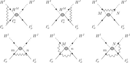
Figure 1: $W$ loop corrections to operators represented by the grey circle; there is also a current of external fermions $f$ present in the operator, but these lines are not drawn because they do not participate in the loop. These diagrams occur for all dimension eight operators; there are in addition wavefunction diagrams. Only the fourth diagram (without the Higgs legs), and wavefunction diagrams are present for dimension six operators. Superscripts are SU(2) indices, subscripts are flavour indices.

Consider first the diagrams of figure 1, which could contribute to the running and mixing of all dimension eight operators. The fermion wavefunction diagrams are $\propto\xi$ (the parameter of R-$\xi$ gauge), and the $W$ corrections to a scalar leg give a divergence

$$(-3+\xi)\frac{g^{2}}{4}[\tau^{a}\tau^{a}]_{IJ}\frac{i}{16\pi^{2}\epsilon}p^{2}~{}~{}~{}.$$ (III.1)

We systematically check that the coefficients of $\xi$ vanish in our calculation, so in the following, we drop all the diagrams which are proportional to $\xi$. Indeed, all the vertex diagrams in figure 1 are $\propto\xi$, so they do not contribute. Only the divergence from the scalar wavefunction remains, which renormalises operators but does not mix them among each other.

Figure 2: $W$ loops that can arise when the external fermion is an SU(2) doublet. Superscripts are SU(2) indices, subscripts are flavour indices.

When the external fermions are SU(2) doublets, for instance the first generation quark doublet $q_{1}$, additional diagrams arise. Firstly, there will be wavefunction corrections on the external doublet lines, and all but the third vertex diagram of figure 1 will occur, but with the $W$ attached to the external doublet line — these diagrams all vanish. In addition, there will be diagrams, illustrated in figure 2, where the $W$ is exchanged between the external fermion lines, and the flavour-changing lepton lines. These do not vanish, and correspond to the one-loop diagrams that renormalise and mix vector four-fermion operators.

The spinor contractions and momentum integral for the first two diagrams, at zero external momentum, give a divergence

$$-\frac{g^{2}}{4}\frac{C}{\Lambda_{NP}^{4}}\frac{i}{16\pi^{2}\epsilon}\times(3+\xi)(\overline{u}_{l}\gamma^{\alpha}P_{L}u_{k})(\overline{u}_{j}\gamma_{\alpha}P_{L}u_{i})$$ (III.2)

whereas the last two diagrams give the cancelling term $\propto\xi$. It remains to perform the SU(2) contractions, that define which operator mixes to which; these can be read off the anomalous dimension matrices given in section III.4.

For the case where there are identical fermions ($\ell_{e}$ as external fermions), the operator basis is smaller (see eqn II.14), so the divergences due to $W$ exchange among fermions look different. It is straightforward to check that the same divergences are generated by operators that become identical in the presence of identical fermions.

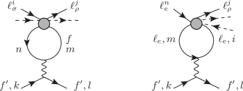
Figure 3: $W$ penguin diagrams that occur when the external fermion is a doublet. The right penguin only occurs if the operator involves identical fermions, such as two $\ell_{e}$ fields.

Finally, the $W$ bosons can mediate penguin diagrams, as illustrated in figure 3. For operators without identical fermions, only the left penguin can occur, and vanishes for ${\cal O}_{NSI}$, ${\cal O}_{H2}$ and ${\cal O}_{M2}$, due to a trace over the SU(2) generator. For $W$ penguins, there is only a sum over the colour of quarks in the loop, never a 2 for tracing over SU(2) doublets, because the loop vanishes as the trace of a generator in this case. These diagrams can change the external fermion, eg $\ell_{e}\leftrightarrow q_{1}$, thereby mixing operators with different external fermions; for simplicity, this mixing is neglected in the RGEs of section III.4. (It does not give additional constraints when the external fermion is a quark doublet; it is interesting for external lepton doublets and is briefly rediscussed in section IV.2.)

In the case of identical fermions (the external fermions are $\ell_{e}$, and $\rho$ or $\sigma$ is $e$), there could be two penguin diagrams, due to the identical fermions. However, since we consider vector operators, which can be rearranged according to Fierz, the spinor contractions and momentum integrals for the two possible diagrams are the same; only the SU(2) contractions can differ. In particular, the relative sign between the amplitudes is +, because the two diagrams are Fierz transformations of each other.

The different SU(2) contractions for the two penguin diagrams should correspond to the penguin contributions of two operators which become identical when there are identical fermions. For instance, for external $q$, ${\cal O}_{M2}$ has no penguin diagram, but ${\cal O}_{LQM2}$ generates divergences $\propto 2{\cal O}_{LQM2}-{\cal O}_{M2}$ via the penguin. For the operators with external $\ell_{e}$ and identical fermions, ${\cal O}_{M2}$ and ${\cal O}_{LQM2}$ are identical, so the “different” SU(2) contraction that allows ${\cal O}_{M2}$ to have a penguin diagram is just the SU(2) contraction that allowed a penguin to ${\cal O}_{LQM2}$. We conclude that in the reduced basis of operators with identical leptons, one must sum the penguin divergences of the different operators that become identical.

III.2 The Higgs loops

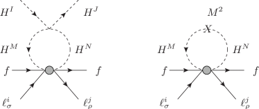
Figure 4: $H$ loops that mix and renormalise dimension eight operators, and mix them to dimension six via the Higgs $M^{2}$ insertion. The external fermion is $f$.

Closing the Higgs legs and inserting $\lambda H^{4}$ can renormalise and mix the dimension eight operators. Inserting instead $M^{2}$ on the scalar line, as in the right diagram of figure 4, mixes the dimension eight operators into ${\cal O}_{M2}$ and ${\cal O}_{LQM2}$. These loops are straightforward to calculate, have no subtleties in the presence of identical fermions, and give rise to the anomalous dimensions given in the following sections.

III.3 Deriving RGEs

We wish to obtain the one-loop RGEs for our operator coefficients, which, for a choice of lepton flavour indices $\rho,\sigma$, and external fermion $f$ are assembled in a row vector

$$\vec{C}=(C^{\rho,\sigma}_{NSI,f},C^{\rho,\sigma}_{H2,f},...,C^{\rho,\sigma}_{M2,f})~{}~{}~{},$$ (III.3)

where … is the additional coefficients that could arise if $f$ is an SU(2) doublet. It is convenient, during this derivation, to multiply ${\cal O}_{M2}$ and ${\cal O}_{LQM2}$ by $M^{2}$, so that all the operators are of dimension 8. With this modification, the Lagrangian in $4-2\epsilon$ dimensions can be expressed in terms of running fields and parameters as

$${\cal L} = ...+\frac{1}{\Lambda^{4}}\sum_{f}\left\{\vec{C}_{A}[Z]_{AB}\cdot(Z_{H}^{n/2}Z_{\ell}\mu^{(2+n)\epsilon}\vec{O}_{B})\right\}$$ (III.4)

where $n\in\{0,2\}$ is the number of Higgs legs of the operator $O_{B}$. The bare coefficients $\vec{C}_{bare}=\vec{C}[Z]\mu^{(2+n)\epsilon}$ should satisfy $\frac{d}{d\mu}\vec{C}_{bare}=0$, which gives Renormalisation Group Equations for the $C_{A}$s:

$$\mu\frac{\partial}{\partial\mu}{C}_{A} = -4\epsilon{C}_{A}+2\epsilon(\vec{C}\cdot[Z])_{M2}\delta_{A,M2}-\left(\vec{C}\cdot\mu\frac{\partial g_{i}}{\partial\mu}\frac{\partial[Z]}{\partial g_{i}}[Z]^{-1}\right)_{A}$$ (III.5)

$$= \vec{C}\cdot[\Gamma]$$ (III.6)

The operator $O_{M2}$ has dimension $8-4\epsilon$, whereas $O_{H2}$ and $O_{NSI}$ are $8-6\epsilon$-dimensional, which gives different ${\cal O}(\epsilon)$ terms in the RGEs. These terms give the anomalous dimensions mixing $O_{H2}$ and $O_{NSI}$ to $O_{M2}$, because the counterterms in the M2 column of $[Z]$ are independent of $\lambda$ and $g_{2}$, so the last term vanishes. As a result, the off-diagonal anomalous dimensions, as usual at one loop, are twice the coefficient of $1/\epsilon$ in the counterterms. For the diagonal anomalous dimensions, wavefunction contributions should be subtracted in the usual way (because the counterterms for an amputated operator are represented by $\vec{C}\cdot\ [C]=\vec{C}\cdot\ [Z]Z_{H}^{n/2}Z_{\ell}$, but we only want $[Z]$):

$$[\Gamma]_{AA} = 2[C^{(1)}]_{AA}-2Z^{(1)}_{\ell}-2Z^{(1)}_{H}\delta_{1,n/2}$$ (III.7)

$${[\Gamma]}_{AB} = 2[C^{(1)}]_{AB}~{}~{}~{},~{}~{}~{}~{}A\neq B$$

where $Z^{(1)}$ is the coefficient of $1/\epsilon$ in $Z$.

Neglecting the running of the couplings ($g_{2}$,$y_{t}$, $\lambda$), the solution is

$$\vec{C}(\mu_{f}) = \vec{C}(\mu_{i})\cdot\left([I]+[\Gamma]\log\frac{\mu_{f}}{\mu_{i}}+\frac{1}{2}[\Gamma\Gamma]\log^{2}\frac{\mu_{f}}{\mu_{i}}+...\right)$$ (III.8)

where, by analogy with running masses, the couplings in $[\gamma]$ are to be evaluated at $\mu_{f}$.

III.4 The anomalous dimension matrix

For singlet external fermions, in the basis $(C_{NSI},C_{H2},C_{M2})$, the anomalous dimension matrix is

$$[\Gamma] = \frac{g^{2}}{4\kappa}\left[\begin{array}[]{ccc}-18&0&0\\ 0&-18&0\\ 0&0&0\\ \end{array}\right]+\frac{1}{\kappa}\left[\begin{array}[]{ccc}-4\lambda&2\lambda&-2\eta\\ 2\lambda&-4\lambda&2\eta\\ 0&0&0\\ \end{array}\right]$$ (III.19)

$$+\frac{g^{{}^{\prime}2}}{4\kappa}\left[\begin{array}[]{ccc}-6+24Y_{f}+16N_{c}Y_{f}^{2}/3&0&0\\ 0&-6+24Y_{f}+16N_{c}Y_{f}^{2}/3&0\\ 0&0&24Y_{f}+16N_{c}Y_{f}^{2}/3\\ \end{array}\right]~{}~{}$$

$${[\Gamma\Gamma]} = \frac{1}{\kappa^{2}}\left[\begin{array}[]{ccc}d^{2}+4\lambda^{2}&4\lambda d&4\lambda\eta-2\eta(d+d^{\prime})\\ 4\lambda d&d^{2}+4\lambda^{2}&-4\lambda\eta+2\eta(d+d^{\prime})\\ 0&0&d^{{}^{\prime}2}\\ \end{array}\right]$$ (III.23)

where $\kappa=16\pi^{2}$, $\eta=M^{2}/\Lambda^{2}$, and $d=-(9g^{2}/2+4\lambda+g^{{}^{\prime}2}[1.5-6Y_{f}-4N_{c,f}Y_{f}^{2}/3])\sim-4$ is the diagonal anomalous dimension of ${\cal O}_{NSI}$ and ${\cal O}_{H2}$, and $d^{\prime}$ that of ${\cal O}_{M2}$.

For doublet external fermions, in the basis $(C_{NSI},C_{H2},(C_{CCLFV}+C_{CCLFV}^{\dagger})/2,(C_{CCNSI}+C_{CCNSI}^{\dagger})/2$, $(C_{CCLFV}-C_{CCLFV}^{\dagger})/2$, $C_{LQM2},C_{M2})$, the anomalous dimension matrix is

$$[\Gamma] = -\frac{3g^{2}}{\kappa}\left[\begin{array}[]{ccccccccc}\frac{5}{2}&0&0&-1&0&0&0\\ 0&\frac{5}{2}&-1&0&0&0&0\\ 2&-2&\frac{3}{2}&-1&0&0&0\\ -2&2&-1&\frac{3}{2}&0&0&0\\ 0&0&0&0&\frac{5}{2}&0&0\\ 0&0&0&0&0&1&-2\\ 0&0&0&0&0&-2&1\\ \end{array}\right]$$ (III.46)

$$+\frac{g^{2}N_{c}}{3\kappa}\left[\begin{array}[]{ccccccccc}0&0&0&0&0&0&0\\ 0&0&0&0&0&0&0\\ 0&-2&2&0&0&0&0\\ -2&0&0&2&0&0&0\\ 0&0&0&0&2&0&0\\ 0&0&0&0&0&2&-1\\ 0&0&0&0&0&0&0\\ \end{array}\right]+\frac{1}{\kappa}\left[\begin{array}[]{ccccccccc}-4\lambda&2\lambda&0&0&0&0&-2\eta\\ 2\lambda&-4\lambda&0&0&0&0&2\eta\\ 0&0&-4\lambda&2\lambda&0&4\eta&0\\ 0&0&2\lambda&-4\lambda&0&-4\eta&0\\ 0&0&0&0&-2\lambda&0&0\\ 0&0&0&0&0&0&0\\ 0&0&0&0&0&0&0\\ \end{array}\right]$$

where $\kappa=16\pi^{2}$, $\eta=M^{2}/\Lambda^{2}$, and the first matrix is from $W$ exchange, the second is the $W$ penguins and the last is the Higgs.

In the case with external lepton doublets and identical fermions, several operators are identical (see eqn II.12), so the anomalous dimension mixing operator A into operator B is the $\sum_{B^{\prime}}\Gamma_{AB^{\prime}}$ over all the operators $\{B^{\prime}\}$ who are identical to $B$. This rule applies to the second matrix of eqn(III.46). Then for the penguins, the rule is to sum also over the identical operators in the column: $\Gamma_{AB}=\sum_{A^{\prime},B^{\prime}}\Gamma_{A^{\prime}B^{\prime}}$. Then the anomalous dimension matrix, in the basis $(C_{NSI},C_{H2},C_{CCNSI+},C_{M2})$, is

$$[\Gamma] = -\frac{3g^{2}}{\kappa}\left[\begin{array}[]{cccc}\frac{5}{2}&0&-1&0\\ 2&\frac{1}{2}&-1&0\\ 0&0&\frac{1}{2}&0\\ 0&0&0&-1\\ \end{array}\right]+\frac{g^{2}N_{c}}{3\kappa}\left[\begin{array}[]{cccc}1&0&0&0\\ 0&1&0&0\\ -5&1&4&0\\ 0&0&0&1\\ \end{array}\right]+\frac{1}{\kappa}\left[\begin{array}[]{cccc}-4\lambda&2\lambda&0&-2\eta\\ 2\lambda&-4\lambda&0&2\eta\\ -4\lambda&+4\lambda&-2\lambda&-4\eta\\ 0&0&0&0\\ \end{array}\right]~{}~{}$$ (III.59)

IV Results

This section presents the LFV that is induced by electroweak loop corrections to NSI operators. Section IV.1 summarises relevant experimental constraints on LFV, then section IV.2 applies these constraints to the LFV coefficients induced by loop corrections to NSI. Possible cancellations allowing to avoid these constraints are discussed in section IV.3.

IV.1 Experimental sensitivity to LFV operators

Loop corrections to NSI can induce vector four-fermion operators (as given in eqn II.15), that involve two charged leptons of different flavour, and two first generation fermions $e,u,$ or $d$. This section lists the experimental sensitivity to such coefficients. Since all the operators considered here are hermitian (on doublet lepton flavour indices $\rho\sigma$), we do not distinguish between bounds on $C^{\rho\sigma ff}$ vs $C^{\sigma\rho ff}$, and quote bounds on only one.

If the lepton flavours $\rho,\sigma$ are $\mu$ and $e$, then $\mu\to e\bar{e}e$ and $\mu\!\to\!e~{}{\rm conversion}$ are sensitive to the LFV induced by loop corrections to NSI operators. Current bounds from SINDRUM Bellgardt:1987du ; Bertl:2006up at 90$\%$ C.L. are $BR(\mu Au\to eAu)\leq 7.0\times 10^{-13}$, and $BR(\mu\to e\bar{e}e)\leq 10^{-12}$, and give sensitivities (to the operator coefficients at $m_{W}$)

$$C^{\mu eee}_{V,LL} \leq 7.8\times 10^{-7}$$ (IV.1)

$$C^{\mu eee}_{V,LR} \leq 9.3\times 10^{-7}$$ (IV.2)

$$C^{\mu edd}_{V,LL} \leq 5.3\times 10^{-8}$$ (IV.3)

$$C^{\mu edd}_{V,LR} \leq 5.4\times 10^{-8}$$ (IV.4)

$$C^{\mu euu}_{V,LL} \leq 6.0\times 10^{-8}$$ (IV.5)

$$C^{\mu euu}_{V,LR} \leq 6.3\times 10^{-8}$$ (IV.6)

Experiments under construction (COMET COMET ,Mu2e Mu2e ,Mu3e Mu3e ) will improve these sensitivities by two orders of magnitude in a few years.

For one of $\rho,\sigma$ a $\tau$, and the other $\mu$ or $e$, current bounds on $\tau\to\ell e^{+}e^{-}$ at 90$\%$ C.L. give dim52

$$C^{\tau eee}_{V,LL} \leq 2.8\times 10^{-4}$$ (IV.7)

$$C^{\tau eee}_{V,LR} \leq 4.0\times 10^{-4}$$ (IV.8)

$$C^{\tau\mu ee}_{V,LL} \leq 3.2\times 10^{-4}$$ (IV.9)

$$C^{\tau\mu ee}_{V,LR} \leq 3.2\times 10^{-4}~{}~{}.$$ (IV.10)

These sensitivities again apply to the operator coefficients at $m_{W}$.

The operators with $u$ or $d$ quarks as external fermions can be probed by the LFV $\tau$ decays $BR(\tau\to\{\mu,e\}\pi^{0})\leq\{1.1\times 10^{-7},8\times 10^{-8}\}$ tmp ; tep , $BR(\tau\to\{\mu,e\}\rho)\leq\{1.2\times 10^{-8},1.8\times 10^{-8}\}$ tlr and $BR(\tau\to\{\mu,e\}\eta)\leq\{6.5\times 10^{-8},9.2\times 10^{-8}\}$ tep (all limits at 90$\%$ C.L.). As noted in BHHS , these three decays given complementary constraints, because the $\eta$ is an isospin singlet ($\propto\bar{u}\Gamma u+\bar{d}\Gamma d$) whereas the pion and $\rho$ are isotriplets($\propto\bar{u}\Gamma u-\bar{d}\Gamma d$), and the decays to pions or $\rho$s are respectively sensitive to LFV operators involving the axial or vector quark current.

It is convenient to normalise the pion decays to the SM process $\tau\to\nu\pi^{-}$ (with $BR(\tau\to\nu\pi^{-})=0.108$PDB ), in order to cancel the hadronic and phase space factors:

$$\frac{BR(\tau\to\ell\pi^{0})}{BR(\tau\to\nu\pi^{-})}=\frac{|C^{\tau\ell uu}_{V,LR}-C^{\tau\ell uu}_{V,LL}-C^{\tau\ell dd}_{V,LR}+C^{\tau\ell dd}_{V,LL}|^{2}}{2|V_{ud}|^{2}}$$ (IV.11)

where the $2$ is because $\sqrt{2}\langle 0|\overline{u}\gamma^{\alpha}\gamma_{5}u|\pi_{0}\rangle=\langle 0|\overline{u}\gamma^{\alpha}\gamma_{5}d|\pi^{-}\rangle$. This gives

$$|C^{\tau euu}_{V,LR}-C^{\tau euu}_{V,LL}-C^{\tau edd}_{V,LR}+C^{\tau edd}_{V,LL}| \leq 1.2\times 10^{-3}$$

$$|C^{\tau\mu uu}_{V,LR}-C^{\tau\mu uu}_{V,LL}-C^{\tau\mu dd}_{V,LR}+C^{\tau\mu dd}_{V,LL}| \leq 1.4\times 10^{-3}~{}~{}.$$ (IV.12)

These sensitivities apply to the coefficients at the experimental scale (not the weak scale as for eqns IV.10 and IV.6).

The trick of normalising by an SM decay is more subtle in the case of $\tau\to\ell\rho$, because the $\rho$ decays to two pions, so the $\tau\to\ell\rho$ bounds are obtained by selecting a range of $\pi^{+}\pi^{-}$ invariant-mass-squared appropriate for the $\rho(770)$. The corresponding SM decay is $BR(\tau\to\nu\pi^{0}\pi^{-})=.255$, studied by Belle Belletnpp over a wide invariant-mass-squared. The fit to the spectrum performed by Belle suggests that $\sim 80\%$ of the events are due to the $\rho(770)$, so for simplicity we suppose:

$$\frac{BR(\tau\to\ell\rho)}{BR(\tau\to\nu\pi^{0}\pi^{-})}=\frac{|C^{\tau\ell uu}_{V,LR}+C^{\tau\ell uu}_{V,LL}-C^{\tau\ell dd}_{V,LR}-C^{\tau\ell dd}_{V,LL}|^{2}}{2}$$ (IV.13)

which gives

$$|C^{\tau euu}_{V,LR}+C^{\tau euu}_{V,LL}-C^{\tau edd}_{V,LR}-C^{\tau edd}_{V,LL}| \leq 3.8\times 10^{-4}$$

$$|C^{\tau\mu uu}_{V,LR}+C^{\tau\mu uu}_{V,LL}-C^{\tau\mu dd}_{V,LR}-C^{\tau\mu dd}_{V,LL}| \leq 3.1\times 10^{-4}~{}~{}.$$ (IV.14)

For the $\eta$, we approximate $f_{\eta}\simeq F_{\pi}\simeq 92$ MeV (see feta for a detailed discussion), so that

$$\frac{\Gamma(\tau\to\ell\eta)}{\Gamma(\tau\to\nu\pi^{-})}=\frac{|C^{\tau\ell uu}_{V,XR}-C^{\tau\ell uu}_{V,XL}+C^{\tau\ell dd}_{V,XR}-C^{\tau\ell dd}_{V,XL}|^{2}}{2}~{}~{}~{},$$ (IV.15)

and the current bounds on $\Gamma(\tau\to\ell\eta)$ imply

$$|C^{\tau euu}_{V,XR}-C^{\tau euu}_{V,XL}+C^{\tau edd}_{V,XR}-C^{\tau edd}_{V,XL}| \leq 6.5\times 10^{-4}$$

$$|C^{\tau\mu uu}_{V,XR}-C^{\tau\mu uu}_{V,XL}+C^{\tau\mu dd}_{V,XR}-C^{\tau\mu dd}_{V,XL}| \leq 5.4\times 10^{-4}~{}~{}.$$ (IV.16)

In coming years, Belle II could improve the sensitivity to LFV $\tau$ decays by one or two orders of magnitude Kou:2018nap .

For models that induce LFV on left-handed, or right-handed quarks, but not both, the bounds of eqns (IV.14) and (IV.16) can be combined in a covariance matrix to obtain

$$|C^{\tau eqq}_{V,LX}| \leq 7.1\times 10^{-4}$$

$$|C^{\tau\mu qq}_{V,LX}| \leq 5.9\times 10^{-4}$$ (IV.17)

where $q\in\{u,d\}$ and $X=L$ or $R$.

IV.2 LFV due to NSI

We consider combinations of operator coefficients which, at tree level, induce NSI but not LFV (these were given section II), and use the RGEs obtained in section III to estimate the effect of loops. For example, the one-loop [or two-loop] mixing of a given combination of tree-level coefficients, can be obtained from the second [or third] term of eqn (III.8), with $\vec{C(\mu_{i})}$ the input (tree) coefficients at the New Physics scale $\mu_{i}=\Lambda_{NP}$, and $\vec{C(\mu_{f})}$ the loop-induced combination at the weak scale $m_{W}$. By matching $\vec{C(\mu_{f})}$ onto the low-energy theory, one obtains the LFV induced by the one-loop RGEs.

The case of singlet external fermions is simple to discuss as an explicit example. Eqn (II.16) implies that NSI can arise at tree-level from $C_{NSI}$ and/or $C_{M2}$ (subdominant loop contributions to coefficients induced at tree level are neglected in the following.) For only $C_{NSI}(\Lambda_{NP})\neq 0$, eqn (III.19) gives

$$\Delta C^{\rho\sigma}_{H2,f}(m_{W}) = C^{\rho\sigma}_{NSI,f}(\Lambda_{NP})\times\left(\frac{2\lambda}{(16\pi^{2})}\log\frac{\Lambda_{NP}}{m_{W}}+\frac{4\lambda d}{2(16\pi^{2})^{2}}\log^{2}\frac{\Lambda_{NP}}{m_{W}}+...\right)$$

$$\Delta C^{\rho\sigma}_{M2,f}(m_{W}) = C_{NSI,f}^{\rho\sigma}(\Lambda_{NP})\times\left(-\frac{2\eta}{(16\pi^{2})}\log\frac{\Lambda_{NP}}{m_{W}}+\frac{4\lambda\eta-2\eta(d+d^{\prime})}{2(16\pi^{2})^{2}}\log^{2}\frac{\Lambda_{NP}}{m_{W}}+...\right)$$

where $d$ and $d^{\prime}$ are defined after eqn (III.19). Matching onto the low-energy operators according to eqn (II.16) with table 1, gives, at first order in $1/(16\pi^{2})$, a vanishing LFV coefficient $C_{V,LR}^{\rho\sigma ff}=0$, due to potential minimisation conditions. However, at second order in the one-loop RGEs, ${\cal O}_{NSI}$ induces LFV at low energy:

$$\Delta C_{V,LR}^{\rho\sigma ff}=\frac{C^{\rho\sigma}_{NSI,f}(\Lambda_{NP})v^{4}}{\Lambda_{NP}^{4}}\frac{2\lambda(d-d^{\prime})+4\lambda^{2}}{2(16\pi^{2})^{2}}\log^{2}\frac{\Lambda_{NP}}{m_{W}}\sim 10^{-4}\varepsilon_{f}~{}~{}~{},$$ (IV.18)

where $d-d^{\prime}=-(9g^{2}/2+4\lambda)$ if hypercharge is neglected, and for the numerical estimates in this section, we conservatively take $\Lambda_{NP}\sim 250-300$ GeV in the logarithm.

For $C_{M2}(\Lambda_{NP})\neq 0$, the tree contribution to LFV must be cancelled by $C_{H2}(\Lambda_{NP})=-(\lambda/\eta)C_{M2}(\Lambda_{NP})$ as given in eqn (II.17). Then the RGEs generate corrections to $C_{H2}$ and $C_{M2}$:

$$\Delta C^{\rho\sigma}_{H2,f}(m_{W}) = C^{\rho\sigma}_{H2,f}(\Lambda_{NP})\times\frac{d}{(16\pi^{2})}\log\frac{\Lambda_{NP}}{m_{W}}+...$$

$$\Delta C^{\rho\sigma}_{M2,f}(m_{W}) = C_{M2}(\Lambda_{NP})\times\frac{d^{\prime}-2\lambda}{(16\pi^{2})}\log\frac{\Lambda_{NP}}{m_{W}}+...$$

which match onto low-energy LFV at one loop:

$$\Delta C_{V,LR}^{\rho\sigma ff}=\frac{C_{M2}(\Lambda_{NP})v^{2}}{(16\pi^{2})\Lambda_{NP}^{2}}\left[-(d-d^{\prime})-2\lambda\right]\log\frac{\Lambda_{NP}}{m_{W}}\sim-2\times 10^{-2}\varepsilon_{f}~{}~{}~{}.$$ (IV.19)

So a heavy New Physics model that gives NSI on singlet fermions will induce LFV via loops, which is the sum of eqns (IV.19) and (IV.18).

Figure 5: The loop-induced LFV coefficient, normalised to the NSI coefficient $\varepsilon_{f}$, for SU(2) singlet external fermions $f$, as a function of the ratio of the two independent operator coefficients that can induce NSI: $C_{M2}(\Lambda_{NP})$ and $C_{NSI}(\Lambda_{NP})$. $C_{H2}(\Lambda_{NP})$ is determined as a function of $C_{M2}(\Lambda_{NP})$ by the cancellation of tree-LFV given in eqn (II.17). The left plot is for negative $C_{M2}/C_{NSI}$, and positive values are in the plot to the right.

In figures 5, the magnitude of the LFV coefficient is plotted against the ratio $C_{M2,f}\Lambda^{2}/C_{NSI,f}v^{2}$, for $\varepsilon_{f}=1.0$ and assuming tree-level LFV cancels according to eqn (II.17). For $|C_{M2,f}|>|C_{NSI,f}v^{2}/\Lambda^{2}|$, it is clear from eqns (II.16,IV.19,IV.18) that $\varepsilon_{f}\simeq-C_{M2,f}v^{2}/\Lambda^{2}$, and $C_{V,LR}\simeq-2\times 10^{-2}\varepsilon_{f}$, so the plots illustrate the regions $|C_{M2,f}|<|C_{NSI,f}v^{2}/\Lambda^{2}|$ (For $C_{M2,f}=C_{NSI,f}v^{2}/\Lambda^{2}$, $\varepsilon_{f}$ vanishes so $C_{V,LR}/\varepsilon_{f}$ diverges.). At $C_{M2,f}=C_{NSI,f}v^{2}\ln/(32\pi^{2}\Lambda^{2})$, the figure shows an “accidental” cancellation between the contributions to the LFV coefficient from eqns (IV.19) and (IV.18); we are reluctant to admit this loophole in the LFV constraints on NSI, because it is difficult to build models that tune Lagrangian parameters against logarithms of mass scales.

The experimental bounds on LFV from section IV.1 can now be applied to the loop-induced LFV coefficient, obtained by summing eqns (IV.19) and (IV.18). This gives an upper bound on the NSI coefficient, that depends on the ratio $\Lambda^{2}C_{M2}/(v^{2}C_{NSI})$ : $\varepsilon_{f}^{\rho\sigma}\times$ the value given in the plot must be smaller than the experimental constraint. For instance, for $C_{M2}(\Lambda)\mathrel{\vbox{\hbox{$<$}\nointerlineskip\hbox{$\sim$}}}10^{-2}C_{NSI}(\Lambda)$, $\varepsilon_{f}^{\mu e}$ must be $<10^{-3}\to 10^{-2}$ as given in the first column of table 2, and $\tau\leftrightarrow e,\mu$ NSI can be ${\cal O}(1)$. The $\tau$ decay bounds are given in the second two columns of table 2. On the other hand, as soon as $C_{M2}$ strays away from 0, the LFV bounds on NSI are more restrictive (this is illustrated in figure 5) — then the LFV is ${\cal O}(10^{-2}\varepsilon_{f})$, and the constraints on LFV are given in table 3. Notice however, that all these estimates are approximate because our EFT calculation only allows to obtain the logⁿ-enhanced part of $n$-loop diagrams, and since the logarithm cannot be large, our results should give the order of magnitude, but not two significant figures.

$\varepsilon_{e_{R}}^{\mu e}\mathrel{\vbox{\hbox{$<$}\nointerlineskip\hbox{$\sim$}}}9\times 10^{-3}$	$\varepsilon_{e_{R}}^{\tau e}\mathrel{\vbox{\hbox{$<$}\nointerlineskip\hbox{$\sim$}}}4$	$\varepsilon_{e_{R}}^{\tau\mu}\mathrel{\vbox{\hbox{$<$}\nointerlineskip\hbox{$\sim$}}}3$
$\varepsilon_{u_{R}}^{\mu e}\mathrel{\vbox{\hbox{$<$}\nointerlineskip\hbox{$\sim$}}}5\times 10^{-4}$	$\varepsilon_{u_{R}}^{\tau e}\mathrel{\vbox{\hbox{$<$}\nointerlineskip\hbox{$\sim$}}}7$	$\varepsilon_{u_{R}}^{\tau\mu}\mathrel{\vbox{\hbox{$<$}\nointerlineskip\hbox{$\sim$}}}6$
$\varepsilon_{d_{R}}^{\mu e}\mathrel{\vbox{\hbox{$<$}\nointerlineskip\hbox{$\sim$}}}6\times 10^{-4}$	$\varepsilon_{d_{R}}^{\tau e}\mathrel{\vbox{\hbox{$<$}\nointerlineskip\hbox{$\sim$}}}7$	$\varepsilon_{d_{R}}^{\tau\mu}\mathrel{\vbox{\hbox{$<$}\nointerlineskip\hbox{$\sim$}}}6$

Table 2: Bounds on flavour-changing NSI parameters from the non-observation of LFV processes among charged leptons, obtained from eqn (IV.18) for SU(2) singlet external fermions. Comparable limits apply to to the $\{\varepsilon_{fL}^{\rho\sigma}\}$ for doublets, as discussed after eqn (IV.20). These bounds, which are almost unavoidable, arise from two-loop contributions (${\cal O}(\alpha^{2}\log^{2}$)) of the NSI operators to LFV processes.

$\varepsilon_{e_{R}}^{\mu e}\mathrel{\vbox{\hbox{$<$}\nointerlineskip\hbox{$\sim$}}}5\times 10^{-5}$	$\varepsilon_{e_{R}}^{\tau e}\mathrel{\vbox{\hbox{$<$}\nointerlineskip\hbox{$\sim$}}}2\times 10^{-2}$	$\varepsilon_{e_{R}}^{\tau\mu}\mathrel{\vbox{\hbox{$<$}\nointerlineskip\hbox{$\sim$}}}2\times 10^{-2}$
$\varepsilon_{u_{R}}^{\mu e}\mathrel{\vbox{\hbox{$<$}\nointerlineskip\hbox{$\sim$}}}3\times 10^{-6}$	$\varepsilon_{u_{R}}^{\tau e}\mathrel{\vbox{\hbox{$<$}\nointerlineskip\hbox{$\sim$}}}4\times 10^{-2}$	$\varepsilon_{u_{R}}^{\tau\mu}\mathrel{\vbox{\hbox{$<$}\nointerlineskip\hbox{$\sim$}}}3\times 10^{-2}$
$\varepsilon_{d_{R}}^{\mu e}\mathrel{\vbox{\hbox{$<$}\nointerlineskip\hbox{$\sim$}}}3\times 10^{-6}$	$\varepsilon_{d_{R}}^{\tau e}\mathrel{\vbox{\hbox{$<$}\nointerlineskip\hbox{$\sim$}}}4\times 10^{-2}$	$\varepsilon_{d_{R}}^{\tau\mu}\mathrel{\vbox{\hbox{$<$}\nointerlineskip\hbox{$\sim$}}}3\times 10^{-2}$

Table 3: Bounds on flavour-changing NSI parameters from the non-observation of LFV processes among charged leptons, obtained from eqn (IV.19) for NSI on SU(2) singlet external fermions. Comparable limits apply to to the $\{\varepsilon_{fL}^{\rho\sigma}\}$ for doublets, as discussed after eqn (IV.20). These bounds arise from one-loop contributions (${\cal O}(\alpha\log$)) of the NSI operators to LFV processes, and can be avoided in models that generate particular patterns of coefficients as discussed in the text.

If the external fermion is an SU(2) doublet, the situation is more involved. It is again the case that $C_{NSI}$ first mixes into LFV at ${\cal O}(\alpha^{2}\log^{2}$), but for external doublet quarks, the other five coefficients all induce LFV at ${\cal O}(\alpha\log$) . In order to avoid tree-level LFV, those five coefficients must satisfy two constraints, obtained by setting eqns (II.19) to zero. Then they will induce LFV as given by the RGEs of eqn (III.46):

$$\Delta C^{\rho\sigma uu}_{V,LL} = \frac{v^{2}}{\Lambda^{2}}\frac{\log(\Lambda/m_{W})}{16\pi^{2}}\left([\frac{9}{2}g^{2}+2\lambda]C^{\rho\sigma}_{M2,q}-6g^{2}\frac{v^{2}}{\Lambda^{2}}C^{\rho\sigma}_{CCNSI+,q}+g^{2}C^{\rho\sigma}_{LQM2,q}\right)$$

$$\Delta C^{\rho\sigma dd}_{V,LL} = \frac{v^{2}}{\Lambda^{2}}\frac{\log(\Lambda/m_{W})}{16\pi^{2}}\left(C^{\rho\sigma}_{M2,q}+C^{\rho\sigma}_{LQM2,q}\right)[\frac{9}{2}g^{2}+2\lambda]$$ (IV.20)

If NSI are due to some subset of $C_{CCNSI+,q}$, $C_{M2,q}$ and $C_{LQM2,q}$, and the LFV coefficients of eqn (IV.20) do not vanish, then the bounds of table 3 would generically apply. (We do not make plots in this case, because there are four independent coefficients).

On the other hand, the above equations contain three coefficients, so it is possible for the New Physics model to arrange them such that the ${\cal O}(\alpha\log)$ LFV on $u_{L}$ and $d_{L}$ currents vanishes: the coefficients $C_{H2,q}$, $C_{CCLFV+,q}$, $C_{CCNSI+,q}$, $C_{M2,q}$ and $C_{LQM2,q}$ must all be non-zero, and satisfy the four relations obtained by setting eqns (IV.20) and (II.19) to vanish. If a model could be constructed to implement this cancellation, it is possible that there would be not-log-enhanced one-loop contributions to LFV operators; however, to verify that in EFT would require going beyond our leading-log analysis. It is however sure, from our one-loop RGEs, that LFV will be induced at ${\cal O}(\alpha^{2}\log^{2})$, so that constraints of order those in table 2 would apply. As in the case of external SU(2)-singlet fermions, these constraints also apply if the model matches only onto ${\cal O}_{NSI,q}$ at the scale $\Lambda$, with all the other coefficients relatively suppressed by $\sim 10^{-2}$. The exact formulae for these ${\cal O}(\alpha^{2}\log^{2})$ contributions are straightforward to obtain from the third term in eqn (III.8); they are not quoted here because they are lengthy.

It is interesting to resurrect the “external-fermion-changing” $W$-penguin diagrams of figure 3, before giving results for the case where the external fermion is a lepton doublet. These penguins can change the external fermion $\ell_{e}\leftrightarrow q$, so, for instance, an operator with external $\ell_{e}$ could generate one-loop LFV on $u_{L}$ and $d_{L}$. Requiring that the model choose its parameters to cancel this LFV gives an additional constraint on NSI for doublet leptons when $\rho\sigma\in\{\mu,\tau\}$ that is given in eqn (IV.22).

For external $\ell_{e}$, the NSI and LFV are different if one of $\rho,\sigma$ is first generation. When yes, tree level NSI and LFV are respectively generated by the coefficient combinations given in eqns (II.22) and (II.17). For $\rho,\sigma\in\{\mu,\tau\}$, the combinations are given in eqns (II.21) and (II.20). In the following, we suppose that the tree-LFV combinations of eqns (II.17) and (II.21) vanish.

The operator ${\cal O}_{NSI,\ell}$, which contributes to tree-level NSI, first induces LFV at ${\cal O}(\alpha^{2}\log^{2})$. NSI can also arise due to $C_{M2,\ell}$, in which case the one-loop LFV is different depending if one of $\rho,\sigma$ is first generation. When yes, then the one-loop LFV on electrons is:

$$\Delta C^{\rho\sigma ee}_{V,LL} = \frac{v^{2}}{\Lambda^{2}}\frac{\log(\Lambda/m_{W})}{16\pi^{2}}\left([\frac{15}{2}g^{2}+2\lambda]C^{\rho\sigma}_{M2,\ell}+\frac{g^{2}}{3}C^{\rho\sigma}_{CCNSI+,\ell}\right)~{}~{}~{},$$ (IV.21)

and the $W$-penguin-induced LFV on quarks vanishes when eqn (II.17) does. So if NSI are induced by $C_{M2,\ell}$, then the model can tune coefficients to cancel tree and one-loop LFV, by ensuring that eqns (II.17) and (IV.21) vanish.

For $\rho$ and $\sigma\in\{\mu,\tau\}$, the one-loop LFV is induced on $u_{L}$ and $d_{L}$ by the $W$ penguins

$$\Delta C^{\rho\sigma uu}_{V,LL} = \frac{g^{2}}{3}\frac{v^{2}}{\Lambda^{2}}\frac{\log(\Lambda/m_{W})}{16\pi^{2}}\left(\frac{\eta}{\lambda}C^{\rho\sigma}_{H2,\ell}+C^{\rho\sigma}_{M2,\ell}\right)$$

$$\Delta C^{\rho\sigma dd}_{V,LL} = \frac{g^{2}}{3}\frac{v^{2}}{\Lambda^{2}}\frac{\log(\Lambda/m_{W})}{16\pi^{2}}\left(2\frac{\eta}{\lambda}C^{\rho\sigma}_{CCLFV+,\ell}+C^{\rho\sigma}_{LQM2,\ell}\right)$$ (IV.22)

and on leptons:

$$\Delta C^{\rho\sigma ee}_{V,LL} = \frac{v^{2}}{\Lambda^{2}}\frac{\log(\Lambda/m_{W})}{16\pi^{2}}\left([\frac{9}{2}g^{2}+2\lambda](C^{\rho\sigma}_{M2,\ell}+C^{\rho\sigma}_{LQM2,\ell})+\frac{g^{2}}{3}C^{\rho\sigma}_{LQM2,\ell}+\frac{2}{3}g^{2}\frac{v^{2}}{\Lambda^{2}}C^{\rho\sigma}_{CCLFV+,\ell}\right)$$ (IV.23)

So if NSI arise due to an operator other than ${\cal O}_{NSI}$, then at least two coefficients must be cancel against each other to avoid tree LFV(as shown in eqn II.21), and LFV will arise at one loop unless the model arranges eqns (IV.23,IV.22) to vanish.

In summary, for external lepton doublets, the LFV constraints are similar the case of an external quark doublet: generically, the bounds of table 3 would apply; in the case where the model matches only onto ${\cal O}_{NSI}$, or where it arranges its coefficients to cancel the LFV at ${\cal O}(\alpha\log)$, then the bounds of 2 would apply.

IV.3 Cancellations

The results given in tables 3 and 2 are not in reality “bounds” on NSI from LFV processes, but rather “sensitivities”: NSI coefficients larger than the given value could mediate LFV rates above the experimental limit, but not necessarily, in the case where their contribution to LFV is cancelled by other coefficients. This section lists some possible cancellations that could allow NSI to evade the LFV constraints.

1. As already discussed, for external fermions that are SU(2) doublets, there are enough operators such that, not only the combination of coefficients which contributes at tree level to LFV can be chosen to vanish, but also the coefficient combination that contributes at $\alpha\log$. But the two-loop ${\cal O}(\alpha^{2}\log^{2})$ bounds of table 2 would still apply.

2. We neglected possible cancellations between flavours or chiralities of quarks in the experimental sensitivities of section IV.1.

   In the case of NSI involving $\tau\leftrightarrow\ell$ flavour change, the $\tau$ decay bounds quoted do not constrain the isosinglet vector combination $C_{V,XL}^{\tau\ell uu}+C_{V,XR}^{\tau\ell uu}+C_{V,XL}^{\tau\ell dd}+C_{V,XR}^{\tau\ell dd}$. The authors are unaware of restrictive bounds on this combination; if indeed they are absent, then tree LFV bounds for $\tau\leftrightarrow\ell$ NSI would not apply to an NSI model where the low-energy LFV coefficients are equal for external fermions $f=q_{L},u_{R},d_{R}$. This equality could substitute for imposing the tree cancellations of eqn (II.19). However, the coefficients of operators with external fermions $q$,$u_{R}$ and $d_{R}$ all run differently (the last two due to different hypercharge), so LFV would still arise at one loop, and the one-loop bounds would apply, unless further cancellations are arranged.

   In the case of $\mu\leftrightarrow e$ NSI, the $\mu\to e$ conversion bounds apply to a weighted sum of the $u$ and $d$ vector currents, where the weighting factor depends on the target nucleus. It is not possible to avoid the bound by cancelling $u$ vs $d$ coefficients, because there are restrictive bounds on $\mu\to e$ conversion on Gold (Z=79, used to obtain eqn IV.6) and Titanium (Z=22, $BR(\mu Ti\to eTi)\leq 4.2\times 10^{-12}$), which have different $n/p$ ratios, so together constrain the $u-d$ combination a factor of 2 less well than $u+d$. However, the sensitivity of $\mu\to e$ conversion to the axial vector LFV operator $(\overline{e}\gamma^{\alpha}P_{L}\mu)(\overline{q}\gamma_{\alpha}\gamma_{5}q)$, is $\sim$ three orders of magnitude weaker (below $m_{W}$, the axial vector mixes via the RGEs of QED to the vector operator). So if loop corrections to NSI generated LFV on the axial quark current, the LFV bound on NSI would be weakened by $10^{3}$.

   This requires NSI on doublet and singlet quarks (involving operators other than ${\cal O}_{NSI}$), whose coefficients satisfy the zero-tree-LFV conditions, and where the external doublet coefficients are of comparable magnitude and opposite sign to the singlet coefficients. Then U(1) and SU(2) penguin diagrams, that could mix these operators to those with external electrons, vanish due to the zero-tree-LFV condition, and the bounds in the second and third row of the first column of table 2 could be relaxed by three orders of magnitude.

3. We neglected the possibility that the model induces “other” LFV not included in our subset of operators (for instance, tensor or scalar four-fermion operators), that could mix into it and cause cancellations at low energy.

4. We do not allow cancellations between Wilson coefficients at $\Lambda$ (expressed in terms of parameters of the high-scale theory), against other Wilson coefficients multiplied by log$(v/\Lambda)$, because this would be “unnatural” in EFT (In principle, the model predicts the couplings, but the observer chooses the scale at which experiments are done, and therefore the ratio in the log.). However, such “accidental” cancellations can occur and be numerically important; an example would be a model whose coefficients sit in the valley of figure 5.

V Discussion/Summary

We consider New Physics models whose mass scale $\Lambda$ is above $m_{W}$, that induce neutral current, lepton flavour-changing Non Standard neutrino Interactions (see eqn I.1), referred to as NSI. In Effective Field Theory (EFT), we study the Lepton Flavour Violating (LFV) interactions that such models can induce both at tree level, and due to electroweak loop corrections.

Section II discusses the operator bases for the two EFTs used in this manuscript. Above the weak scale is the $SU(3)\times SU(2)\times U(1)$-invariant SMEFT with dynamical Higgs and $W$-bosons, and below $m_{W}$ is a QED$\times$QCD-invariant theory where NSI cannot mix to LFV. The dimension six and eight operators that we use above $m_{W}$ are given in eqns (II.10) and (II.11), and their matching onto low-energy NSI, LFV and Charged Current operators is given in table 1. We refer to the not-$\nu$ fermions of the interaction as “external” fermions; if these are SU(2) singlets, the operator basis above $m_{W}$ contains only three operators. The additional operators required for external doublet quarks or leptons are discussed in section II.1 and appendix B.

We require that at tree level, the model induces only NSI or Charged Current interactions, so the coefficients of LFV operators are required to vanish. The coefficients of low-energy LFV operators, induced at tree level by the operators from above $m_{W}$, are given in section II.2, for the various possible external fermions. They vanish if the model only matches onto the operators ${\cal O}_{NSI}$ or ${\cal O}_{CCNSI+}$ at $\Lambda$, or if there are cancellations among the coefficients of other operators, as given in section II.2. We allow arbitrary cancellations among coefficients of four-fermion operators of dimension six and eight, because such cancellations are natural in the Standard Model, where the potential minimisation condition $-M+\lambda v^{2}=0$ relates operators of different dimension and different number of Higgs legs.

Section III calculates one-loop Renormalisation Group Equations (RGEs) for the operators above $m_{W}$. These one-loop RGEs encode the $W$ and Higgs-induced mixing between NSI and LFV operators. The SU(2) gauge interactions ($\propto g_{2}\sim 2/3$) and Higgs self-interactions ($\propto\lambda\sim 1/2$) are included; Yukawa couplings are neglected because they are small for the external fermions which are first generation, and hypercharge is neglected because it does not change the SU(2) structure of the operators.

The EFT performed here is an expansion in $\alpha^{n}\log^{n-m}$, where the one-loop RGEs give the $m=0$ terms for all $n$, the two-loop RGEs would give the $m=1$ terms for all $n$, and so on. This differs from model calculations, which are usually expansions in the number of loops or in $\alpha^{m}$. The EFT expansion gives a numerically reliable result when the logarithm is large, being the numerically dominant term at each order in $\alpha$. In the case of NSI models studied here, the log is not large, so may not be the only numerically relevant loop contribution to LFV in a particular model. (Appendix C discusses additional log-enhanced contributions to the mixing of NSI to LFV that arise from using one-loop minimisation conditions for the Higgs potential.)

However, in this study, we are interested in the $(\alpha\log)^{n}$ terms for three reasons: firstly, they are “model-independent”, meaning we can calculate them in EFT and they arise in all heavy New Physics models. Second, they are independent of the renormalisation scheme introduced for the operators in the EFT. This is important, because there are no operators in a renormalisable high-scale model, so results that depend on the operator renormalisation scheme can not be a prediction of the model. Thirdly, the $\log\Lambda/m_{W}$ terms are interesting because it is not obvious to cancel a log against non-logarithmic contributions. So we anticipate that the logs give a reliable model-independent estimate of the size, or loop order, of the LFV induced in models that give NSI.

Section III calculates the one-loop anomalous dimensions for the three relevant cases: external fermions which are SU(2) singlets ($e_{R},u_{R}$ and $d_{R}$), SU(2) doublets that are not identical to the lepton doublets participating in the NSI (so doublet quarks $q$, and $\ell_{e}$ when the NSI involve $\ell_{\tau}$ and $\ell_{\mu}$), and finally external fermions which are lepton doublets $\ell_{e}$ when the NSI current involves $\ell_{e}$. The anomalous dimension matrices are respectively given in eqns (III.19),(III.46) and (III.59).

An estimate for low-energy LFV can be obtained by matching the New Physics model onto a vector of operator coefficients at $\Lambda$, which is input as $\vec{C}(\mu_{i})$ into the solution of the RGEs given in eqn (III.8), with the appropriate anomalous dimension matrices from section III. The output vector of this equation, $\vec{C}(m_{W})$, gives the coefficients that can then be matching onto the LFV operators below $m_{W}$ according to table 1. This is performed in section IV.2. The example of SU(2)-singlet external fermions is discussed in some detail because this case has the fewest free parameters; a reader with a different selection of operator coefficients can easily calculate the one-loop LFV from the results in section IV.2, and the two-loop LFV from eqn (III.8). The predicted LFV can then be compared to current constraints on LFV that are listed in section IV.1.

In this manuscript, we allow arbitrary cancellations among coefficients at each order in the $\ln/(16\pi^{2})$ expansion, but neglect possible cancellations between orders. This is discussed in section IV.3. So we require low-energy LFV to cancel at tree level, then enquire if it is induced at one or two loop, and examine whether the coefficients can be chosen to cancel the loop-induced LFV. We find that almost all the operator combinations which at tree level match onto NSI without generating LFV, will generate LFV at one loop, suppressed with respect to NSI by a factor ${\cal O}(\log/(16\pi^{2}))\sim 10^{-2}$. So generically, NSI should satisfy the bounds given in table 3: $\varepsilon_{f}^{\mu e}\mathrel{\vbox{\hbox{$<$}\nointerlineskip\hbox{$\sim$}}}10^{-4}\to 10^{-5}$, $\varepsilon_{f}^{\tau\ell}\mathrel{\vbox{\hbox{$<$}\nointerlineskip\hbox{$\sim$}}}10^{-1}$. However, there is one dimension eight operator, ${\cal O}_{NSI}$, for which the log-enhanced one-loop LFV vanishes. Also, for external doublet fermions, there are enough operators that it could be possible to arrange the coefficients to cancel the log-enhanced part of the one-loop contribution to LFV. In both these cases, LFV is generated at two-loop, so suppressed by a factor ${\cal O}(\alpha^{2}\log^{2})\sim 10^{-4}$, and NSI should satisfy the bounds of table 2: $\varepsilon_{f}^{\mu e}\mathrel{\vbox{\hbox{$<$}\nointerlineskip\hbox{$\sim$}}}10^{-2}$, $\varepsilon_{f}^{\tau\ell}\mathrel{\vbox{\hbox{$<$}\nointerlineskip\hbox{$\sim$}}}$ few. Some other cancellations that could allow NSI to be compatible with the LFV bounds are briefly discussed in section IV.3.

Acknowledgements

We thank Gino Isidori for motivation to begin this work. MG is supported in part by the UK STFC under Consolidated Grant ST/L000431/1 and also acknowledges support from COST Action CA16201 PARTICLEFACE.

Appendix A Identities and SM Feynman rules

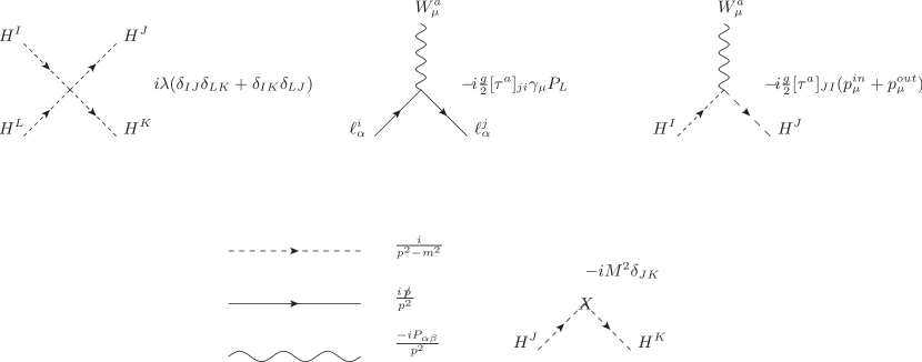
Figure 6: Feynman rules for dimension-four interactions. For the gauge boson propagator $P_{\alpha\beta}=g_{\alpha\beta}+(\xi-1)k_{\alpha}k_{\beta}/k^{2}$.

The Pauli matrices and antisymmetric $\epsilon$ are

$$\epsilon=\left[\begin{array}[]{cc}0&1\\ -1&0\end{array}\right]~{}~{},~{}~{}\vec{\tau}=\left(\left[\begin{array}[]{cc}0&1\\ 1&0\end{array}\right],\left[\begin{array}[]{cc}0&-i\\ i&0\end{array}\right],\left[\begin{array}[]{cc}1&0\\ 0&-1\end{array}\right]\right)~{}~{}~{}.$$ (A.9)

The following identities are useful:

$$2\epsilon_{iI}\epsilon_{jJ} = \delta_{ij}\delta_{IJ}-\tau_{ij}^{a}\tau_{a,IJ}~{}~{}{\rm Fierz}$$ (A.10)

$$\frac{1}{4}\tau_{ij}^{a}\tau_{a,kl} = \frac{1}{2}\delta_{il}\delta_{kj}-\frac{1}{4}\delta_{ij}\delta_{kl}~{}~{}~{}~{}{\rm SU(N)}$$

$$\epsilon_{iJ}\epsilon_{kJ} = \delta_{ik}$$

where the first two imply

$$\epsilon_{ij}\epsilon_{kl} = \delta_{ik}\delta_{jl}-\delta_{il}\delta_{jk}.$$ (A.11)

Appendix B Dimension eight four-fermion operators

B.1 constructing all possible SU(2) contractions

The aim is to build all possible SU(2) contractions for an operator constructed from the fields:

$$(\overline{\ell}^{i}_{\rho}\gamma_{\alpha}\ell^{j}_{\sigma})(\overline{q}^{k}\gamma^{\alpha}q^{l})(H^{\dagger M}H^{N})$$ (B.1)

where $\{i,j,k,l,M,N\}$ are SU(2) indices. For $R$ in the doublet representation of SU(2), invariants can be constructed as follows:

$$R^{\dagger}R~{}~{},~{}~{}R\epsilon R~{}~{},~{}~{}R^{*}\epsilon R^{*}~{}~{},~{}~{}R^{\dagger}\tau^{a}RR^{\dagger}\tau^{a}R~{}~{}~{},~{}~{}\varepsilon_{abc}R^{\dagger}\tau^{a}RR^{\dagger}\tau^{b}RR^{\dagger}\tau^{c}R~{}~{}.$$

Consider first the $\tau\tau\tau$ contraction. Multiplying the product of two Pauli matrices by $\sum_{a,b}\tau^{a}\tau^{b}$ gives:

$$\sum_{a,b}\tau_{ij}^{a}\tau_{kl}^{b}{\Big{(}}\tau^{a}_{MR}\tau^{b}_{RN}{\Big{)}}=\sum_{a,b}\tau_{ij}^{a}\tau_{kl}^{b}{\Big{(}}\delta^{ab}\delta_{MN}+\sum_{c}i\varepsilon^{abc}\tau^{c}_{MN}{\Big{)}}$$ (B.2)

and using the identities of eqn (A.10), allows to write:

$$i\varepsilon^{abc}\tau_{ij}^{a}\tau_{kl}^{b}\tau^{c}_{mn} = 2\delta_{il}\delta_{Mj}\delta_{kN}-\delta_{ij}\delta_{Ml}\delta_{kN}-\delta_{iN}\delta_{kl}\delta_{Mj}-\delta_{il}\delta_{kj}\delta_{MN}+\delta_{ij}\delta_{kl}\delta_{MN}$$ (B.3)

so this operator can be exchanged for $\delta\delta\delta$ contractions. The $\tau\tau$, and $\epsilon\epsilon$ contractions can be rewritten as $\delta\delta$s using the Fierz and SU(2) identities of eqn (A.10), so a complete set of operators is the inequivalent $\delta\delta\delta$ contractions.

There are six possible $\delta\delta\delta$ contractions (the permutations of three objects) for the fields of eqn (B.1):

$$\delta_{ij}\delta_{kl}\delta_{MN} ~{}~{}~{}~{}~{}~{}~{}~{}~{}~{}~{}~{}~{}~{}~{}~{}~{}~{}~{}~{}~{}~{}~{}~{}~{}~{}~{}~{}~{}~{}\to{\cal O}_{S}$$

$$= \delta_{kl}(-\epsilon_{iM}\epsilon_{Nj}+\delta_{kN}\delta_{Ml})\to{\cal O}_{H2}-{\cal O}_{NSI}$$

$$\delta_{il}\delta_{kj}\delta_{MN} = \frac{1}{2}(\delta_{ij}\delta_{kl}+\tau^{a}_{ij}\tau^{a}_{kl})\delta_{MN}\to\frac{1}{2}{\cal O}_{S}+\frac{1}{2}{\cal O}_{TLQ}$$

$$= \frac{1}{2}{\Big{\{}}\delta_{il}(\delta_{kN}\delta_{Mj}-\epsilon_{kM}\epsilon_{Nj})+\delta_{kj}(\delta_{iN}\delta_{Ml}-\epsilon_{iM}\epsilon_{Nl}){\Big{\}}}\to\frac{1}{2}({\cal O}_{CCLFV}+{\cal O}_{CCLFV}^{\dagger}-{\cal O}_{CCNSI}-{\cal O}_{CCNSI}^{\dagger})$$

$$\delta_{iN}\delta_{kl}\delta_{Mj} ~{}~{}~{}~{}~{}~{}~{}~{}~{}~{}~{}~{}~{}~{}~{}~{}~{}~{}~{}~{}~{}~{}~{}~{}~{}~{}~{}~{}~{}~{}\to{\cal O}_{H2}$$

$$= \frac{1}{2}(\delta_{ij}\delta_{MN}+\tau^{a}_{ij}\tau^{a}_{MN})\delta_{kl}\to\frac{1}{2}{\cal O}_{S}+\frac{1}{2}{\cal O}_{TLH}$$

$$\delta_{ij}\delta_{kN}\delta_{Ml} = \frac{1}{2}(\delta_{kl}\delta_{MN}+\tau^{a}_{kl}\tau^{a}_{MN})\delta_{ij}\to\frac{1}{2}{\cal O}_{S}+\frac{1}{2}{\cal O}_{TQH}$$

$$\delta_{il}\delta_{kN}\delta_{Mj} ~{}~{}~{}~{}~{}~{}~{}~{}~{}~{}~{}~{}~{}~{}~{}~{}~{}~{}~{}~{}~{}~{}~{}~{}~{}~{}~{}~{}~{}~{}\to{\cal O}_{CCLFV}$$

$$\delta_{iN}\delta_{kj}\delta_{Ml} ~{}~{}~{}~{}~{}~{}~{}~{}~{}~{}~{}~{}~{}~{}~{}~{}~{}~{}~{}~{}~{}~{}~{}~{}~{}~{}~{}~{}~{}~{}\to{\cal O}_{CCLFV}^{\dagger}$$ (B.4)

where after the arrows, the contractions are related to the bases of BR and of this manuscript. We find one relationship among these contractions:

$$\delta_{ij}\delta_{kl}\delta_{MN}-\delta_{il}\delta_{kj}\delta_{MN}-\delta_{iN}\delta_{kl}\delta_{Mj}-\delta_{ij}\delta_{kN}\delta_{Ml}+\delta_{il}\delta_{kN}\delta_{Mj}+\delta_{iN}\delta_{kj}\delta_{Ml}=0~{}~{}~{},$$ (B.5)

which will be used to remove the fourth contraction of eqn (B.4).

B.2 Alternate bases for SU(2) doublet external fermions

In this manuscript, we use a different basis of dimension eight operators from Berezhiani and Rossi, constructed such that the operators match at tree level onto either NSI, or LFV.

These operators are constructed with doublet first generation quarks $q$ as external fermions; they will also be appropriate (for the lepton flavour indices $\{\rho,\sigma\}\in\{\mu,\tau\}$) when the external fermion is a doublet first generation lepton. The dimension six operators in our basis are given in eqn (II.10), and the dimension eight operators are in eqn (II.11).

Comments on this basis:

1. ${\cal O}_{NSI}$ is the same operator as for singlet external fermions, and can be exchanged for the first contraction of eqn (B.4). It matches at $m_{W}$ onto low-energy NSI.

2. The second contraction of eqn (B.4) is hermitian, so we exchange this $\delta\delta\delta$ contraction for $({\cal O}_{CCNSI}+{\cal O}^{\dagger}_{CCNSI}),$ which will match at $m_{W}$ to NSI and CC operators.

3. Similarly, ${\cal O}_{H2}$ is like for external singlets, matches at $m_{W}$ only onto LFV four-fermion operators, and corresponds to the third contraction of eqn (B.4).

4. the fourth contraction of eqn (B.4) would match onto both NSI and LFV, so we use the identity (B.5) to remove it. It can be written as

   $$(\overline{\ell}_{\rho}\gamma_{\alpha}\ell_{\sigma})(\overline{q}H)\gamma_{\alpha}(H^{\dagger}q) = -{\cal O}_{NSI}+\frac{1}{2}({\cal O}_{CCLFV}+{\cal O}_{CCLFV}^{\dagger})+\frac{1}{2}({\cal O}_{CCNSI}+{\cal O}_{CCNSI}^{\dagger})$$ (B.6)

5. The last two contractions of eqn (B.4) are ${\cal O}_{CCLFV}$ and ${\cal O}_{CCLFV}^{\dagger}$, who match onto Charged Current and LFV operators below $m_{W}$.

   The one-loop RGEs turn out to only involve the combination $C_{CCLFV,q}+C^{\dagger}_{CCLFV,q}$. So in the body of the manuscript, these operators are combined into ${\cal O}_{CCLFV+}=({\cal O}_{CCLFV}+{\cal O}^{\dagger}_{CCLFV})$ . The RGEs are calculated separately for $C_{CCLFV,q}^{\rho\sigma}$, $[C^{\dagger}_{CCLFV,q}]^{\rho\sigma}$, $C_{CCNSI,q}^{\rho\sigma}$, $[C^{\dagger}_{CCNSI,q}]^{\rho\sigma}$, then the coefficient $C_{+}$ of ${\cal O}^{\rho\sigma}_{+}$ can be obtained by setting

   $$C_{+}({\cal O}+{\cal O}^{\dagger})+C_{-}({\cal O}-{\cal O}^{\dagger})=C{\cal O}+C^{\dagger}{\cal O}^{\dagger}\;,$$

   which gives $C_{+}=(C+C^{\dagger})/2$.

Appendix C Matching at $m_{W}$

In this study, we should in principle use the one-loop minimisation condition. This is because the coupling constants of renormalisable interactions run, which should be taken into account in solving the RGEs for the operator coefficients. If one does so, $g,\lambda$ and $\eta$ in the anomalous dimension matrices of eqn(III.8) are scale-dependent and, in the solutions at $\mu_{f}$, should be evaluated at $\mu_{f}$. The minimisation conditions therefore should be expressed in terms of running parameters at $m_{W}$. Then, it is well known (see eg FJJ ), that it is the sum of the tree potential,expressed in terms of running parameters, + the one-loop effective potential, that is independent of the renormalisation scale $\mu$.

However in practise, we often use the tree minimisation conditions, when the RGEs give loop contributions to LFV at the same order as the one-loop matching conditions, because we are only interested in the loop order at which LFV is induced, and not in the precise value of the LFV operator coefficients.

It is convenient to write the one-loop minimisation condition as

$$0 = v\left\{-M^{2}(\mu)\left(1+\frac{1}{\kappa}L_{M2}\right)+v^{2}\left(\lambda(\mu)+\frac{1}{\kappa}L_{H2}\right)\right\}\equiv v(\widetilde{M}^{2}-\widetilde{\lambda}v^{2})\;.$$ (C.1)

Minimising the one-loop effective potential given in FJJ (with $v^{2}_{here}=v^{2}/2|_{FJJ}$, and $\lambda_{here}=\lambda_{FJJ}/3$), and evaluating at $\mu^{2}=m_{W}^{2}$, gives

$$L_{H2} = \frac{9\lambda^{2}}{2}\left(\ln\frac{m_{H}^{2}}{m_{W}^{2}}-\frac{2}{3}\right)-6y_{t}^{4}\left(\ln\frac{m_{t}^{2}}{m_{W}^{2}}-\frac{1}{2}\right)+\frac{g^{4}}{8}+\frac{3(g^{2}+g^{{}^{\prime}2})^{2}}{8}\left(\ln\frac{m_{Z}^{2}}{m_{W}^{2}}+\frac{1}{6}\right)$$ (C.2)

$$L_{M2} = \frac{3\lambda}{2}\left(\ln\frac{m_{H}^{2}}{m_{W}^{2}}-1\right)\;.$$ (C.3)

References

• (1) L. Wolfenstein, “Neutrino Oscillations in Matter,” Phys. Rev. D 17 (1978) 2369. doi:10.1103/PhysRevD.17.2369 J. W. F. Valle, “Resonant Oscillations of Massless Neutrinos in Matter,” Phys. Lett. B 199 (1987) 432. doi:10.1016/0370-2693(87)90947-6 M. M. Guzzo, A. Masiero and S. T. Petcov, “On the MSW effect with massless neutrinos and no mixing in the vacuum,” Phys. Lett. B 260 (1991) 154. doi:10.1016/0370-2693(91)90984-X
• (2) Y. Farzan and M. Tortola, “Neutrino oscillations and Non-Standard Interactions,” Front. in Phys.  6 (2018) 10 [arXiv:1710.09360 [hep-ph]].
• (3) Z. Berezhiani and A. Rossi, “Limits on the nonstandard interactions of neutrinos from e+ e- colliders,” Phys. Lett. B 535 (2002) 207 [hep-ph/0111137].
• (4) S. Davidson, C. Pena-Garay, N. Rius and A. Santamaria, “Present and future bounds on nonstandard neutrino interactions,” JHEP 0303 (2003) 011 doi:10.1088/1126-6708/2003/03/011 [hep-ph/0302093].
• (5) C. Biggio, M. Blennow and E. Fernandez-Martinez, “General bounds on non-standard neutrino interactions,” JHEP 0908 (2009) 090 doi:10.1088/1126-6708/2009/08/090 [arXiv:0907.0097 [hep-ph]].
• (6) P. Coloma, “Non-Standard Interactions in propagation at the Deep Underground Neutrino Experiment,” JHEP 1603 (2016) 016 doi:10.1007/JHEP03(2016)016 [arXiv:1511.06357 [hep-ph]]. S. Choubey, A. Ghosh, T. Ohlsson and D. Tiwari, “Neutrino Physics with Non-Standard Interactions at INO,” JHEP 1512 (2015) 126 doi:10.1007/JHEP12(2015)126 [arXiv:1507.02211 [hep-ph]]. A. de Gouvêa and K. J. Kelly, “Non-standard Neutrino Interactions at DUNE,” Nucl. Phys. B 908 (2016) 318 doi:10.1016/j.nuclphysb.2016.03.013 [arXiv:1511.05562 [hep-ph]]. J. Liao, D. Marfatia and K. Whisnant, “Nonstandard neutrino interactions at DUNE, T2HK and T2HKK,” JHEP 1701 (2017) 071 doi:10.1007/JHEP01(2017)071 [arXiv:1612.01443 [hep-ph]]. S. Fukasawa, M. Ghosh and O. Yasuda, “Sensitivity of the T2HKK experiment to nonstandard interactions,” Phys. Rev. D 95 (2017) no.5, 055005 doi:10.1103/PhysRevD.95.055005 [arXiv:1611.06141 [hep-ph]]. K. Huitu, T. J. Kärkkäinen, J. Maalampi and S. Vihonen, “Constraining the nonstandard interaction parameters in long baseline neutrino experiments,” Phys. Rev. D 93 (2016) no.5, 053016 doi:10.1103/PhysRevD.93.053016 [arXiv:1601.07730 [hep-ph]]. J. Kopp, M. Lindner, T. Ota and J. Sato, “Non-standard neutrino interactions in reactor and superbeam experiments,” Phys. Rev. D 77 (2008) 013007 doi:10.1103/PhysRevD.77.013007 [arXiv:0708.0152 [hep-ph]]. M. Blennow, S. Choubey, T. Ohlsson, D. Pramanik and S. K. Raut, “A combined study of source, detector and matter non-standard neutrino interactions at DUNE,” JHEP 1608 (2016) 090 doi:10.1007/JHEP08(2016)090 [arXiv:1606.08851 [hep-ph]]. M. Masud and P. Mehta, “Nonstandard interactions and resolving the ordering of neutrino masses at DUNE and other long baseline experiments,” Phys. Rev. D 94 (2016) no.5, 053007 doi:10.1103/PhysRevD.94.053007 [arXiv:1606.05662 [hep-ph]]. S. K. Agarwalla, S. S. Chatterjee and A. Palazzo, “Degeneracy between $\theta_{23}$ octant and neutrino non-standard interactions at DUNE,” Phys. Lett. B 762 (2016) 64 doi:10.1016/j.physletb.2016.09.020 [arXiv:1607.01745 [hep-ph]]. K. N. Deepthi, S. Goswami and N. Nath, “Challenges posed by non-standard neutrino interactions in the determination of $\delta_{CP}$ at DUNE,” Nucl. Phys. B 936 (2018) 91 doi:10.1016/j.nuclphysb.2018.09.004 [arXiv:1711.04840 [hep-ph]].
• (7) A. Esmaili and A. Y. Smirnov, “Probing Non-Standard Interaction of Neutrinos with IceCube and DeepCore,” JHEP 1306 (2013) 026 doi:10.1007/JHEP06(2013)026 [arXiv:1304.1042 [hep-ph]]. T. Ohlsson, H. Zhang and S. Zhou, “Effects of nonstandard neutrino interactions at PINGU,” Phys. Rev. D 88 (2013) no.1, 013001 doi:10.1103/PhysRevD.88.013001 [arXiv:1303.6130 [hep-ph]]. S. Fukasawa and O. Yasuda, “Constraints on the Nonstandard Interaction in Propagation from Atmospheric Neutrinos,” Adv. High Energy Phys.  2015 (2015) 820941 doi:10.1155/2015/820941 [arXiv:1503.08056 [hep-ph]]. S. Fukasawa and O. Yasuda, “The possibility to observe the non-standard interaction by the Hyperkamiokande atmospheric neutrino experiment,” Nucl. Phys. B 914 (2017) 99 doi:10.1016/j.nuclphysb.2016.11.004 [arXiv:1608.05897 [hep-ph]]. I. Mocioiu and W. Wright, “Non-standard neutrino interactions in the mu–tau sector,” Nucl. Phys. B 893 (2015) 376 doi:10.1016/j.nuclphysb.2015.02.016 [arXiv:1410.6193 [hep-ph]].
• (8) I. Esteban, M. C. Gonzalez-Garcia, M. Maltoni, I. Martinez-Soler and J. Salvado, “Updated Constraints on Non-Standard Interactions from Global Analysis of Oscillation Data,” JHEP 1808 (2018) 180 doi:10.1007/JHEP08(2018)180 [arXiv:1805.04530 [hep-ph]].
• (9) C. Giunti, “General COHERENT Constraints on Neutrino Non-Standard Interactions,” arXiv:1909.00466 [hep-ph].
• (10) C. J. Stapleford, D. J. Väänänen, J. P. Kneller, G. C. McLaughlin and B. T. Shapiro, “Nonstandard Neutrino Interactions in Supernovae,” Phys. Rev. D 94 (2016) no.9, 093007 doi:10.1103/PhysRevD.94.093007 [arXiv:1605.04903 [hep-ph]]. M. Blennow, A. Mirizzi and P. D. Serpico, “Nonstandard neutrino-neutrino refractive effects in dense neutrino gases,” Phys. Rev. D 78 (2008) 113004 doi:10.1103/PhysRevD.78.113004 [arXiv:0810.2297 [hep-ph]].
• (11) A. Chatelain and M. C. Volpe, “Neutrino propagation in binary neutron star mergers in presence of nonstandard interactions,” Phys. Rev. D 97 (2018) no.2, 023014 doi:10.1103/PhysRevD.97.023014 [arXiv:1710.11518 [hep-ph]].
• (12) P. F. de Salas and S. Pastor, “Relic neutrino decoupling with flavour oscillations revisited,” JCAP 1607 (2016) no.07, 051 doi:10.1088/1475-7516/2016/07/051 [arXiv:1606.06986 [hep-ph]].
• (13) P. D. Serpico, “Standard and non-standard primordial neutrinos,” Phys. Scripta T 127 (2006) 95 doi:10.1088/0031-8949/2006/T127/032 [astro-ph/0606044].
• (14) P. Huber, T. Schwetz and J. W. F. Valle, “Confusing nonstandard neutrino interactions with oscillations at a neutrino factory,” Phys. Rev. D 66 (2002) 013006 doi:10.1103/PhysRevD.66.013006 [hep-ph/0202048].
• (15) D. Aristizabal Sierra, V. De Romeri and N. Rojas, “COHERENT analysis of neutrino generalized interactions,” Phys. Rev. D 98 (2018) 075018 [arXiv:1806.07424 [hep-ph]].
• (16) W. Altmannshofer, M. Tammaro and J. Zupan, “Non-standard neutrino interactions and low energy experiments,” arXiv:1812.02778 [hep-ph].
• (17) A. Falkowski, M. González-Alonso and Z. Tabrizi, “Reactor neutrino oscillations as constraints on Effective Field Theory,” arXiv:1901.04553 [hep-ph].
• (18) I. Bischer and W. Rodejohann, “General Neutrino Interactions from an Effective Field Theory Perspective,” Nucl. Phys. B 947 (2019) 114746 doi:10.1016/j.nuclphysb.2019.114746 [arXiv:1905.08699 [hep-ph]].
• (19) D. Akimov et al. [COHERENT Collaboration], “Observation of Coherent Elastic Neutrino-Nucleus Scattering,” Science 357 (2017) no.6356, 1123 [arXiv:1708.01294 [nucl-ex]]. D. Akimov et al. [COHERENT Collaboration], “COHERENT Collaboration data release from the first observation of coherent elastic neutrino-nucleus scattering,” arXiv:1804.09459 [nucl-ex].
• (20) S. Bergmann, Y. Grossman and E. Nardi, “Neutrino propagation in matter with general interactions,” Phys. Rev. D 60 (1999) 093008 doi:10.1103/PhysRevD.60.093008 [hep-ph/9903517].
• (21) M. Cirelli, E. Del Nobile and P. Panci, “Tools for model-independent bounds in direct dark matter searches,” JCAP 1310 (2013) 019 doi:10.1088/1475-7516/2013/10/019 [arXiv:1307.5955 [hep-ph]].
• (22) V. Cirigliano, S. Davidson and Y. Kuno, “Spin-dependent $\mu\to e$ conversion,” Phys. Lett. B 771 (2017) 242 doi:10.1016/j.physletb.2017.05.053 [arXiv:1703.02057 [hep-ph]].
• (23) B. Grzadkowski, M. Iskrzynski, M. Misiak and J. Rosiek, “Dimension-Six Terms in the Standard Model Lagrangian,” JHEP 1010 (2010) 085 [arXiv:1008.4884 [hep-ph]].
• (24) R. Alonso, E. E. Jenkins, A. V. Manohar and M. Trott, “Renormalization Group Evolution of the Standard Model Dimension Six Operators III: Gauge Coupling Dependence and Phenomenology,” JHEP 1404 (2014) 159 [arXiv:1312.2014 [hep-ph]]. E. E. Jenkins, A. V. Manohar and M. Trott, “Renormalization Group Evolution of the Standard Model Dimension Six Operators II: Yukawa Dependence,” JHEP 1401 (2014) 035 [arXiv:1310.4838 [hep-ph]]. E. E. Jenkins, A. V. Manohar and M. Trott, “Renormalization Group Evolution of the Standard Model Dimension Six Operators I: Formalism and lambda Dependence,” JHEP 1310 (2013) 087 [arXiv:1308.2627 [hep-ph]].
• (25) A. Crivellin, S. Davidson, G. M. Pruna and A. Signer, “Renormalisation-group improved analysis of $\mu\to e$ processes in a systematic effective-field-theory approach,” JHEP 1705 (2017) 117 [arXiv:1702.03020 [hep-ph]].
• (26) K. S. Babu, P. S. B. Dev, S. Jana and A. Thapa, “Non-Standard Interactions in Radiative Neutrino Mass Models,” arXiv:1907.09498 [hep-ph].
• (27) M. B. Gavela, D. Hernandez, T. Ota and W. Winter, “Large gauge invariant non-standard neutrino interactions,” Phys. Rev. D 79 (2009) 013007 [arXiv:0809.3451 [hep-ph]].
• (28) S. Antusch, J. P. Baumann and E. Fernandez-Martinez, “Non-Standard Neutrino Interactions with Matter from Physics Beyond the Standard Model,” Nucl. Phys. B 810 (2009) 369 doi:10.1016/j.nuclphysb.2008.11.018 [arXiv:0807.1003 [hep-ph]].
• (29) M. Pospelov and J. Pradler, “Elastic scattering signals of solar neutrinos with enhanced baryonic currents,” Phys. Rev. D 85 (2012) 113016 Erratum: [Phys. Rev. D 88 (2013) no.3, 039904] doi:10.1103/PhysRevD.85.113016, 10.1103/PhysRevD.88.039904 [arXiv:1203.0545 [hep-ph]].
• (30) Y. Farzan, “A model for large non-standard interactions of neutrinos leading to the LMA-Dark solution,” Phys. Lett. B 748 (2015) 311 doi:10.1016/j.physletb.2015.07.015 [arXiv:1505.06906 [hep-ph]].
• (31) Y. Farzan and J. Heeck, “Neutrinophilic nonstandard interactions,” Phys. Rev. D 94 (2016) no.5, 053010 doi:10.1103/PhysRevD.94.053010 [arXiv:1607.07616 [hep-ph]].
• (32) C. Biggio, M. Blennow and E. Fernandez-Martinez, “Loop bounds on non-standard neutrino interactions,” JHEP 0903 (2009) 139 doi:10.1088/1126-6708/2009/03/139 [arXiv:0902.0607 [hep-ph]].
• (33) U. Bellgardt et al. [SINDRUM Collaboration], “Search for the Decay $\mu^{+}\to e^{+}e^{+}e^{-}$,” Nucl. Phys. B 299 (1988) 1.
• (34) W. H. Bertl et al. [SINDRUM II Collaboration], “A Search for muon to electron conversion in muonic gold,” Eur. Phys. J. C 47 (2006) 337. doi:10.1140/epjc/s2006-02582-x C. Dohmen et al. [SINDRUM II Collaboration], “Test of lepton flavor conservation in $\mu\to e$ conversion on titanium,” Phys. Lett. B 317 (1993) 631. W. Honecker et al. [SINDRUM II Collaboration], “Improved limit on the branching ratio $\mu\to e$ conversion on lead,” Phys. Rev. Lett.  76 (1996) 200. doi:10.1103/PhysRevLett.76.200
• (35) Y. Kuno [COMET Collaboration], “A search for muon-to-electron conversion at J-PARC: The COMET experiment,” PTEP 2013 (2013) 022C01. doi:10.1093/ptep/pts089
• (36) R. M. Carey et al. [Mu2e Collaboration], “Proposal to search for $\mu^{-}N\to e^{-}N$ with a single event sensitivity below $10^{-16}$,” FERMILAB-PROPOSAL-0973.
• (37) A. Blondel et al., “Research Proposal for an Experiment to Search for the Decay $\mu\to eee$,” arXiv:1301.6113 [physics.ins-det].
• (38) S. Davidson, M. Gorbahn and M. Leak, “Majorana neutrino masses in the renormalization group equations for lepton flavor violation,” Phys. Rev. D 98 (2018) no.9, 095014 doi:10.1103/PhysRevD.98.095014 [arXiv:1807.04283 [hep-ph]].
• (39) B. Aubert et al. [BaBar Collaboration], “Search for Lepton Flavor Violating Decays $\tau^{\pm}\to\ell^{\pm}\pi^{0}$, $\ell^{\pm}\eta$, $\ell^{\pm}\eta^{\prime}$,” Phys. Rev. Lett.  98 (2007) 061803 doi:10.1103/PhysRevLett.98.061803 [hep-ex/0610067].
• (40) Y. Miyazaki et al. [Belle Collaboration], “Search for lepton flavor violating tau- decays into l- eta, l- eta-prime and l- pi0,” Phys. Lett. B 648 (2007) 341 doi:10.1016/j.physletb.2007.03.027 [hep-ex/0703009 [HEP-EX]].
• (41) Y. Miyazaki et al. [Belle Collaboration], “Search for Lepton-Flavor-Violating tau Decays into a Lepton and a Vector Meson,” Phys. Lett. B 699 (2011) 251 doi:10.1016/j.physletb.2011.04.011 [arXiv:1101.0755 [hep-ex]].
• (42) D. Black, T. Han, H. J. He and M. Sher, “tau - mu flavor violation as a probe of the scale of new physics,” Phys. Rev. D 66 (2002) 053002 doi:10.1103/PhysRevD.66.053002 [hep-ph/0206056].
• (43) “2017 Review of Particle Physics”, C. Patrignani et al. (Particle Data Group), Chin. Phys. C, 40, 100001 (2016) and 2017 update.
• (44) M. Fujikawa et al. [Belle Collaboration], “High-Statistics Study of the tau- —> pi- pi0 nu(tau) Decay,” Phys. Rev. D 78 (2008) 072006 doi:10.1103/PhysRevD.78.072006 [arXiv:0805.3773 [hep-ex]].
• (45) A. Celis, V. Cirigliano and E. Passemar, “Lepton flavor violation in the Higgs sector and the role of hadronic $\tau$-lepton decays,” Phys. Rev. D 89 (2014) 013008 doi:10.1103/PhysRevD.89.013008 [arXiv:1309.3564 [hep-ph]].
• (46) E. Kou et al. [Belle-II Collaboration], “The Belle II Physics Book,” arXiv:1808.10567 [hep-ex].
• (47) T. Feldmann, “Quark structure of pseudoscalar mesons,” Int. J. Mod. Phys. A 15 (2000) 159 doi:10.1142/S0217751X00000082 [hep-ph/9907491]. H. Leutwyler, “On the 1/N expansion in chiral perturbation theory,” Nucl. Phys. Proc. Suppl.  64 (1998) 223 doi:10.1016/S0920-5632(97)01065-7 [hep-ph/9709408].
• (48) A. M. Baldini et al. [MEG Collaboration], “Search for the lepton flavour violating decay $\mu^{+}\rightarrow e^{+}\gamma$ with the full dataset of the MEG experiment,” Eur. Phys. J. C 76 (2016) no.8, 434 [arXiv:1605.05081 [hep-ex]].
• (49) C. Ford, I. Jack and D. R. T. Jones, “The Standard model effective potential at two loops,” Nucl. Phys. B 387 (1992) 373 Erratum: [Nucl. Phys. B 504 (1997) 551] doi:10.1016/0550-3213(92)90165-8, 10.1016/S0550-3213(97)00532-4 [hep-ph/0111190].