The Lyman Continuum Escape Survey - II: Ionizing Radiation as a Function of the [O iii]$/$[O ii] Line Ratio

Abstract

We discuss the rest-frame optical emission line spectra of a large ($\sim 50$) sample of $z\sim 3.1$ Lyman alpha emitters (LAEs) whose physical properties suggest such sources are promising analogs of galaxies in the reionization era. Reliable Lyman continuum escape fractions have now been determined for a large sample of such LAEs from the Lyman Continuum Escape Survey (LACES) undertaken via deep HST imaging in the SSA22 survey area reported in Fletcher et al. (2019). Using new measures of [O ii] emission secured from Keck MOSFIRE spectra we re-examine, for a larger sample, earlier claims that Lyman continuum leakages may correlate with the nebular emission line ratio [O iii]$/$[O ii] as expected for density-bound Hii regions. We find that a large [O iii]$/$[O ii]  line ratio is indeed a necessary condition for Lyman continuum leakage, strengthening earlier claims made using smaller samples at various redshifts. However, not all LAEs with large [O iii]$/$[O ii] line ratios are leakers and leaking radiation appears not to be associated with differences in other spectral diagnostics. This suggests the detection of leaking radiation is modulated by an additional property, possibly the viewing angle for porous Hii regions. We discuss our new results in the context of the striking bimodality of LAE leakers and non-leakers found in the LACES program and the implications for the sources of cosmic reionization.

1 Introduction

The physical conditions that permit the leakage of ionizing radiation from star-forming galaxies is a topic of great interest. Recent analyses of the demographics and stellar properties of galaxies in the reionization era beyond a redshift $z\simeq 6$ suggest a fraction of $10-20$% of Lyman continuum photons must escape a typical low mass galaxy if such sources govern the process of cosmic reionization (Robertson et al., 2013; Bouwens et al., 2015; Stark, 2016; Dayal & Ferrara, 2018). Since direct measures of Lyman continuum (LyC) leakage are not possible at high redshift due to foreground IGM absorption, most recent work has focused on measures of the LyC escape fraction in low redshift analogs (e.g. Vanzella et al. 2015; Siana et al. 2015; Shapley et al. 2016; Marchi et al. 2017; Rutkowski et al. 2017; Naidu et al. 2018; Steidel et al. 2018; Fletcher et al. 2019).

Lyman alpha emitting galaxies (LAEs) are thought to be the most promising low redshift analogs of sources in the reionization era on account of their low gas-phase metallicity and high star formation rate. Ground-based spectroscopy reveals that many have intense [O iii] emission (Nakajima et al., 2016; Trainor et al., 2016), a property which is inferred indirectly from Spitzer photometry for sources at $z>6$ (Smit et al., 2015; Roberts-Borsani et al., 2016). The Lyman Continuum Escape Survey (LACES) was designed to image a sample of $61$ $z=3.1$ LAEs found using narrow-band Subaru imaging in the SSA22 field (Hayashino et al., 2004; Matsuda et al., 2005; Yamada et al., 2012) using a broad-band F336W filter with the Wide Field Camera 3 (WFC3) onboard Hubble Space Telescope (HST; GO 14747, PI: Robertson). In our first paper in this series (Fletcher et al. 2019, hereafter Paper I), on the basis of spectral energy distribution (SED) fitting, we presented convincing evidence for large escape fractions ($f_{\rm esc}$ $\sim 15-60$%) for individual LAEs for $20$% of the sample, in contrast to strict upper limits for the remainder. We found no strong correlation between this diversity of LyC radiation and other source properties such as stellar mass, UV luminosity and the equivalent widths of [O iii] and Lyman alpha. We speculated on the origin of this curious bimodality in the emergence of ionizing radiation.

The inter-dependence of $f_{\rm esc}$ and nebular line emission was discussed by Nakajima & Ouchi (2014) in terms of their photoionisation models (see also Jaskot & Oey 2013). They found a possible correlation using the emission line ratio [O iii]$/$[O ii] (hereafter O32) which was interpreted in terms of ‘density-bound’ Hii regions. In contrast with ‘ionization-bound’ Hii regions where LyC photons are fully absorbed within the radius of the Stromgren sphere, unusually high values of O32 would reflect partially-incomplete Hii regions where some LyC photons could escape. In this respect, therefore, LAEs would be powerful sources capable of driving cosmic reionization (see also Marchi et al. 2018). At the time of submission of Paper I, a high fraction of the $61$ LACES sources had coverage of [O iii] emission from several Keck MOSFIRE campaigns (Nakajima et al., 2016) but the coverage of [O ii] was limited. Accordingly, we have secured new MOSFIRE data improving the coverage of [O ii] emission across the LACES sample so we can test for the expected trend between O32 and $f_{\rm esc}$ predicted by Nakajima & Ouchi (2014).

A plan of the paper follows. In §2 we discuss the new spectroscopic data, its reduction and estimates of [O ii] emission and hence the O32 ratio. In §3 we revisit the LACES correlations in the context of our new line ratios as well as the strength of the ionizing radiation field. We discuss the results in the context of the bimodality of LyC leakage found in Paper I in §4. Throughout the paper we adopt a concordance cosmology with $\Omega_{\Lambda}$=0.7, $\Omega_{M}$=0.3 and $H_{0}$=70 kms sec^-1 Mpc^-1.

2 Data

2.1 MOSFIRE Observations and Data reduction

Early MOSFIRE observations undertaken in the LACES area were described in Nakajima et al. (2016) and Paper I. As a pilot observation, Nakajima et al. (2016) discuss data for one MOSFIRE pointing (referred to here as mask 1), spectroscopically covered in the K-band (sampling [O iii] and H$\beta$) and the H-band (sampling [O ii] and [Ne iii]). HST/F336W coverage of LACES was determined in part based on this pilot observation. In Paper I, additional K-band spectroscopy for three further MOSFIRE pointings was presented (masks 2–4), one of which (mask 2) was also sampled in the H-band. These additional pointings were chosen to include as many LACES sources as possible with minimal overlap with mask 1. Mask 4 covered almost the same area as mask 2, and was designed primarily to increase the depth for those sources whose K-band spectra were of low signal/noise.

In this paper we present MOSFIRE data from a further pointing (mask 5) undertaken via a long integration in the H-band with the specific goal of improving the coverage of [O ii] emission for sources well-studied in the K-band (i.e. [O iii]) in masks 2–4. The new H-band observations were taken in two second-half nights on UT August 3 and 4 2018 in clear conditions with a seeing of 0.4–0.8 arcsec. Observations were conducted in a similar manner to those reported earlier, adopting a slit width of 0.7 arcsec and individual exposure times of 120 sec with an AB nod sequence of 3 arcsec separation. The total integration time for mask 5 was $4.6$ hr. Table 1 provides a summary of our near-infrared spectroscopic campaign of the LACES sample.

Data reduction was performed using the MOSFIRE DRP in the manner described in Nakajima et al. (2016). All spectroscopic data listed in Table 1 were re-reduced with the latest (2018) version of MOSFIRE DRP. Briefly, the processing includes flat fielding, wavelength calibration, background subtraction and combining the nod positions. Wavelength calibration in the H-band was performed using OH sky lines and in the K-band via a combination of OH lines and Neon arcs. Flux calibration and telluric absorption corrections were obtained from A0V Hipparcos stars observed on the same night under the same seeing conditions, at similar air masses adopting the same slit width. This procedure corrects for slit losses since most of our LAEs were confirmed with HST images to be unresolved in our ground-based conditions. The cross-calibration between the H- and K-band was independently checked and confirmed with bright stars ($K_{Vega}=15.5$–$16.5$) included on each mask. Some Lyman-break galaxies (LBGs) that were also placed on the masks for a comparison sample are more extended than LAEs in the HST image, and their slit losses would not be fully corrected for with the above method. We quantified the potential additional slit losses for the LBGs by using an appropriately smoothed HST image using the seeing and slit position/angles appropriate for the observations. We find for the small subset of LBG targets, the additional flux losses would be smaller than 25%. This is minimal and does not affect our conclusions.

Table 1: MOSFIRE Near-Infrared Spectroscopy of the LACES Sample

Name	Band	Date	Seeing	Exp.	$N^{o}$	Ref.
				(hrs)	(1)	(2)
mask1	K	2015 Jun 20	$0\farcs 4$–$0\farcs 5$	3.0	17	(a)
	H	2015 Jun 21	$0\farcs 4$–$0\farcs 5$	2.5	17	(a)
mask2	K	2017 Jul 31	$0\farcs 6$–$0\farcs 9$	3.0	21	(b)
	H	2017 Aug 1	$0\farcs 5$–$0\farcs 9$	3.1	21	(b)
mask3	K	2017 Aug 1	$0\farcs 5$–$0\farcs 8$	2.3	17	(b)
mask4	K	2017 Aug 1	$0\farcs 3$–$0\farcs 5$	2.0	19	(b)
mask5	H	2018 Aug 3, 4	$0\farcs 4$–$0\farcs 8$	4.6	21	(c)
Full (†)	K			2.0–6.0	53	(c)
	H			2.5–10.2	38	(c)

Note. — (1) Number of targeted LACES sources. (2) Relevant campaigns (a) Nakajima et al. (2016); (b) Paper I; (c) This work. (${\dagger}$) Full sample in K and H taking into account multiply-observed spectra.

The resulting K-band observations span four different masks, including $18$ objects that were observed on more than one mask. For each of these multiply-observed sources, we combined flux-calibrated 2D spectra from different masks to generate a final 2D spectrum after the spatial zero points were aligned. Our final K-band spectroscopic sample contains $53$ LACES sources each with a total integration time ranging from 2.0 to 6.0 hrs. Similarly, we have H-band coverage of $38$ LACES sources with integration times ranging from $2.5$–$10.2$ hrs. All H-band sources have K-band coverage. We experimented with coaddition of the various integrations using both 2D spectra from which 1D spectra were subsequently extracted, as well as summation of 1D spectra individually extracted; no significant difference in S/N was found.

One dimensional (1D) spectra were produced via the summation of 5–9 pixels along the spatial direction centered on the expected spatial position. This width was chosen to maximize the signal-to-noise (S/N) ratio and corresponds approximately to twice the average seeing for the observations.

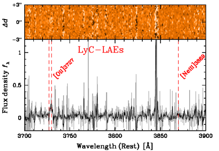
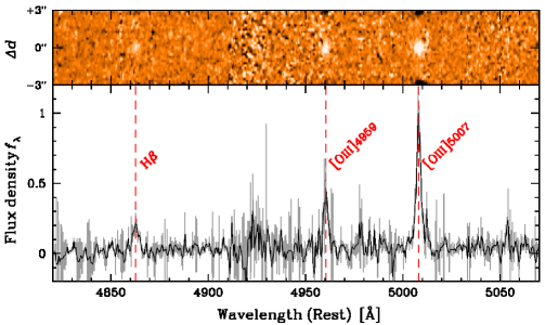
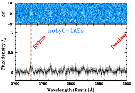
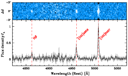
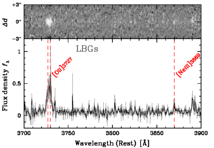
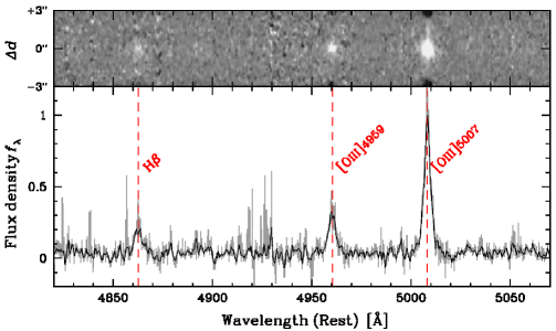
Figure 1: Composite rest-frame optical spectra of LAEs with a significant HST LyC detection (LyC-LAEs; top), LAEs with no detectable LyC flux (noLyC-LAEs; middle), and LBGs (all undetected in LyC; bottom). These spectra were generated with the [O iii]-normalized individual spectra for measuring line flux ratios (see text for more details). The grey shaded region around each spectrum refers to the standard deviation of the flux density at each wavelength estimated by bootstrap resampling (see the text for details). The wavelengths of key diagnostic emission lines are marked with a red dashed line.

2.2 Emission line identifications

Out of the $53$ K-band sources, $38$ have confirmed Ly$\alpha$ emission from our earlier optical campaigns (see Nakajima et al. (2018a) for details). For the other LAEs, their redshifts are fairly well-constrained from the Subaru narrowband filter used for the selection. Using these redshifts as an initial guess, we visually examined the 1D and 2D spectra for detectable [O iii]$\lambda\lambda 5007,4959$ and H$\beta$ emission. One or both of [O iii] and H$\beta$ were detected in the MOSFIRE K-band data for $43$ of the $53$ K-band sources and their line fluxes were measured. We then proceeded to measure fluxes for the [O ii] doublet and [Ne iii] emission in the cases where H-band spectra are available ($31$ out of the $43$ with line emission in the K-band). All H-band line fluxes were measured by fitting a Gaussian profile using the IRAF task specfit adopting the redshift and FWHM of the [O iii]$\lambda 5007$. A constant continuum was also considered for each of the [O iii]$+$H$\beta$ and [O ii]+[Ne iii] lines in accounting for background residuals.

To estimate the sky noise level and hence the flux uncertainties, we used more than 1000 apertures with a size equal to that adopted for the flux measurements spread randomly around the emission lines in the 2D spectrum after masking pixels heavily contaminated by OH lines. We then derived the $1\sigma$ fluctuation for each of the lines according to the distribution of the photon counts measured with the randomly distributed apertures. Table 2 lists the measured fluxes and their $1\sigma$ errors for the $43$ identified objects. Among these identified sources, there are $26$, $12$, and $12$ objects whose H$\beta$, [O ii], and [Ne iii] can be individually detected, respectively.

For the $10$ remaining sources with MOSFIRE spectra, three have a spectroscopic redshift based on Ly$\alpha$, where [O iii]$\lambda 5007$ cannot reliably be detected due to a strong OH line . For the other seven targets, without a redshift we cannot determine the expected wavelength of [O iii]$\lambda 5007$ or any other lines and hence upper limits on their fluxes. We therefore exclude these $10$ sources in the following discussion.

Paper I presented $12$ individual LAEs with prominent escape fractions; $f_{\rm esc}$ $\sim 15-60$%. Out of these $12$ $f_{\rm esc}$-detected sources , $11$ ($9$) have K$+$H (only $K$) band MOSFIRE spectra from which $8$ present one or more rest-frame optical emission lines as listed in Table 2. These $8$ sources also have Ly$\alpha$ detections. The remaining $4$ prominent leakers have neither Ly$\alpha$ nor rest-frame optical emission lines; that is they lie in the subsample of $10$ sources discussed above and will not be considered further in this paper.

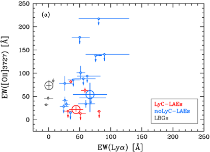
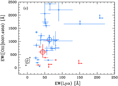
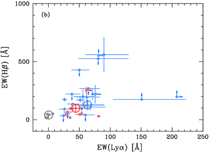
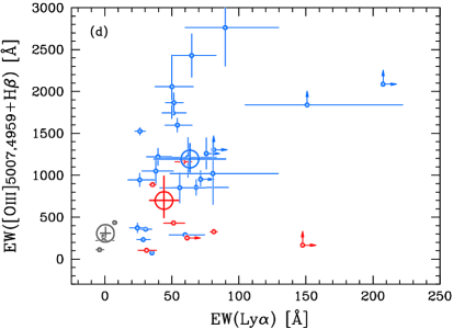
Figure 2: Rest-frame equivalent widths (EWs) of (a) [O ii], (b) H$\beta$, (c) [O iii] and (d) [O iii]$+$H$\beta$ for the three LACES sub-samples (LyC-LAEs in red, noLyC-LAEs in blue, and LBGs in gray) as a function of EW(Ly$\alpha$). Large symbols represent results from stacked spectra whereas the small faint-colored circles shows individual measurements with 3$\sigma$ upper limits shown as arrows.

Table 2: Optical Emission Line Fluxes

Obj.	[O ii]	[Ne iii]	H$\beta$	[O iii]	[O iii]
	doublet	$\lambda 3869$		$\lambda 4959$	$\lambda 5007$
M38	$8.5\pm 0.3$	$1.9\pm 0.2$	$5.3\pm 0.1$	$6.8\pm 0.1$	$20.5\pm 0.1$
2132	$7.6\pm 0.5$	$1.4\pm 0.2$	$2.8\pm 0.3$	$5.9\pm 0.3$	$15.3\pm 0.3$
104037${}^{({\dagger}\,S)}$	$3.6\pm 0.1$	$1.4\pm 0.1$	$2.6\pm 0.1$	$6.9\pm 0.1$	$14.5\pm 0.1$
93564${}^{({\dagger}\,G)}$	$1.8\pm 0.2$	$0.4\pm 0.1$	$2.1\pm 0.2$	$5.2\pm 0.3$	$13.2\pm 0.3$
104511	$0.9\pm 0.2$	$0.9\pm 0.1$	$2.2\pm 0.2$	$5.2\pm 0.1$	$12.0\pm 0.1$
108679	–	–	$<0.8$	$3.5\pm 0.3$	$10.6\pm 0.3$
96688	$4.1\pm 0.3$	$1.7\pm 0.2$	$1.1\pm 0.2$	$3.1\pm 0.2$	$10.0\pm 0.2$
99330	$1.0\pm 0.1$	$0.5\pm 0.1$	$1.1\pm 0.1$	$2.6\pm 0.1$	$8.0\pm 0.1$
109140	–	–	$<0.9$	$2.1\pm 0.2$	$5.8\pm 0.2$
86861${}^{({\dagger}\,G)}$⋆	$<0.7$	$0.9\pm 0.2$	$0.7\pm 0.0$	$1.7\pm 0.2$	$5.4\pm 0.2$
97030	$0.9\pm 0.2$	$0.4\pm 0.1$	$0.7\pm 0.1$	$1.7\pm 0.1$	$4.7\pm 0.1$
92017	–	–	$<0.8$	$0.8\pm 0.2$	$4.0\pm 0.2$
106500	$<0.5$	$0.5\pm 0.1$	$1.2\pm 0.1$	$1.2\pm 0.2$	$3.5\pm 0.2$
104097	$1.8\pm 0.1$	$<0.3$	$1.2\pm 0.1$	$1.0\pm 0.1$	$3.1\pm 0.1$
102334	–	–	$0.7\pm 0.2$	$1.0\pm 0.2$	$2.9\pm 0.2$
94460${}^{({\dagger}\,S)}$	$<0.2$	$<0.2$	$0.4\pm 0.1$	$0.9\pm 0.1$	$2.8\pm 0.1$
102826	$2.0\pm 0.1$	$<0.3$	$0.7\pm 0.1$	$<0.3$	$2.8\pm 0.1$
107585	$<0.4$	$<0.6$	$1.0\pm 0.2$	$0.8\pm 0.2$	$2.3\pm 0.2$
110896	–	–	$<0.7$	$<0.7$	$2.3\pm 0.2$
89114	$<0.4$	$<0.4$	$<0.3$	$0.8\pm 0.1$	$2.3\pm 0.1$
99415	$<0.4$	$<0.3$	$0.5\pm 0.1$	$0.5\pm 0.1$	$1.9\pm 0.1$
97081	$<0.2$	$<0.2$	$0.3\pm 0.1$	$0.6\pm 0.1$	$1.9\pm 0.1$
90428	–	–	$<0.4$	$<1.0$	$1.7\pm 0.3$
93474	$<0.3$	$<0.4$	$<0.5$	$0.6\pm 0.1$	$1.7\pm 0.1$
85165	$<1.0$	$<1.6$	$0.8\pm 0.2$	$0.8\pm 0.2$	$1.6\pm 0.2$
92616${}^{({\dagger}\,G)}$	–	–	$<0.3$	$<0.4$	$1.5\pm 0.1$
104147	$<0.2$	$0.2\pm 0.1$	$<0.2$	$0.2\pm 0.1$	$1.4\pm 0.1$
92219	$<0.3$	$<0.3$	$<0.3$	$<0.2$	$1.4\pm 0.1$
93004	–	–	$<0.4$	$0.7\pm 0.1$	$1.4\pm 0.1$
92235	$0.5\pm 0.1$	$<0.3$	$0.4\pm 0.1$	$<0.4$	$1.4\pm 0.1$
97254	$<0.2$	$<0.2$	$0.3\pm 0.1$	$0.8\pm 0.1$	$1.3\pm 0.1$
97176	$0.3\pm 0.1$	$0.3\pm 0.1$	$<0.2$	$0.4\pm 0.1$	$1.3\pm 0.1$
103371	$<0.2$	$<0.2$	$0.2\pm 0.1$	$0.9\pm 0.1$	$1.3\pm 0.1$
89723	$<0.2$	$<0.2$	$<0.2$	$0.5\pm 0.1$	$1.3\pm 0.1$
110290	$<0.3$	$<0.3$	$0.4\pm 0.1$	$<0.6$	$1.1\pm 0.2$
93981	–	–	$0.4\pm 0.1$	$0.4\pm 0.1$	$1.1\pm 0.1$
105937${}^{({\dagger}\,S)}$	$<0.4$	$<0.3$	$<0.9$	$0.4\pm 0.1$	$1.0\pm 0.1$
91055	$<0.3$	$<0.2$	$0.3\pm 0.1$	$0.3\pm 0.1$	$0.9\pm 0.1$
107677	–	–	$<1.0$	$<0.5$	$0.9\pm 0.2$
95217	$<0.4$	$<0.2$	$<0.6$	$<0.4$	$0.8\pm 0.1$
97128	–	–	$0.7\pm 0.2$	$<0.5$	$0.7\pm 0.2$
101846${}^{({\dagger}\,S)}$	$<0.3$	$<0.3$	$<0.3$	$<0.3$	$0.4\pm 0.1$
90675${}^{({\dagger}\,G)}$¶	–	–	$2.0\pm 0.2$	$<0.5$	$<0.5$

Note. — Fluxes and their $1\sigma$ errors are given in units of $10^{-17}$ erg s^-1 cm^-2. Upper-limits represent the $3\sigma$ values. (${\dagger}$) LyC leaking candidates from Paper I. The $G$ and $S$ denotes the Gold and Silver sample, respectively. ($\star$) The single LAE-AGN in the LACES sample. ($\mathparagraph$) This LAE is likely an extremely metal-poor galaxy on account of its low [O iii]$/$H$\beta$, large H$\beta$ and Ly$\alpha$ EWs, and high $\xi_{\rm ion}$ (see also Table 4).

Table 3: Subsamples of the LACES MOSFIRE campaign

Subsample	for line ratios	for EWs in K/H	for $\xi_{\rm ion}$
LyC-LAEs(†)	$5$	$5$/$5$	$6$
noLyC-LAEs	$20$	$24$/$17$	$29$
LBGs	$5$	$5$/$5$	$6$

Note. — (${\dagger}$) A single AGN-LAE, AGN86861, whose LyC radiation was identified in Paper I has been removed for the stacking analysis and is not counted here.

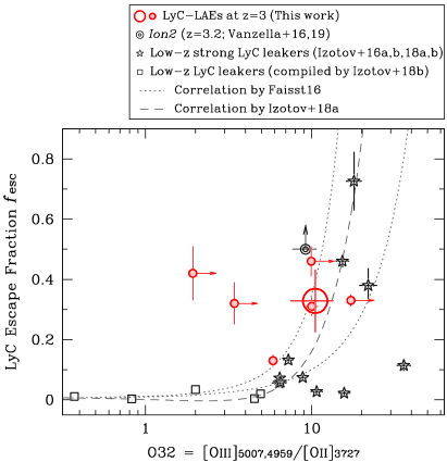
Figure 3: The O32 line ratio vs. escape fraction $f_{\rm esc}$ for the sources with a LyC detection. The large circle represents the LyC-LAEs subsample composite. Other symbols and curves represent literature measures and relations, respectively, as indicated by the legend. The correlation suggests that a prerequisite for a high $f_{\rm esc}$ is a large O32 value.

2.3 Stacked spectra

Despite our significant integration times, we only directly detect individual [O ii] emission lines in a subset of our data (Section 2.2, Table 2). To exploit the full diagnostic value of the rest-frame optical emission lines, we therefore developed a stacking procedure for various subsamples of the LACES catalog. Our goal is to use the stacked spectra to derive average line strengths, line ratios and measures of the ionizing radiation field $\xi_{\rm ion}$ (see §3.2 for definition and more details) and to correlate these properties with the strength of LyC leakage as determined in Paper I.

Accordingly, we divided our spectroscopic sample into three subsamples: LAEs with a clear LyC detection defined as a $>4\sigma$ detection in Paper I (hereafter called “LyC-LAEs” subsample), those LAEs without a clear LyC signal (“noLyC-LAEs” subsample), and LBGs, none of which reveals a LyC signal (“LBGs” subsample). To distinguish LAEs from LBGs we adopted a rest-frame equivalent width (EW) of $20$ Å, derived spectroscopically and/or photometrically, as the demarcation level. The LyC-LAEs subsample includes both the Gold and Silver subsamples in Paper I but excludes the non-thermal source AGN86861. The numbers of sources in each of the subsamples are given in Table 3.

It is important to note that the individual spectra must be normalized in a different manner prior to stacking depending on the physical quantity we seek to measure. For individual line ratios, we use the [O iii] line flux, whereas for EWs and the $\xi_{\rm ion}$ parameter we use the rest-frame optical and UV continuum, respectively, derived from the HST/F160W and the Subaru optical photometry. Naturally for line ratios, we require both H- and K-band spectra, whereas for individual measures of H$\beta$ or [O iii] only K-band data is required. Thus the numbers of useful spectra for stacking varies according to the physical quantity concerned. The details are given in Table 3.

We adopted a stacking procedure very similar to that described in Nakajima et al. (2018a). Briefly, using the individual flux-calibrated spectra in K (H), we shifted each to its rest-frame and rebinned the spectrum to a common dispersion of 0.55 (0.40) Å per pixel. The spectra were then median-stacked with the appropriate normalization as explained above. To exclude positive and negative sky subtraction residuals, we rejected an equal number of the highest and lowest outliers at each pixel corresponding in total to $\simeq 5$ percent of the data. Using an averaging method led to spectra almost indistinguishable from using the median.

To evaluate sample variance and statistical noise, we adopted a bootstrap technique similar to that described in Nakajima et al. (2018a). We generated $1000$ fake composite spectra from the chosen sample. Each fake spectrum was constructed in the same way, using the same number of spectra as the actual composite, but with the list of input spectra formulated by selecting spectra at random, with replacement, from the full list. With these $1000$ fake spectra, we derived the standard deviation at each spectral pixel. The standard deviations are taken into account in calculating the uncertainties of each line flux.

The composite spectra for the three subsamples normalized by their [O iii] fluxes are shown in Figure 1. It is evident that all the key diagnostic emission lines are significantly identified. The difference between the stacked spectra of LAEs and LBGs is immediately apparent e.g. in the [O iii]$/$[O ii] and [Ne iii]$/$[O ii] line ratios.

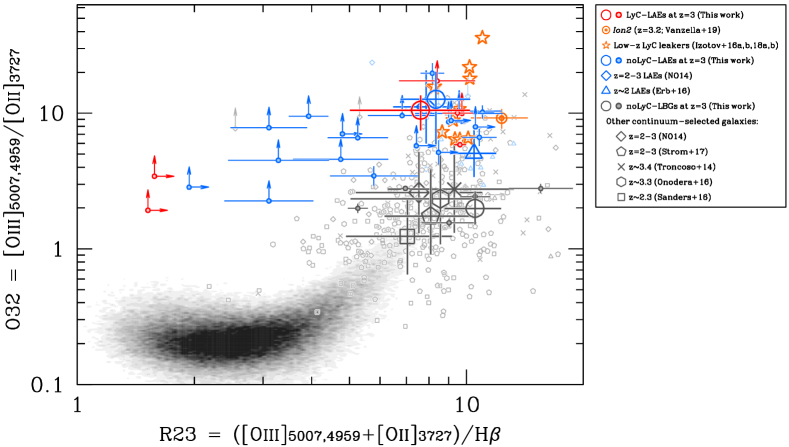
Figure 4: O32 vs. R23 diagram for the LACES and other samples. The LACES subsamples are shown with the same symbols and the colors as in Figure 2. Orange symbols show known LyC leakers, and blue and grey symbols high-$z$ LAEs and continuum-selected galaxies, respectively, compiled from the literature as shown by the legend. If O32 is provided without a [O iii]$\lambda 4959$ contribution, we correct for it assuming the theoretical [O iii]$\lambda 5007/4959$ line ratio of $2.98$ (Storey & Zeippen, 2000). Arrows provide $3\sigma$ lower limits. Grey shading illustrates the equivalent distribution for nearby SDSS galaxies.

2.4 Dust correction to the nebular spectra

Prior to quantitative analysis, it is necessary to consider corrections for dust reddening, particularly for line flux ratios and the $\xi_{\rm ion}$ parameter. Since multiple Balmer emission lines cannot be reliably identified in the individual spectra, the amount of reddening must be estimated using the stellar continuum, assuming that nebular emission and the stellar continuum suffer similar attenuation. Although this assumption remains open to debate at high-$z$, it appears reasonable for young, low-mass star-forming galaxies appropriate for our sample (SFR $\sim 1$–$10$$M_{\odot}$ yr^-1 and M${}_{\star}\sim 10^{8.5}$–$10^{9.5}$$M_{\odot}$; e.g. Reddy et al. 2015).

Earlier studies have tended to indicate LAEs are largely dust-free systems (e.g. Erb et al. 2016; Trainor et al. 2016). Using the SMC extinction curve (Gordon et al., 2003) and the BPASS SEDs, Paper I conducted SED model fitting to constrain the stellar population parameters as well as the amount of dust attenuating the stellar continuum emission. That analysis returned an almost negligible dust attenuation for LAEs irrespective of LyC identification with E(B$-$V) $\simeq 0.01$. Such a small amount of dust is also discussed and supported by our pilot observations in Nakajima et al. (2016), where small Balmer decrements for two bright LAEs were shown to be consistent with zero reddening. Furthermore, Tang et al. (2019) illustrate a monotonic decrease of nebular attenuation with increasing EW of [O iii], showing that the most extreme line emitters with EW([O iii]) $\gtrsim 800$ Å have almost no dust attenuation effect on the nebular emission lines. The relationship derived in Tang et al. (2019) supports the assumption of little dust correction for the LAE sample, given their extremely strong [O iii] emission in general (§3). A similar implication is also drawn in Erb et al. (2016) using the O32 line ratio. A larger value of E(B$-$V) $\simeq 0.10$ was inferred on average for the LBG subsample following the same SED fitting procedure.

Because the E(B$-$V) value is generally uncertain for individual faint sources, we adopt the average of E(B$-$V) $=0.01$ for all the individual and composite spectra for the LAE subsamples, and E(B$-$V) $=0.10$ for the LBGs subsample in the following analysis.

3 Analysis

3.1 Emission lines as a function of $f_{\rm esc}$

We now discuss the correlation between the LyC detections presented in Paper I and both the individual and stacked line measurements derived for the various subsamples of our MOSFIRE spectra. We begin with individual line measures updating and extending some of the results presented in Paper I.

Figure 2 shows that LAEs on average present an intense [O iii] emission line with a rest-frame EW of $\simeq 600-1100$ Å , consistent with the results of our pilot MOSFIRE program (Nakajima et al., 2016). Our enlarged spectroscopic data also reveals more intense H$\beta$ emission with an EW of $>100$ Å . A combined EW of [O iii]$+$H$\beta$ of $\simeq 700-1200$ Å confirms the suggestion that such intermediate redshift LAEs are close analogs of galaxies in the reionization era where the similarly large EWs have been inferred from Spitzer photometry (e.g. Smit et al. 2015; Roberts-Borsani et al. 2016; see also Tang et al. 2019; Reddy et al. 2018).

One of the most interesting questions we can now consider is, via our various spectroscopic measures, what is the physical origin of the bimodal nature of LyC emission seen in the LACES sample (Paper I). In Paper I, we presented a preliminary EW([O iii]) distribution that revealed no significant difference between those LAEs with and without a LyC detection. We can see this is also the case in Figure 2 and the conclusion would not be changed after correcting by a ($1-$$f_{\rm esc}$) factor in order to compensate for escaping (i.e. unconsumed) numbers of ionizing photons.

However, when we turn to consideration of the [O iii]$/$[O ii] ratio which we could not consider in Paper I, a more interesting result emerges. This ratio represents the degree of ionization in the hot ISM and, using photoionization models, Nakajima & Ouchi (2014) argued that intense high ionization lines, e.g. [O iii], and weaker low ionization lines, e.g. [O ii], could arise from density-bounded Hii regions. The associated porosity of the star-forming regions to ionizing radiation would lead to a high $f_{\rm esc}$ (see also Jaskot & Oey 2013; Zackrisson et al. 2013; Behrens et al. 2014).

Figure 3 presents the relationship between $f_{\rm esc}$ and [O iii]$/$[O ii] line ratio for the LACES LyC-LAEs subsample. Our stacked LyC subsample with an average escape fraction $f_{\rm esc}$ $\sim 0.35$ has a large [O iii]$/$[O ii] line ratio of $\simeq 10$. Combining this measurement with individual LyC leaking sources at low-$z$ (Izotov et al., 2016a, b, 2018a, 2018b) as well as a single $z=3$ LyC emitter, Ion2 (Vanzella et al., 2016; de Barros et al., 2016; Vanzella et al., 2019), strengthens the positive correlation presented by Izotov et al. (2018a) and Faisst (2016). Figure 3 shows that a large [O iii]$/$[O ii] ratio is a necessary condition for sources with a high $f_{\rm esc}$. Significantly, the high escape fraction inferred ($f_{\rm esc}$ $>0.1$) is approximately the lower limit necessary if star-forming galaxies govern the reionization process (e.g. Robertson et al. 2015). In our sample, these are only found if the [O iii]$/$[O ii] ratio exceeds $\sim 6-7$.

On the other hand, a large [O iii]$/$[O ii] line ratio need not in every case imply a prominent LyC flux as can be inferred also from the composite spectrum of the noLyC-LAEs (middle panel in Figure 1). This contradiction is also apparent in low-redshift green pea galaxies (Izotov et al., 2018b; Jaskot et al., 2019). We evaluate this further in Figure 4, where we compare our LAEs with and without a LyC detection in the [O iii]$/$[O ii] line ratio versus R23-index diagnostic diagram. This diagram is widely used to examine the gas-phase metallicity and ionization state in the local universe (e.g. Kewley & Dopita 2002) as well as at $z=2-4$ (e.g. Maiolino et al. 2008; Nakajima & Ouchi 2014; Shapley et al. 2015; Onodera et al. 2016; Strom et al. 2017; Sanders et al. 2019). A relatively large scatter in the R23-index at fixed [O iii]$/$[O ii] is seen although for those sources the [O iii]$/$[O ii] measure is only a lower limit (Table 2). This may reflect a low metallicity tail to the distribution for which much larger [O iii]$/$[O ii]  indices are implied. Following Nakajima & Ouchi (2014), Izotov et al. (2016a, b), and Nakajima et al. (2016), we can argue that LAEs and low-$z$ LyC-confirmed green pea galaxies share the similarity in the line emission properties. This work can additionally deduce that both LyC-detected and non-detected LAEs share similar high [O iii]$/$[O ii] line ratios (see also Erb et al. 2016). Such large ratios, indicative of a high ionization parameter are not characteristic of continuum-selected sample at a similar redshift (Troncoso et al., 2014; Onodera et al., 2016; Sanders et al., 2016; Strom et al., 2017) as is confirmed by our own LBG subsample.

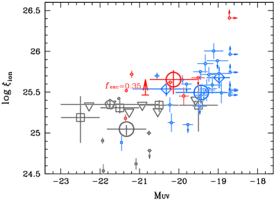
Figure 5: Ionizing photon production efficiency $\xi_{\rm ion}$ as a function of UV absolute magnitude. The symbols and colors for the LACES subsamples are as shown in Figure 2. Large symbols representing average $\xi_{\rm ion}$ values are derived from the stacked spectra (Section 2.3). The individual and the stacked $\xi_{\rm ion}$ are all dust-corrected as detailed in Section 2.4. The red upward-arrow indicates the average degree of correction from $\xi_{\rm ion,0}$ to $\xi_{\rm ion}$for the LyC-LAEs. Blue open diamonds present $\xi_{\rm ion}$ measurements for LAEs at $z=3$ (Nakajima et al., 2018a), and grey open symbols refer to $\xi_{\rm ion}$ measurements for continuum-selected galaxies at $z\simeq 2-4$ (squares from Bouwens et al. 2016, inverse triangles from Shivaei et al. 2018, pentagon from Nakajima et al. 2018b).

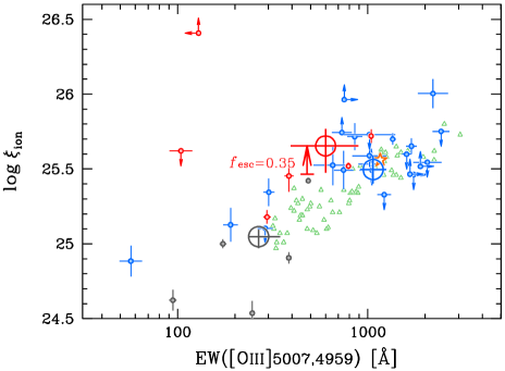
Figure 6: Relationship of [O iii]$/$[O ii] ratio (O32; Left) and ionizing photon production efficiency ($\xi_{\rm ion}$; Right) as a function of EW([O iii]). The LACES sources are plotted with circles as shown in Figure 2. Green triangles present individual (small) and composite (large) measurements of extreme emission line galaxies (EELGs) at $z=1.3-2.4$ (Tang et al., 2019). Orange star illustrates a low-$z$ strong LyC emitting galaxy, J1154+2334, with $f_{\rm esc}$ $=0.46$ (Izotov et al., 2018a; Schaerer et al., 2018). In the left panel, grey open squares show the O32 vs. EW([O iii]) relationship derived with the composites of $z\sim 2.3$ continuum-selected galaxies from MOSDEF (Sanders et al., 2019). If O32 and/or EW([O iii]) is provided without a [O iii]$\lambda 4959$ contribution, we correct for it assuming the theoretical [O iii]$\lambda 5007/4959$ line ratio of $2.98$ (Storey & Zeippen, 2000).

3.2 Ionizing Radiation Field

We finally consider the hardness of the ionizing radiation field which is a further quantity related to the escaping radiation. The efficiency of ionizing photon production is conventionally parameterized by $\xi_{\rm ion}$ defined as:

$$\xi_{\rm ion,0}=\frac{Q_{{\rm H}^{0}}}{L_{\rm UV}}.$$ (1)

The number of ionizing photons, $Q_{{\rm H}^{0}}$, can be determined via hydrogen recombination lines H$\beta$ (e.g Leitherer & Heckman 1995), and the UV luminosity, $L_{\rm UV}$, is derived from the Subaru photometry (Paper I). The subscript $0$ in $\xi_{\rm ion,0}$ indicates that the escape fraction of ionizing photons in this relation is assumed to be zero. The measurable quantity $\xi_{\rm ion}$ can then be derived by dividing $\xi_{\rm ion,0}$ by $(1-f_{\rm esc})$. Our pilot MOSFIRE program together with a rest-frame UV spectroscopic campaign conducted with VIMOS on the VLT indicated that LAEs have $\xi_{\rm ion}$ values significantly larger than those for continuum-selected LBGs (Nakajima et al. 2016, 2018a; see also Matthee et al. 2017).

Figure 5 provides the distribution of $\xi_{\rm ion}$ for the various LACES subsamples. For the LyC-LAEs subsample we adopted an average escape fraction of $f_{esc}$=0.35 to make the conversion. By improving the detectability of H$\beta$ through our recent MOSFIRE campaign, we can confirm our earlier suggestion that $\xi_{\rm ion}$ is significantly larger for LAEs than for continuum-selected LBGs. But again, we can see that both LyC-detected and non-detected LAEs subsamples have comparable values, $\log$ $\xi_{\rm ion}$ $\simeq 25.5-25.7$, providing further evidence that the two populations of LAEs are spectroscopically indistinguishable. LAEs with LyC leakage are more efficient producers of ionizing photons at a given UV luminosity by $\simeq 0.3-0.4$ dex compared to continuum-selected LBGs but by only $\simeq 0.1$ dex with respect to our noLyC LAEs. A similarly high $\xi_{\rm ion}$ is reported from another LyC leaker, Ion3 (Vanzella et al., 2018).

4 Discussion

The original motivation for this series of papers was the view, following Nakajima & Ouchi (2014), that the unusually large O32 indices of LAEs (Figure 4) implied density-bound star forming regions and thus a higher escape fraction of ionizing photons than for typical Lyman break galaxies. In this sense, therefore, we considered the population as valuable analogs of sources in the reionization era for which direct measures of LyC leakage are currently not possible.

In this paper, we have shown in Figure 3 that a large O32 index is still a necessary condition for a significant $f_{\rm esc}$, but that not all LAEs with large O32 values are Lyman continuum leakers. This implies that there may be a further additional physical property that must govern whether a LAE is a leaker. However, our examination of the full range of spectral diagnostics and the ionizing radiation field respectively shown in Figures 2, 4, and 5 reveals no fundamental distinction between LAE leakers and non-leakers. This follows a fundamental result we first introduced in Paper I of this series, namely the puzzling dichotomy of LyC detections in the overall LACES sample.

As metal-poor, compact star-forming systems, LAEs are likely being seen in an early phase of their evolution, providing abundant ionizing photons to explain their large O32 indices. This would result in physical conditions that allow LAEs to leak LyC photons more frequently than LBGs (Paper I; see also Steidel et al. 2018). A possible explanation for the dichotomy presented in Paper I further defined via the absence of any line diagnostic to separate leakers and non-leakers in the present analysis, is anisotropic leakage. In this hypothesis, the LACES sample would represent a fairly homogeneous sample, in terms of its spectroscopic properties and hardness of the radiation field, but the primary distinction between LyC-LAEs and noLyC-LAEs would be viewing angle. This could be considered as a less extreme version of the original density-bound nebula case discussed by Nakajima & Ouchi (2014) whereby the system is only partially porous to LyC radiation.

However, one important objection to a geometrical explanation is the fact that LyC leakers and non-leakers also have similar EW(Ly$\alpha$) distributions (Paper I). If the paths of Ly$\alpha$ and LyC photons are similar, one might expect Ly$\alpha$ fluxes to be similarly diminished for the non-leakers. Indeed, leakages of both Ly$\alpha$ and LyC photons are indicated to be modulated by the covering fraction of the optically thick neutral gas (e.g. Reddy et al. 2016; Chisholm et al. 2018; Steidel et al. 2018). This point was discussed with the available Ly$\alpha$ data in Sections 5.1 and 6.1 of Paper I where correlations between $f_{\rm esc}$ and EW(Ly$\alpha$) and its velocity were presented. By construction, all LACES targets must have prominent Ly$\alpha$ emission so sources with obscured Ly$\alpha$ will be absent, possibly weakening any expected trends.

While Ly$\alpha$ photons could preferentially escape along the same holes in the neutral medium as LyC photons, due to the resonant nature of the line, Ly$\alpha$ photons can also escape after experiencing several scatterings. This would also explain why some LyC leakers present a higher escape fraction of Ly$\alpha$ photons than that of LyC photons (e.g. Verhamme et al. 2017). Moreover, the previous studies at high-$z$ correlating the Ly$\alpha$ and LyC leakages with the covering fraction mostly investigate stacked LBGs with a weak Ly$\alpha$ emission (up to EW(Ly$\alpha$) $\sim 45$ Å), and hence in a low $f_{\rm esc}$ range (e.g. Reddy et al. 2016; Steidel et al. 2018). The correlation between Ly$\alpha$ and LyC found by stacking does not require that every Ly$\alpha$ emitter is necessarily a LyC emitter. For example, Japelj et al. (2017) investigate the LyC visibility of $z=3-4$ star-forming galaxies, most of which are Ly$\alpha$ emitters, finding that none of them present significant emission of LyC radiation. Conversely, Ly$\alpha$ could be weakened from LyC emitters due to a spatial variation of neutral hydrogen column density across an object (e.g. Ion1; Vanzella et al. 2012; Ji et al. 2019; see also Erb et al. 2019 for suppression mechanisms of Ly$\alpha$ emission). Thus while LyC leakage is broadly correlated with Ly$\alpha$ properties, it is unclear whether the tight correlation holds between the observed escape fractions of Ly$\alpha$ and LyC emission on an individual basis. Further data, e.g. higher resolution spectra sampling the Ly$\alpha$ emission line profile for our sources, would be advantageous to investigate these possibilities. If a narrow peak of Ly$\alpha$ emission is identified at systemic velocity, as seen in the other known LyC emitters of Sunburst (Rivera-Thorsen et al., 2017, 2019) and Ion2 and Ion3 (Vanzella et al., 2019), the detection of LyC emission would be attributed to a clear ionized channel along our line of sight.

Figure 6 shows the relationship between O32 and $\xi_{\rm ion}$ versus the EW of [O iii] for the LACES sample, lower redshift extreme emission line galaxies (EELGs, Tang et al. 2019) and continuum-selected galaxies from the MOSDEF survey (Sanders et al., 2019). We can see that continuum-selected galaxies and less massive EELGs are similarly distributed in both panels. Since the EW([O iii]) is an approximate measure of the age of the most recent star formation activity (i.e. the specific SFR) as well as the ISM ionization and metallicity, the overall trends indicate younger stellar populations in a more highly ionized, lower metallicity environment have both a larger O32 and harder $\xi_{\rm ion}$ as shown by Tang et al. (2019).

However, despite these strong correlations, the LACES LAEs, both leakers and non-leakers, fall above the sequence, presenting an enhanced O32 for a given EW([O iii]). Although different ISM conditions may partially explain the apparent difference in O32 between galaxies selected by Ly$\alpha$ and optical emission lines, such an enhancement in O32 would support some version of the density-bound or porous nebula hypothesis (Nakajima & Ouchi, 2014). If the enhanced O32 is true and confirmed for both the leakers and non-leakers, the primary distinction between the two population would be an independent physical property, such as viewing angle. Indeed, a local strong LyC leaking source, J1154+2443, with $f_{\rm esc}$ $=0.46$ present almost the same large values of O32, $\xi_{\rm ion}$ and EW([O iii]) as seen in the composite of noLyC-LAEs from our LACES sample (Schaerer et al., 2018), implying that noLyC-LAEs could have a condition to emit LyC radiation, but the pathway is not along our line of sight.

Admittedly, it is hard to verify the viewing angle explanation directly with the current dataset. Conceivably examining Ly$\alpha$ profiles with higher spectral resolution than is currently available (e.g. Verhamme et al. 2015) and/or the depth of interstellar absorption lines in the rest-frame UV wavelength (e.g. Heckman et al. 2011; Reddy et al. 2016; Chisholm et al. 2018) might provide further evidence of the geometrical hypothesis. Interestingly, deep composite UV spectra of LAEs are reported to present a tantalizing trend that LAEs on average show shallow interstellar absorption lines, i.e. low covering fractions of low-ionization gas, significantly lower than those seen in LBGs (Jones et al., 2013; Trainor et al., 2015; Steidel et al., 2018), although it is not known which of these individual LAEs present a direct LyC leakage. Such an investigation for leakers and non-leakers over wider dynamic ranges of $f_{\rm esc}$ and EW(Ly$\alpha$) would be useful to describe the origin of the $f_{\rm esc}$-dichotomy and hence how ionizing photons escape from galaxies.

Finally, in Paper I we considered a spatial variation of the IGM transmission as a contributing factor to the leaker/non-leaker dichotomy noting the SSA22 field contains a proto-cluster at $z=3.1$. Conceivably the Hi gas distribution may be complex (Mawatari et al., 2017; Hayashino et al., 2019). However, no spatial differences were seen between the distribution of LyC leakers and non-leakers in Paper I. We stress, however, that our current sample is too small for any significant clustering patterns to be discerned and so we still consider this explanation of the dichotomy discussed in this paper a plausible alternative. We plan to address this question via a LyC search from LAEs at lower redshifts where the IGM opacity and its variation is less important (Inoue et al., 2014).

In summary, we have extended our analysis of the spectroscopic properties of the LACES sample of $z\simeq$3.1 LAEs from that presented in Paper I. Specifically we have added measures of the O32 index (based on new Keck spectra sampling [O ii] emission) as well as of $\xi_{\rm ion}$, the hardness of the radiation field. Although a strong O32 index is a necessary condition for escaping radiation, we find that both LyC leakers and non-leakers have similar O32 and $\xi_{\rm ion}$ values, suggesting that an additional physical property must govern whether escaping radiation can be detected with HST. Our results support the hypothesis that most LACES LAEs are likely emitting LyC radiation through a porous interstellar medium but suggest that only a fraction are being viewed favorably by the observer as LyC leakers.

Table 4: Physical Properties of the MOSFIRE-Identified Sources and their Composites

Obj.	$M_{\rm UV}$	EW(Ly$\alpha$)	$z_{{\rm sys}}$	$\Delta v_{{\rm Ly}\alpha}$	EW([O iii])	EW(H$\beta$)	[O iii]$/$H$\beta$	R23	O32	$\log\,\xi_{{\rm ion}}$	$f_{{\rm esc}}$
		(Å)		(km s-1)	(Å)	(Å)				(Hz erg-1)
M38	$-21.5\pm 0.0$	$\cdots$	$3.2911$	$\cdots$	$487.1\pm 4.8$	$93.9\pm 2.4$	$5.1\pm 0.1$	$7.0\pm 0.2$	$2.8\pm 0.1$	$25.42\pm 0.02$	$\cdots$
2132	$-21.9\pm 0.0$	$7^{+2}_{-2}$	$3.0586$	$\cdots$	$384.3\pm 7.8$	$51.0\pm 4.7$	$7.5\pm 0.7$	$10.5\pm 1.0$	$2.4\pm 0.2$	$24.91\pm 0.04$	$\cdots$
104037${}^{({\dagger}\,S)}$	$-21.3\pm 0.0$	$36^{+3}_{-2}$	$3.0650$	$224.2$	$791.3\pm 17.4$	$96.3\pm 4.4$	$8.2\pm 0.3$	$9.6\pm 0.4$	$5.9\pm 0.2$	$25.52\pm 0.02$	$0.13\pm 0.02$
93564${}^{({\dagger}\,G)}$	$-21.2\pm 0.0$	$59^{+6}_{-6}$	$3.6770$	$545.5$	$1040.5\pm 33.7$	$120.7\pm 11.6$	$8.6\pm 0.8$	$9.5\pm 0.9$	$10.0\pm 0.9$	$25.72\pm 0.05$	$0.31\pm 0.03$
104511	$-20.6\pm 0.1$	$26^{+4}_{-4}$	$3.0645$	$\cdots$	$1351.7\pm 44.7$	$173.8\pm 14.2$	$7.8\pm 0.6$	$8.2\pm 0.6$	$19.7\pm 3.7$	$25.70\pm 0.04$	$\cdots$
108679	$-19.8\pm 0.1$	$54^{+11}_{-10}$	$3.1066$	$335.1$	$1598.8\pm 87.2$	$<96.1$	$>16.6$	$\cdots$	$\cdots$	$<25.60$	$\cdots$
96688	$-21.9\pm 0.0$	$-1^{+1}_{-1}$	$3.1107$	$\cdots$	$247.0\pm 5.0$	$21.4\pm 4.4$	$11.4\pm 2.4$	$15.5\pm 3.2$	$2.8\pm 0.2$	$24.54\pm 0.08$	$\cdots$
99330	$-19.9\pm 0.1$	$52^{+7}_{-6}$	$3.1057$	$341.7$	$1696.7\pm 116.5$	$169.5\pm 18.7$	$10.0\pm 0.7$	$11.0\pm 0.8$	$10.2\pm 1.2$	$25.65\pm 0.05$	$\cdots$
109140	$-19.5\pm 0.2$	$65^{+18}_{-15}$	$3.1090$	$\cdots$	$2428.9\pm 262.3$	$<268.7$	$>9.0$	$\cdots$	$\cdots$	$<25.75$	$\cdots$
86861${}^{({\dagger}\,G)}$⋆	$-21.4\pm 0.0$	$81^{+3}_{-3}$	$3.1054$	$217.6$	$295.4\pm 13.3$	$30.3\pm 1.6$	$9.7\pm 0.7$	$9.7\pm 0.7$	$>10.0$	$25.18\pm 0.05$	$0.46\pm 0.05$
97030	$-19.2\pm 0.2$	$26^{+11}_{-9}$	$3.0735$	$\cdots$	$853.7\pm 82.5$	$91.0\pm 14.5$	$9.4\pm 1.0$	$10.8\pm 1.1$	$6.6\pm 1.1$	$25.72\pm 0.09$	$\cdots$
92017	$-19.0\pm 0.3$	$>90$	$3.1070$	$143.8$	$\cdots$	$\cdots$	$>6.0$	$\cdots$	$\cdots$	$<25.89$	$\cdots$
106500	$-19.1\pm 0.2$	$90^{+40}_{-30}$	$3.0581$	$\cdots$	$2201.7\pm 437.2$	$559.8\pm 150.5$	$3.9\pm 0.5$	$3.9\pm 0.5$	$>9.5$	$26.00\pm 0.10$	$\cdots$
104097	$-20.8\pm 0.1$	$-1^{+8}_{-6}$	$3.0674$	$\cdots$	$173.1\pm 7.1$	$48.9\pm 2.7$	$3.5\pm 0.2$	$5.3\pm 0.3$	$2.0\pm 0.2$	$25.00\pm 0.03$	$\cdots$
102334	$-20.2\pm 0.1$	$30^{+5}_{-4}$	$3.0902$	$203.0$	$301.8\pm 21.0$	$54.6\pm 12.5$	$5.5\pm 1.3$	$\cdots$	$\cdots$	$25.34\pm 0.09$	$\cdots$
94460${}^{({\dagger}\,S)}$	$-19.9\pm 0.1$	$51^{+9}_{-8}$	$3.0723$	$157.5$	$384.9\pm 21.6$	$45.8\pm 11.6$	$8.4\pm 2.1$	$8.4\pm 2.1$	$>17.3$	$25.45\pm 0.11$	$0.33\pm 0.02$
102826	$-21.1\pm 0.0$	$-4^{+4}_{-3}$	$3.0714$	$\cdots$	$94.4\pm 4.4$	$17.0\pm 3.0$	$5.5\pm 1.0$	$9.0\pm 1.6$	$1.6\pm 0.1$	$24.62\pm 0.07$	$\cdots$
107585	$-19.3\pm 0.2$	$25^{+11}_{-8}$	$3.0895$	$\cdots$	$\cdots$	$\cdots$	$3.1\pm 0.8$	$3.1\pm 0.8$	$>7.8$	$25.85\pm 0.11$	$\cdots$
110896	$-20.7\pm 0.1$	$9^{+2}_{-2}$	$3.0644$	$\cdots$	$\cdots$	$\cdots$	$>4.3$	$\cdots$	$\cdots$	$<24.79$	$\cdots$
89114	$-19.5\pm 0.2$	$40^{+10}_{-9}$	$3.0832$	$\cdots$	$1219.7\pm 104.9$	$<135.5$	$>9.0$	$>9.0$	$>8.6$	$<25.33$	$\cdots$
99415	$-19.2\pm 0.2$	$62^{+21}_{-16}$	$3.0972$	$\cdots$	$1019.7\pm 233.8$	$193.9\pm 62.9$	$5.3\pm 1.0$	$5.3\pm 1.0$	$>6.6$	$25.59\pm 0.11$	$\cdots$
97081	$>-18.7$	$>208$	$3.0762$	$178.0$	$>1890.0$	$>197.2$	$9.6\pm 2.7$	$9.6\pm 2.7$	$>10.4$	$>25.52$	$\cdots$
90428	$-19.4\pm 0.2$	$51^{+10}_{-8}$	$3.1037$	$230.1$	$>1743.6$	$\cdots$	$>5.2$	$\cdots$	$\cdots$	$<25.46$	$\cdots$
93474	$-19.3\pm 0.2$	$50^{+16}_{-13}$	$3.0702$	$363.1$	$2056.9\pm 383.3$	$<428.3$	$>4.8$	$>4.8$	$>7.0$	$<25.55$	$\cdots$
85165	$-21.5\pm 0.0$	$35^{+2}_{-2}$	$3.0996$	$\cdots$	$56.8\pm 8.3$	$18.3\pm 4.8$	$3.1\pm 0.9$	$3.1\pm 0.9$	$>2.3$	$24.88\pm 0.10$	$\cdots$
92616${}^{({\dagger}\,G)}$	$-19.5\pm 0.2$	$49^{+13}_{-11}$	$3.0714$	$253.3$	$\cdots$	$\cdots$	$>6.2$	$\cdots$	$\cdots$	$<25.68$	$0.60\pm 0.09$
104147	$-19.4\pm 0.2$	$24^{+8}_{-6}$	$3.0994$	$389.8$	$371.6\pm 60.2$	$<35.2$	$>10.5$	$>10.5$	$>7.9$	$\cdots$	$\cdots$
92219	$-19.5\pm 0.2$	$115^{+22}_{-18}$	$3.1008$	$182.8$	$\cdots$	$\cdots$	$>7.4$	$>7.4$	$>5.7$	$\cdots$	$\cdots$
93004	$-19.4\pm 0.2$	$38^{+13}_{-11}$	$3.1127$	$212.8$	$1050.6\pm 170.9$	$<221.3$	$>4.7$	$\cdots$	$\cdots$	$<25.49$	$\cdots$
92235	$-20.2\pm 0.1$	$29^{+6}_{-5}$	$3.0713$	$\cdots$	$189.9\pm 17.7$	$42.3\pm 12.2$	$4.5\pm 1.3$	$5.8\pm 1.7$	$3.5\pm 0.6$	$25.13\pm 0.11$	$\cdots$
97254	$-18.9\pm 0.3$	$68^{+24}_{-19}$	$3.0712$	$251.8$	$745.1\pm 94.3$	$109.0\pm 29.1$	$6.8\pm 1.5$	$6.8\pm 1.5$	$>9.6$	$25.49\pm 0.13$	$\cdots$
97176	$-19.8\pm 0.1$	$60^{+15}_{-12}$	$3.0751$	$219.2$	$288.9\pm 27.7$	$<40.7$	$>7.1$	$>8.5$	$5.1\pm 1.2$	$<25.10$	$\cdots$
103371	$>-18.7$	$151^{+72}_{-46}$	$3.0894$	$-20.5$	$>1665.5$	$>174.0$	$9.6\pm 2.8$	$9.6\pm 2.8$	$>9.9$	$>25.47$	$\cdots$
89723	$-20.5\pm 0.1$	$99^{+26}_{-20}$	$3.1113$	$259.6$	$\cdots$	$\cdots$	$>9.1$	$>9.1$	$>8.8$	$\cdots$	$\cdots$
110290	$-19.3\pm 0.2$	$56^{+20}_{-15}$	$3.1088$	$103.6$	$653.8\pm 170.4$	$198.8\pm 71.7$	$3.3\pm 1.1$	$3.3\pm 1.1$	$>4.5$	$25.53\pm 0.13$	$\cdots$
93981	$>-18.7$	$>71$	$3.0766$	$\cdots$	$731.1\pm 94.6$	$220.5\pm 51.8$	$3.3\pm 0.7$	$\cdots$	$\cdots$	$>25.74$	$\cdots$
105937${}^{({\dagger}\,S)}$	$-20.2\pm 0.1$	$31^{+8}_{-7}$	$3.0666$	$155.5$	$104.1\pm 15.4$	$<65.9$	$>1.6$	$>1.6$	$>3.4$	$<25.62$	$0.32\pm 0.07$
91055	$>-18.7$	$>76$	$3.0818$	$254.9$	$1041.0\pm 173.1$	$218.9\pm 80.1$	$4.8\pm 1.5$	$4.8\pm 1.5$	$>4.6$	$>25.53$	$\cdots$
107677	$>-18.7$	$>109$	$3.0679$	$47.2$	$\cdots$	$\cdots$	$>1.2$	$\cdots$	$\cdots$	$\cdots$	$\cdots$
95217	$-19.0\pm 0.3$	$81^{+49}_{-32}$	$3.0668$	$\cdots$	$1020.4\pm 372.0$	$<526.3$	$>1.9$	$>1.9$	$>2.8$	$<25.73$	$\cdots$
97128	$>-18.7$	$>81$	$3.0725$	$\cdots$	$>751.8$	$>552.5$	$1.4\pm 0.5$	$\cdots$	$\cdots$	$>25.96$	$\cdots$
101846${}^{({\dagger}\,S)}$	$>-18.7$	$>147$	$3.0565$	$232.1$	$>166.6$	$\cdots$	$>1.5$	$>1.5$	$>1.9$	$\cdots$	$0.42\pm 0.09$
90675${}^{({\dagger}\,G)}$	$>-18.7$	$>61$	$3.1110$	$-3.6$	$<128.9$	$252.5\pm 32.7$	$<0.4$	$\cdots$	$\cdots$	$>26.41$	$0.39\pm 0.11$
Composite Spectra
LyC-LAEs	$-20.1\pm 0.6$	$44\pm 11$	$\cdots$	$\cdots$	$600.0^{+293.5}_{-206.8}$	$99.2^{+32.2}_{-31.1}$	$7.0^{+2.4}_{-2.4}$	$7.6^{+2.6}_{-2.6}$	$10.5^{+3.0}_{-3.0}$	$25.65^{+0.11}_{-0.18}$	$0.35\pm 0.14$
noLyC-LAEs	$-19.4\pm 0.6$	$64\pm 27$	$\cdots$	$\cdots$	$1067.0^{+182.0}_{-157.2}$	$126.8^{+43.3}_{-34.9}$	$7.7^{+1.7}_{-1.4}$	$8.4^{+1.9}_{-1.6}$	$12.7^{+7.5}_{-6.7}$	$25.50^{+0.09}_{-0.09}$	$<0.005$‡
LBGs	$-21.3\pm 0.5$	$0.5\pm 4.$	$\cdots$	$\cdots$	$266.8^{+78.8}_{-31.9}$	$40.3^{+17.7}_{-15.1}$	$7.0^{+1.2}_{-0.9}$	$10.5^{+1.7}_{-1.7}$	$2.0^{+0.7}_{-0.5}$	$25.05^{+0.05}_{-0.08}$	$<0.005$‡

Note. — Upper/Lower-limits represent the $3\sigma$ values. For the EW measurements of [O iii] and H$\beta$, we use the HST/F160W photometry in determining the continuum level (see Paper I). No constraint on EW is thus given if the object lacks the F160W coverage. (${\dagger}$) LyC leaking candidates from Paper I. The $G$ and $S$ denotes the Gold and Silver sample, respectively. ($\star$) The single LAE-AGN in the LACES sample. (${\ddagger}$) The upper-limit is drawn from the composite of all the non-detections including both LAEs and LBGs (Paper I).

References

- Behrens et al. (2014) Behrens, C., Dijkstra, M., & Niemeyer, J. C. 2014, A&A, 563, A77, doi: 10.1051/0004-6361/201322949
- Bouwens et al. (2015) Bouwens, R. J., Illingworth, G. D., Oesch, P. A., et al. 2015, ApJ, 811, 140, doi: 10.1088/0004-637X/811/2/140
- Bouwens et al. (2016) Bouwens, R. J., Smit, R., Labbé, I., et al. 2016, ApJ, 831, 176, doi: 10.3847/0004-637X/831/2/176
- Chisholm et al. (2018) Chisholm, J., Gazagnes, S., Schaerer, D., et al. 2018, A&A, 616, A30, doi: 10.1051/0004-6361/201832758
- Dayal & Ferrara (2018) Dayal, P., & Ferrara, A. 2018, Phys. Rep., 780, 1, doi: 10.1016/j.physrep.2018.10.002
- de Barros et al. (2016) de Barros, S., Vanzella, E., Amorín, R., et al. 2016, A&A, 585, A51, doi: 10.1051/0004-6361/201527046
- Erb et al. (2019) Erb, D. K., Berg, D. A., Auger, M. W., et al. 2019, ApJ, 884, 7, doi: 10.3847/1538-4357/ab3daf
- Erb et al. (2016) Erb, D. K., Pettini, M., Steidel, C. C., et al. 2016, ApJ, 830, 52, doi: 10.3847/0004-637X/830/1/52
- Faisst (2016) Faisst, A. L. 2016, ApJ, 829, 99, doi: 10.3847/0004-637X/829/2/99
- Fletcher et al. (2019) Fletcher, T. J., Tang, M., Robertson, B. E., et al. 2019, ApJ, 878, 87, doi: 10.3847/1538-4357/ab2045
- Gordon et al. (2003) Gordon, K. D., Clayton, G. C., Misselt, K. A., Land olt, A. U., & Wolff, M. J. 2003, ApJ, 594, 279, doi: 10.1086/376774
- Hayashino et al. (2004) Hayashino, T., Matsuda, Y., Tamura, H., et al. 2004, AJ, 128, 2073, doi: 10.1086/424935
- Hayashino et al. (2019) Hayashino, T., Inoue, A. K., Kousai, K., et al. 2019, MNRAS, 484, 5868, doi: 10.1093/mnras/stz388
- Heckman et al. (2011) Heckman, T. M., Borthakur, S., Overzier, R., et al. 2011, ApJ, 730, 5, doi: 10.1088/0004-637X/730/1/5
- Inoue et al. (2014) Inoue, A. K., Shimizu, I., Iwata, I., & Tanaka, M. 2014, MNRAS, 442, 1805, doi: 10.1093/mnras/stu936
- Izotov et al. (2016a) Izotov, Y. I., Orlitová, I., Schaerer, D., et al. 2016a, Nature, 529, 178, doi: 10.1038/nature16456
- Izotov et al. (2016b) Izotov, Y. I., Schaerer, D., Thuan, T. X., et al. 2016b, MNRAS, 461, 3683, doi: 10.1093/mnras/stw1205
- Izotov et al. (2018a) Izotov, Y. I., Schaerer, D., Worseck, G., et al. 2018a, MNRAS, 474, 4514, doi: 10.1093/mnras/stx3115
- Izotov et al. (2018b) Izotov, Y. I., Worseck, G., Schaerer, D., et al. 2018b, MNRAS, 478, 4851, doi: 10.1093/mnras/sty1378
- Japelj et al. (2017) Japelj, J., Vanzella, E., Fontanot, F., et al. 2017, MNRAS, 468, 389, doi: 10.1093/mnras/stx477
- Jaskot et al. (2019) Jaskot, A. E., Dowd, T., Oey, M. S., Scarlata, C., & McKinney, J. 2019, arXiv e-prints, arXiv:1908.09763. https://arxiv.org/abs/1908.09763
- Jaskot & Oey (2013) Jaskot, A. E., & Oey, M. S. 2013, ApJ, 766, 91, doi: 10.1088/0004-637X/766/2/91
- Ji et al. (2019) Ji, Z., Giavalisco, M., Vanzella, E., et al. 2019, arXiv e-prints, arXiv:1908.00556. https://arxiv.org/abs/1908.00556
- Jones et al. (2013) Jones, T. A., Ellis, R. S., Schenker, M. A., & Stark, D. P. 2013, ApJ, 779, 52, doi: 10.1088/0004-637X/779/1/52
- Kewley & Dopita (2002) Kewley, L. J., & Dopita, M. A. 2002, ApJS, 142, 35, doi: 10.1086/341326
- Leitherer & Heckman (1995) Leitherer, C., & Heckman, T. M. 1995, ApJS, 96, 9, doi: 10.1086/192112
- Maiolino et al. (2008) Maiolino, R., Nagao, T., Grazian, A., et al. 2008, A&A, 488, 463, doi: 10.1051/0004-6361:200809678
- Marchi et al. (2017) Marchi, F., Pentericci, L., Guaita, L., et al. 2017, A&A, 601, A73, doi: 10.1051/0004-6361/201630054
- Marchi et al. (2018) —. 2018, A&A, 614, A11, doi: 10.1051/0004-6361/201732133
- Matsuda et al. (2005) Matsuda, Y., Yamada, T., Hayashino, T., et al. 2005, ApJ, 634, L125, doi: 10.1086/499071
- Matthee et al. (2017) Matthee, J., Sobral, D., Best, P., et al. 2017, MNRAS, 465, 3637, doi: 10.1093/mnras/stw2973
- Mawatari et al. (2017) Mawatari, K., Inoue, A. K., Yamada, T., et al. 2017, MNRAS, 467, 3951, doi: 10.1093/mnras/stx038
- Naidu et al. (2018) Naidu, R. P., Forrest, B., Oesch, P. A., Tran, K.-V. H., & Holden, B. P. 2018, MNRAS, 478, 791, doi: 10.1093/mnras/sty961
- Nakajima et al. (2016) Nakajima, K., Ellis, R. S., Iwata, I., et al. 2016, ApJ, 831, L9, doi: 10.3847/2041-8205/831/1/L9
- Nakajima et al. (2018a) Nakajima, K., Fletcher, T., Ellis, R. S., Robertson, B. E., & Iwata, I. 2018a, MNRAS, 477, 2098, doi: 10.1093/mnras/sty750
- Nakajima & Ouchi (2014) Nakajima, K., & Ouchi, M. 2014, MNRAS, 442, 900, doi: 10.1093/mnras/stu902
- Nakajima et al. (2018b) Nakajima, K., Schaerer, D., Le Fèvre, O., et al. 2018b, A&A, 612, A94, doi: 10.1051/0004-6361/201731935
- Onodera et al. (2016) Onodera, M., Carollo, C. M., Lilly, S., et al. 2016, ApJ, 822, 42, doi: 10.3847/0004-637X/822/1/42
- Reddy et al. (2016) Reddy, N. A., Steidel, C. C., Pettini, M., Bogosavljević, M., & Shapley, A. E. 2016, ApJ, 828, 108, doi: 10.3847/0004-637X/828/2/108
- Reddy et al. (2015) Reddy, N. A., Kriek, M., Shapley, A. E., et al. 2015, ApJ, 806, 259, doi: 10.1088/0004-637X/806/2/259
- Reddy et al. (2018) Reddy, N. A., Shapley, A. E., Sanders, R. L., et al. 2018, ApJ, 869, 92, doi: 10.3847/1538-4357/aaed1e
- Rivera-Thorsen et al. (2017) Rivera-Thorsen, T. E., Dahle, H., Gronke, M., et al. 2017, A&A, 608, L4, doi: 10.1051/0004-6361/201732173
- Rivera-Thorsen et al. (2019) Rivera-Thorsen, T. E., Dahle, H., Chisholm, J., et al. 2019, Science, 366, 738, doi: 10.1126/science.aaw0978
- Roberts-Borsani et al. (2016) Roberts-Borsani, G. W., Bouwens, R. J., Oesch, P. A., et al. 2016, ApJ, 823, 143, doi: 10.3847/0004-637X/823/2/143
- Robertson et al. (2015) Robertson, B. E., Ellis, R. S., Furlanetto, S. R., & Dunlop, J. S. 2015, ApJ, 802, L19, doi: 10.1088/2041-8205/802/2/L19
- Robertson et al. (2013) Robertson, B. E., Furlanetto, S. R., Schneider, E., et al. 2013, ApJ, 768, 71, doi: 10.1088/0004-637X/768/1/71
- Rutkowski et al. (2017) Rutkowski, M. J., Scarlata, C., Henry, A., et al. 2017, ApJ, 841, L27, doi: 10.3847/2041-8213/aa733b
- Sanders et al. (2016) Sanders, R. L., Shapley, A. E., Kriek, M., et al. 2016, ApJ, 816, 23, doi: 10.3847/0004-637X/816/1/23
- Sanders et al. (2019) Sanders, R. L., Shapley, A. E., Reddy, N. A., et al. 2019, arXiv e-prints, arXiv:1907.00013. https://arxiv.org/abs/1907.00013
- Schaerer et al. (2018) Schaerer, D., Izotov, Y. I., Nakajima, K., et al. 2018, A&A, 616, L14, doi: 10.1051/0004-6361/201833823
- Shapley et al. (2016) Shapley, A. E., Steidel, C. C., Strom, A. L., et al. 2016, ApJ, 826, L24, doi: 10.3847/2041-8205/826/2/L24
- Shapley et al. (2015) Shapley, A. E., Reddy, N. A., Kriek, M., et al. 2015, ApJ, 801, 88, doi: 10.1088/0004-637X/801/2/88
- Shivaei et al. (2018) Shivaei, I., Reddy, N. A., Siana, B., et al. 2018, ApJ, 855, 42, doi: 10.3847/1538-4357/aaad62
- Siana et al. (2015) Siana, B., Shapley, A. E., Kulas, K. R., et al. 2015, ApJ, 804, 17, doi: 10.1088/0004-637X/804/1/17
- Smit et al. (2015) Smit, R., Bouwens, R. J., Franx, M., et al. 2015, ApJ, 801, 122, doi: 10.1088/0004-637X/801/2/122
- Stark (2016) Stark, D. P. 2016, ARA&A, 54, 761, doi: 10.1146/annurev-astro-081915-023417
- Steidel et al. (2018) Steidel, C. C., Bogosavljević, M., Shapley, A. E., et al. 2018, ApJ, 869, 123, doi: 10.3847/1538-4357/aaed28
- Storey & Zeippen (2000) Storey, P. J., & Zeippen, C. J. 2000, MNRAS, 312, 813, doi: 10.1046/j.1365-8711.2000.03184.x
- Strom et al. (2017) Strom, A. L., Steidel, C. C., Rudie, G. C., et al. 2017, ApJ, 836, 164, doi: 10.3847/1538-4357/836/2/164
- Tang et al. (2019) Tang, M., Stark, D. P., Chevallard, J., & Charlot, S. 2019, MNRAS, 2159, doi: 10.1093/mnras/stz2236
- Trainor et al. (2015) Trainor, R. F., Steidel, C. C., Strom, A. L., & Rudie, G. C. 2015, ApJ, 809, 89, doi: 10.1088/0004-637X/809/1/89
- Trainor et al. (2016) Trainor, R. F., Strom, A. L., Steidel, C. C., & Rudie, G. C. 2016, ApJ, 832, 171, doi: 10.3847/0004-637X/832/2/171
- Troncoso et al. (2014) Troncoso, P., Maiolino, R., Sommariva, V., et al. 2014, A&A, 563, A58, doi: 10.1051/0004-6361/201322099
- Vanzella et al. (2012) Vanzella, E., Guo, Y., Giavalisco, M., et al. 2012, ApJ, 751, 70, doi: 10.1088/0004-637X/751/1/70
- Vanzella et al. (2015) Vanzella, E., de Barros, S., Castellano, M., et al. 2015, A&A, 576, A116, doi: 10.1051/0004-6361/201525651
- Vanzella et al. (2016) Vanzella, E., de Barros, S., Vasei, K., et al. 2016, ApJ, 825, 41, doi: 10.3847/0004-637X/825/1/41
- Vanzella et al. (2018) Vanzella, E., Nonino, M., Cupani, G., et al. 2018, MNRAS, 476, L15, doi: 10.1093/mnrasl/sly023
- Vanzella et al. (2019) Vanzella, E., Caminha, G. B., Calura, F., et al. 2019, MNRAS, 2218, doi: 10.1093/mnras/stz2286
- Verhamme et al. (2015) Verhamme, A., Orlitová, I., Schaerer, D., & Hayes, M. 2015, A&A, 578, A7, doi: 10.1051/0004-6361/201423978
- Verhamme et al. (2017) Verhamme, A., Orlitová, I., Schaerer, D., et al. 2017, A&A, 597, A13, doi: 10.1051/0004-6361/201629264
- Yamada et al. (2012) Yamada, T., Nakamura, Y., Matsuda, Y., et al. 2012, AJ, 143, 79, doi: 10.1088/0004-6256/143/4/79
- Zackrisson et al. (2013) Zackrisson, E., Inoue, A. K., & Jensen, H. 2013, ApJ, 777, 39, doi: 10.1088/0004-637X/777/1/39