Gravitational Waves from Supernova Mass Loss and Natal Kicks in Close Binaries

Abstract

Some fraction of compact binaries that merge within a Hubble time may have formed from two massive stars in isolation. For this isolated-binary formation channel, binaries need to survive two supernova (SN) explosions in addition to surviving common-envelope evolution. For the SN explosions, both the mass loss and natal kicks change the orbital characteristics, producing either a bound or unbound binary. We show that gravitational waves (GWs) may be produced not only from the core-collapse SN process, but also from the SN mass loss and SN natal kick during the pre-SN to post-SN binary transition. We model the dynamical evolution of a binary at the time of the second SN explosion with an equation of motion that accounts for the finite timescales of the SN mass loss and the SN natal kick. From the dynamical evolution of the binary, we calculate the GW burst signals associated with the SN natal kicks. We find that such GW bursts may be of interest to future mid-band GW detectors like DECIGO. We also find that the energy radiated away from the GWs emitted due to the SN mass loss and natal kick may be a significant fraction, ${\gtrsim}10\%$, of the post-SN binary’s orbital energy. For unbound post-SN binaries, the energy radiated away in GWs tends to be higher than that of bound binaries.

1 Introduction

The Laser Interferometer Gravitational-Wave Observatory (LIGO) detection of gravitational waves (GWs) from the binary black-hole (BBH) merger GW150914 marked the beginning of GW astronomy (LIGO-Virgo Collaboration, 2016a). The LIGO-Virgo GW detection of the binary neutron star (BNS) merger GW170817 (LIGO-Virgo Collaboration, 2017b) along with the multi-messenger electromagnetic follow-up marked the beginning of multi-messenger astronomy with GWs. For an isolated-binary formation model, the GW measurements of the masses and the EM measurements of the optical counterpart’s offset in the host galaxy NGC4993 (e.g., Coulter et al., 2017; Hallinan et al., 2017; Kasliwal et al., 2017) have provided constraints on the progenitor at the time of the second supernova (SN; LIGO-Virgo Collaboration, 2017c).

SN mass loss and natal kicks are important binary stellar-evolution processes in the formation of compact binaries including BBHs, neutron-star-black-hole (NSBH) binaries, and BNSs that merge within a Hubble time (e.g., Hills, 1983; Janka & Müller, 1994; Brandt & Podsiadlowski, 1995; Kalogera, 1996; Fryer & Kalogera, 1997; Colpi & Wasserman, 2002; Scheck et al., 2004; Martin et al., 2009; Janka, 2013; Tauris et al., 2017; Wysocki et al., 2018; Michaely & Perets, 2018; Kochanek et al., 2019). A variety of mechanisms have been proposed to explain the uncertain origin of SN natal kicks. These include hydrodynamical momentum transfer (e.g., Burrows & Hayes, 1996; Nordhaus et al., 2010, 2012), asymmetric neutrino emission with and without the presence of magnetar-level magnetic fields (e.g., Kusenko & Segrè, 1996; Kusenko, 2004; Socrates et al., 2005; Fryer & Kusenko, 2006; Sagert & Schaffner-Bielich, 2008), and anisotropic gravitational tugs on the remnant from the asymmetric ejecta distribution (e.g., Janka, 2017).

In order to explicitly model compact-object natal kicks in close binaries, global 3-D general-relativistic radiation magnetohydrodynamics simulations of core-collapse SNe with detailed neutrino transport and realistic equations of state for all elemental species are required. These simulations push the limits of computational feasibility. Some have attempted to model the accumulation of a natal kick in hydrodynamical SN simulations (e.g., Scheck et al., 2006; Wongwathanarat et al., 2010; Wongwathanarat et al., 2013; Gessner & Janka, 2018; Müller et al., 2018; Müller et al., 2019; Nakamura et al., 2019). In state-of-the-art binary population synthesis (BPS) codes, the SN process is treated as an instantaneous process and is modeled analytically. Here, we implement an extended model in order to treat the separate timescales of the SN mass loss and the SN natal kick and compute the corresponding GW emission from this process.

The evolution of binary massive stars and the formation of compact binaries are still highly uncertain, though observations of populations such as X-ray binaries, Galactic binary pulsars, and compact binary mergers are continually providing constraints on binary-evolution models. The BPS method provides a framework for interpreting the population properties of compact binaries and has been used for these binary populations (e.g., Belczyński & Bulik, 1999; Hurley et al., 2002; O’Shaughnessy et al., 2005; Osłowski et al., 2011; Dominik et al., 2012; Fragos et al., 2013; Tzanavaris et al., 2013; Beniamini et al., 2016; Bray & Eldridge, 2016; Barrett et al., 2018; Bray & Eldridge, 2018; Giacobbo & Mapelli, 2018; Kruckow et al., 2018; Taylor & Gerosa, 2018; Vigna-Gómez et al., 2018). As our understanding of uncertain binary-evolution processes advances, updated models can be implemented into BPS codes.

We have previously shown that SN mass loss in close binaries can produce GWs that are larger in magnitude than those produced by orbital motion (Holgado & Ricker, 2019). Here we use this analysis to model SN mass loss and SN natal kicks in close binaries containing helium stars with NS companions. From the dynamical evolution of the binaries, we compute the expected GW emission, estimate the back-reaction on the post-SN orbit, and estimate prospects for detectability by next-generation mid-band GW detectors such as DECIGO (e.g., Sato et al., 2009, 2017).

We focus on systems with NSs since there exist physical constraints on NS kicks from Galactic double NS observations (e.g., Iben & Tutukov, 1996; Willems et al., 2004; Hobbs et al., 2005; Wang et al., 2006; Wong et al., 2010; Andrews et al., 2015; Andrews & Zezas, 2019; Andrews & Mandel, 2019) and Galactic SN remnants (e.g., Holland-Ashford et al., 2017; Katsuda et al., 2018; Schinzel et al., 2019). BH natal kicks are not as well constrained; however, some indirect evidence exists for slow BH natal kicks from observations of low-mass X-ray binaries (e.g., Repetto et al., 2012; Mandel, 2016; Atri et al., 2019). Conversely, the detection of GW151226 (LIGO-Virgo Collaboration, 2016b) and constraints on its spin-misalignment have provided indirect evidence for fast BH natal kicks (O’Shaughnessy et al., 2017). We thus leave BH kicks for future investigation. We show that GWs may carry away a significant fraction of the post-SN orbital energy and may thus be an important process to treat in BPS codes.

This paper is organized as follows. In §2, we review previous treatments of natal kicks in asymmetric SNe that are often used in BPS codes. In this section, we also review aspects of GW emission relevant to this work. In §3, we then describe our method for modeling the transition from the pre-SN binary to post-SN binary and estimating the GW signal from this transition. In §4, we present our results for the GW energy and angular-momentum distributions and estimate prospects for detectability with next-generation mid-band GW detectors like DECIGO. In §5, we summarize our findings and discuss future work.

2 Supernova mass loss, natal kicks, and gravitational radiation

After a NS emerges from the common-envelope phase (e.g., MacLeod & Ramirez-Ruiz, 2014; Holgado et al., 2018; Fragos et al., 2019), a remnant helium (He) star with mass $m_{\rm He}$ and a primary NS with mass $m_{1}$ are expected to comprise the post-common-envelope binary. The He star is then expected to eventually undergo a SN explosion, which may either form a BNS that merges within a Hubble time, a BNS that is effectively stalled, an unbound BNS, or a NSBH system. The recent detection of a candidate ultra-stripped SN (De et al., 2018) has provided additional strong evidence that HeNS binaries are the progenitors of BNSs (e.g., Dewi et al., 2002; Ivanova et al., 2003; Tauris et al., 2013; Tauris et al., 2015).

2.1 The instantaneous limit

We take pre-SN binaries to be circular for this work and have an initial semi-major axis $a_{\rm i}$ and total mass $M_{\rm i}=m_{1}+m_{\rm He}$, with an initial orbital period that obeys Kepler’s Third Law: $P_{\rm i}^{2}=4\pi^{2}a_{\rm i}^{3}/(GM)$. The energy and angular momentum of the circular binary are

$$E_{\rm i} =-\frac{G\mu_{\rm i}M_{\rm i}}{2a_{\rm i}}\ ,$$ (1)

$$|{\bf J}_{{\rm i}}| =\mu_{\rm i}\sqrt{GM_{\rm i}a_{\rm i}}\ ,$$ (2)

where $\mu_{\rm i}=m_{1}m_{\rm He}/M_{\rm i}$ is the initial reduced mass. BPS codes assume that the transition from the pre-SN binary to the post-SN binary is effectively instantaneous and that the energy and specific angular momentum are conserved. Under these assumptions, the post-SN semi-major axis $(a_{\rm f})$ and eccentricity $(e_{\rm f})$ of a kicked bound binary obey (e.g., Kalogera, 1996; Postnov & Yungelson, 2006)

$$a_{\rm f} =G\left(m_{1}+m_{2}\right)\left(\frac{2G(m_{1}+m_{2})}{a_{\rm i}}-{\rm v}_{\rm k}^{2}-{\rm v}_{\rm r}^{2}-2{\rm v}_{{\rm k},y}{\rm v}_{\rm r}\right)^{-1},$$ (3a)

$$1 -e_{\rm f}^{2}=\frac{a_{\rm i}^{2}\left({\rm v}_{{\rm k},z}^{2}+{\rm v}_{{\rm k},y}^{2}+{\rm v}_{\rm r}^{2}+2{\rm v}_{{\rm k},y}{\rm v}_{\rm r}\right)}{G(m_{1}+m_{2})a_{\rm f}}\ ,$$ (3b)

where $m_{2}$ is the secondary NS mass, ${\rm v}_{\rm r}$ is the magnitude of the relative orbital velocity between the primary and secondary, and ${\rm v}_{\rm k}$ is the magnitude of the kick velocity. In Equation 3, the coordinate system is oriented such that ${\bf v}_{\rm r}$ is parallel to the $y$ axis and the orbital plane coincides with the $xy$ plane.

2.2 Gravitational radiation

The mass loss and natal kick from an asymmetric SN explosion accelerate the nascent compact object, contributing to the binary’s gravitational radiation. We treat both the primary and secondary as point masses such that the mass-quadrupole tensor is $I_{jk}=\mu r_{j}r_{k}$, where $\mu=\mu(t)$ is the reduced mass and ${\bf r}=(x,y,z)$ is the relative separation in Cartesian coordinates. The distribution of ejecta following the SN explosion may torque the remnant binary and also contribute to the quadrupole moment of the system as a whole, though we assume that these are negligible for this work in order to make consistent comparisons with what BPS codes model, i.e., Equation 3.

We have previously shown (Holgado & Ricker, 2019) that the third time derivatives of the mass-quadrupole tensor components in Cartesian coordinates are

$$\dddot{I}_{xx} =\dddot{\mu}x^{2}+6\ddot{\mu}x\dot{x}+6\dot{\mu}\dot{x}^{2}+6\dot{\mu}x\ddot{x}+6\mu\dot{x}\ddot{x}+2\mu x\dddot{x}\ ,$$ (4a)

$$\dddot{I}_{yy} =\dddot{\mu}y^{2}+6\ddot{\mu}y\dot{y}+6\dot{\mu}\dot{y}^{2}+6\dot{\mu}y\ddot{y}+6\mu\dot{y}\ddot{y}+2\mu y\dddot{y}\ ,$$ (4b)

$$\dddot{I}_{zz} =\dddot{\mu}z^{2}+6\ddot{\mu}z\dot{z}+6\dot{\mu}\dot{z}^{2}+6\dot{\mu}z\ddot{z}+6\mu\dot{z}\ddot{z}+2\mu z\dddot{z}\ ,$$ (4c)

$$\dddot{I}_{xy} =\dddot{I}_{yx}=\dddot{\mu}xy+3\ddot{\mu}\dot{x}y+3\dot{\mu}\ddot{x}y+\mu\dddot{x}y+3\ddot{\mu}x\dot{y}$$ (4d)

$$\phantom{yx==}+6\dot{\mu}\dot{x}\dot{y}+3\mu\ddot{x}\dot{y}+3\dot{\mu}x\ddot{y}+3\mu\dot{x}\ddot{y}+\mu x\dddot{y}\ ,$$

$$\dddot{I}_{xz} =\dddot{I}_{zx}=\dddot{\mu}xz+3\ddot{\mu}\dot{x}z+3\dot{\mu}\ddot{x}z+\mu\dddot{x}z+3\ddot{\mu}x\dot{z}$$ (4e)

$$\phantom{zx==}+6\dot{\mu}\dot{x}\dot{z}+3\mu\ddot{x}\dot{z}+3\dot{\mu}x\ddot{z}+3\mu\dot{x}\ddot{z}+\mu x\dddot{z}\ ,$$

$$\dddot{I}_{yz} =\dddot{I}_{zy}=\dddot{\mu}yz+3\ddot{\mu}\dot{y}z+3\dot{\mu}\ddot{y}z+\mu\dddot{y}z+3\ddot{\mu}y\dot{z}$$ (4f)

$$\phantom{zy==}+6\dot{\mu}\dot{y}\dot{z}+3\mu\ddot{y}\dot{z}+3\dot{\mu}y\ddot{z}+3\mu\dot{y}\ddot{z}+\mu y\dddot{z}\ ,$$

which we use here to estimate the GW energy and GW angular momentum radiated away during the binary phase transition. GWs will also be produced by the SN explosion itself in the LIGO band due to the convective fluid motions at core collapse and subsequent proto-NS oscillations (e.g., Fryer & New, 2003; Fryer et al., 2004; Gossan et al., 2016; Powell et al., 2016; Andresen et al., 2017; Morozova et al., 2018; Andresen et al., 2019; Pajkos et al., 2019; Powell & Müller, 2019; Radice et al., 2019), but we do not focus on these for this work.

3 Methods

3.1 Governing equations

We model the transition from the pre-SN binary to the post-SN binary with the following equation of motion (EOM)

$$\ddot{r}_{j}=-\frac{GM}{r^{3}}r_{j}+\dot{\rm v}_{{\rm k},j}\ ,$$ (5)

where $\dot{\rm v}_{{\rm k},j}$ is the $j$th component of the kick acceleration and where we have assumed that the hydrodynamical interactions during the SN phase transition (e.g., Wheeler et al., 1975; Fryxell & Arnett, 1981) to be negligible. In order to ensure that the time derivatives of the quadrupole moment are well defined for all $t$, we take the mass loss and kick acceleration to smoothly vary with time via

$$\frac{\dot{m}}{\Delta m}=\frac{\dot{\rm v}_{{\rm k},j}}{{\rm v}_{{\rm k},j}}=-\frac{\exp[(t-t_{0})/\tau]}{\tau\left(\exp[(t-t_{0})/\tau]+1\right)^{2}}\ ,$$ (6)

where $\dot{m}$ is the mass variation rate of the secondary, $\Delta m=m_{\rm He}-m_{2}$ is the mass lost during the SN explosion, $t_{0}$ is the time at which the peak of the mass loss and natal kick occurs, and $\tau$ is the characteristic timescale for the mass loss $(\tau_{\rm m})$ and natal kick $(\tau_{\rm k})$. The explicit form for the mass of the secondary is $m(t)=m_{2}+\Delta m\left(\exp[(t-t_{0})/\tau_{\rm m}]+1\right)^{-1}$. For this work, we take $t_{0}=P_{\rm i}$. For bound post-SN binaries, we estimate the post-SN semi-major axis $(a_{\rm f,EOM})$ and eccentricity $(e_{\rm f,EOM})$ by computing the periapsis $(r_{\rm p})$ and apoapsis $(r_{\rm a})$ distances using

$$r_{\rm p} =\min(r)=a_{\rm f,EOM}\left(1-e_{\rm f,EOM}\right)\ ,$$ (7a)

$$r_{\rm a} =\max(r)=a_{\rm f,EOM}\left(1+e_{\rm f,EOM}\right)\ ,$$ (7b)

and solving both expressions for the post-SN semi-major axis $a_{\rm f,EOM}$ and eccentricity $e_{\rm f,EOM}$.

As a consistency check for this model, we perform a convergence test for Equations 5-7 to compare with Equation 3. For our convergence test, we take $m_{\rm He}=3.0M_{\odot}$, $m_{1}=m_{2}=1.4M_{\odot}$, ${\bf v}_{\rm k}=500\left(1/\sqrt{2},-1/\sqrt{2},0\right)\,{\rm km\ s}^{-1}$, and $a_{\rm i}=10^{-2}\,{\rm au}$, and we choose a set of mass-loss and kick timescales $\tau/P_{\rm i}=\tau_{\rm m}/P_{\rm i}=\tau_{\rm k}/P_{\rm i}=\left(10^{-5},10^{-4},10^{-3},10^{-2},10^{-1}\right)$. In Figure 1, we plot the orbital trajectories in the top panel for the different timescales we consider. In the bottom panel of Figure 1, we plot the fractional differences of the predicted post-SN semi-major axis ($\Delta a/a=|a_{\rm f}-a_{\rm f,EOM}|/a_{\rm f}$) and eccentricity ($\Delta e/e=|e_{\rm f}-e_{\rm f,EOM}|/e_{\rm f}$) between the two models.

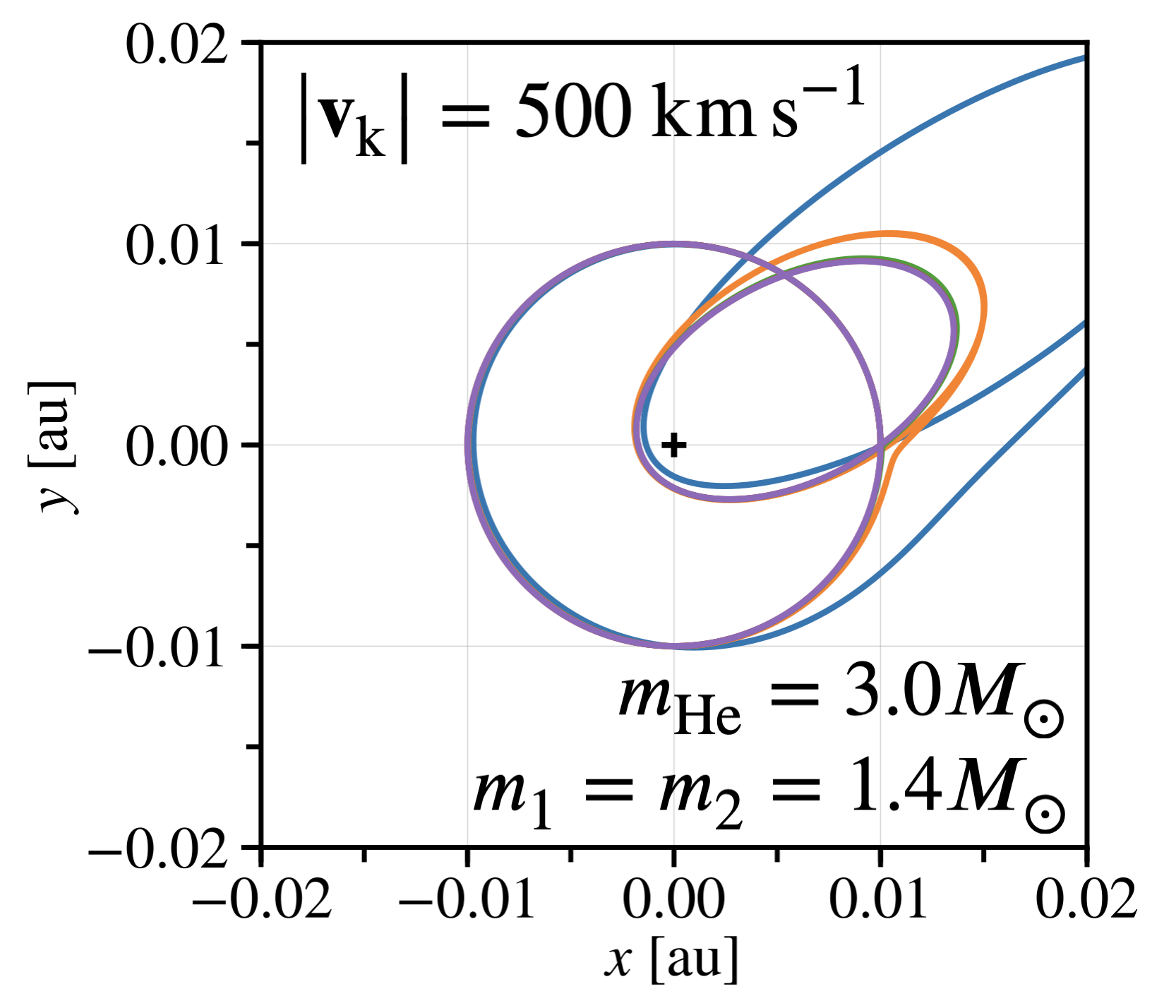
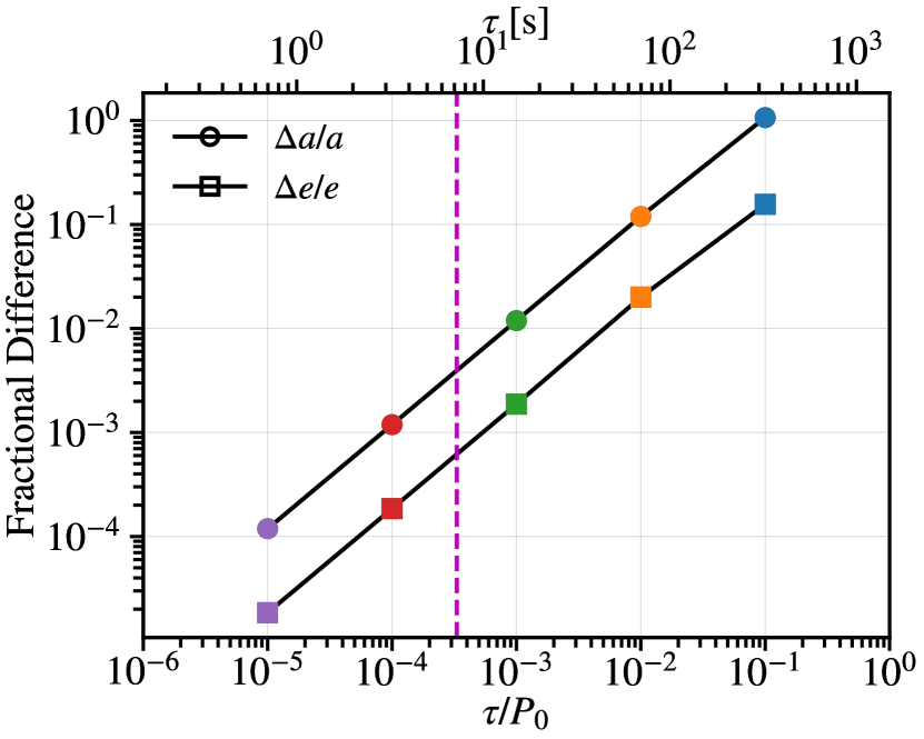
Figure 1: Top panel: orbital trajectories for $\tau/P_{\rm i}=\tau_{\rm m}/P_{\rm i}=\tau_{\rm k}/P_{\rm i}=\left(10^{-5},10^{-4},10^{-3},10^{-2},10^{-1}\right)$. Bottom panel: fractional difference of the predicted semi-major axis $\Delta a/a=|a_{\rm f}-a_{\rm f,EOM}|/a_{\rm f}$ (line with circle markers) and eccentricity $\Delta e/e=|e_{\rm f}-e_{\rm f,EOM}|/e_{\rm f}$ (line with square markers) of the post-SN binary between our model and BPS. The color of each filled circle and filled square corresponds to the color of the orbital trajectory in the top panel. The dashed magenta line is the light-crossing time for the initial circular binary.

The fractional differences of the post-SN semi-major axis and eccentricity between the two models decreases as the timescales decrease, verifying that our model converges to BPS in the limit of instantaneous mass loss and natal kicks.

3.2 GW bursts

The GW signals produced by the SN mass loss and natal kick are bursts: short-duration peaks in the strain. Here, we estimate the GW energy $(E_{\rm GW})$ and the GW angular momentum $(J_{{\rm GW},i})$ radiated during a burst to leading order using

$$E_{\rm GW} \approx\frac{1}{5}\frac{G}{c^{5}}\int_{\Delta t}\dddot{I}_{jk}\dddot{I}_{jk}\ {\rm d}t\ ,$$ (8a)

$$J_{{\rm GW},i} \approx\frac{2}{5}\frac{G}{c^{5}}\int_{\Delta t}\epsilon_{ijk}\ddot{I}_{jm}\dddot{I}_{km}\ {\rm d}t\ ,$$ (8b)

where $\Delta t$ is a chosen time interval centered at the peak of the mass loss and natal kick and $\epsilon_{ijk}$ is the Levi-Civita tensor. We emphasize that this is a leading-order estimate of the GW energy and angular momentum radiated from the SN mass loss and natal kick. Since the kick timescale is much shorter than the mass-loss timescale, we expect that GW emission from the natal kick will be much larger than that from the mass loss.

The observed strain on Earth depends on the orientation of the binary relative to the line of sight. The binary can be randomly oriented with respect to the line of sight, and the kick direction can be randomly oriented with respect to the orbital plane. In the transverse-traceless gauge, the observed strain tensor is

$$h_{jk}^{\rm TT}=\frac{2G}{c^{4}D}\ddot{\cal I}_{jk}^{\rm TT}=\frac{2G}{c^{4}D}\left({\cal P}_{jl}{\cal P}_{km}\ddot{\cal I}_{lm}-\frac{1}{2}{\cal P}_{jk}{\cal P}_{lm}\ddot{\cal I}_{lm}\right)\ ,$$ (9)

where ${\cal I}_{jk}=I_{jk}-\frac{1}{3}\delta_{jk}I_{jk}$ is the reduced quadrupole moment tensor, $D$ is the luminosity distance to the source, and ${\cal P}_{jk}=\delta_{jk}-n_{j}n_{k}$ is the projection tensor from the orbital reference frame to the observer’s frame. We take the unit vector along the line of sight in the observer’s frame to be ${\bf n}=(0,0,1)$. With this line-of-sight orientation, the strain plus and cross polarizations are $h_{+}=h_{xx}=-h_{yy}$ and $h_{\times}=h_{xy}=h_{yx}$, respectively (where $x$ and $y$ here refer to the observer’s frame).

The signal-to-noise ratio (SNR) of the GW burst (prior to modulation by the detector antenna pattern) obeys

$${\rm SNR}=\sqrt{4\int_{-\infty}^{\infty}\frac{|\tilde{h}(f)|^{2}}{{\cal S}(f)}\,{\rm d}f}\ ,$$ (10)

where $f$ is the GW frequency, $\tilde{h}(f)$ is the Fourier-transformed strain and ${\cal S}(f)$ is the detector strain sensitivity. For this work, we ignore Doppler boosting of the observed GW strain and GW frequency due to the motion of the binary relative to the line of sight since the largest natal kick velocities we consider satisfy ${\rm v}_{\rm k}/c\lesssim 1\%$.

A variety of methods have been developed for GW burst detection (e.g., Anderson et al., 2001; Pradier et al., 2001). Here, we are primarily interested in determining the distances at which GW bursts from natal kicks will produce statistically significant excess power in a detector. Often a fiducial SNR threshold of 4.5 for GW burst detectability is used (e.g., Abbott et al., 2016; Macleod et al., 2016), and we adopt this criterion here.

4 Results and Discussion

4.1 Energy and angular momentum in GWs

We first investigate the GW energy and angular momentum distributions for both bound and unbound post-SN binaries, using the mass constraints on GW170817 as a fiducial system. In Table 1, we tabulate the model parameter ranges that we consider. We compute $5{\times}10^{4}$ models for bound binaries and $5{\times}10^{4}$ models for unbound binaries (a total of $10^{5}$ models) with initial parameters sampled from the tabulated distributions.

Parameter	Description	Method
$m_{1}$	Primary NS mass	Uniform $[1.36M_{\odot},1.60M_{\odot}]$
$m_{2}$	Secondary NS mass	Uniform $[1.17M_{\odot},1.36M_{\odot}]$
$m_{\rm He}$	Helium-star mass	Uniform $[2.6M_{\odot},8.0M_{\odot}]$
$a_{\rm i}$	Pre-SN semi-major axis	Log uniform $[0.1R_{\odot},10R_{\odot}]$
${\rm v}_{\rm k}$	SN kick velocity	Uniform $[0.0,2500]\ {\rm km}\,{\rm s}^{-1}$
$\tau_{\rm m}$	Mass-loss timescale	Log uniform $[a_{\rm i}/c,10^{-2}P_{\rm i}]$
$\tau_{\rm k}$	Kick timescale	Log uniform $[0.05,0.5]\ {\rm s}$
$a_{\rm f}$	BPS post-SN semi-major axis	Equation 3a
$e_{\rm f}$	BPS post-SN eccentricity	Equation 3b
$a_{\rm f,EOM}$	EOM post-SN semi-major axis	Equations 5-7
$e_{\rm f,EOM}$	EOM post-SN eccentricity	Equations 5-7

Table 1: Table of model parameters with descriptions and methods with which they are sampled or calculated.

The NS masses are uniformly distributed with $m_{1}\in[1.36M_{\odot},1.60M_{\odot}]$ and $m_{2}\in[1.17M_{\odot},1.36M_{\odot}]$. The mass-loss and kick timescales are sampled log-uniformly in $\left[a_{\rm i}/c,10^{-2}P_{\rm i}\right]$ and $\left[0.05,0.5\right]\,{\rm s}$, respectively. The mass-loss timescale is bounded by the light-crossing time of the binary, and the kick timescales are informed by multi-dimensional core-collapse SN simulations (e.g., Gessner & Janka, 2018). The magnitude of the kick velocities is sampled uniformly in $\left[0,2500\right]\,{\rm km\ s}^{-1}$, with the kick direction sampled isotropically on the unit sphere.

We plot comparisons of GW energy and angular momentum between bound and unbound binaries relative to their initial energy and angular momenta in the top panel of Figure 2.

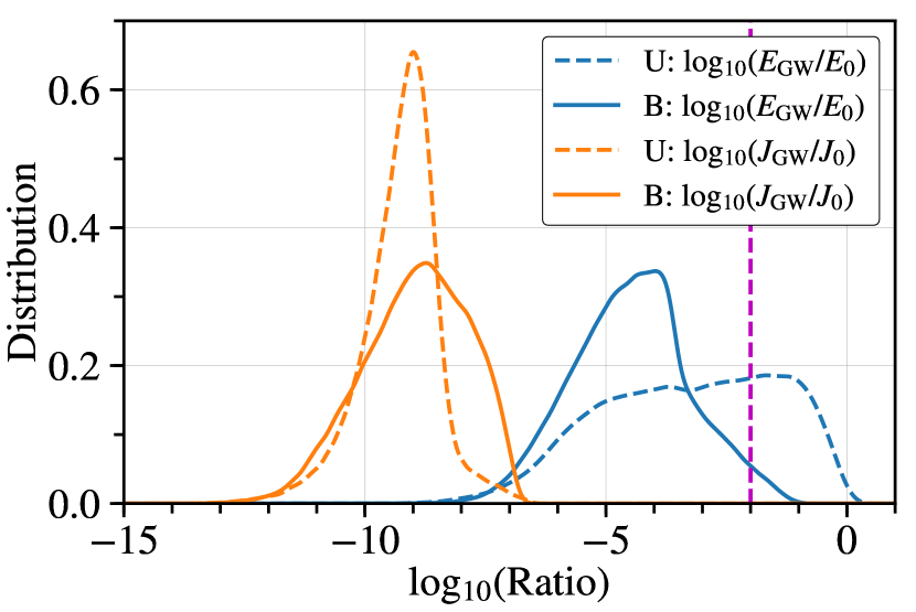
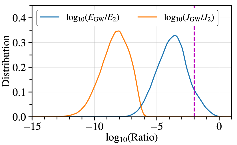
Figure 2: Top panel: distribution of energy and angular momentum radiated in GWs for $5{\times}10^{4}$ bound (B) and $5{\times}10^{4}$ unbound (U) binaries relative to their initial energy and angular momenta. The blue and orange filled lines correspond to the energy and angular-momentum ratios for bound binaries, respectively. The blue and orange dashed lines correspond to the same quantities for unbound binaries. The dashed magenta line corresponds to a value of $1\%$. Bottom panel: distribution of energy and angular momentum radiated in GWs for bound binaries relative to the post-SN binary orbital energy and angular momentum.

The unbound binaries have a larger fraction of GW energy emitted above $1\%$ compared to the bound binaries. This is because larger kick velocities and shorter kick timescales not only are more likely to unbind the binary, they are also more likely to produce larger-amplitude GW bursts. We find that the angular momentum radiated away in GWs is a negligible fraction of the initial binary angular momentum for bound and unbound binaries.

We also plot the the distributions of GW energy and angular momentum relative to those of the post-SN binary. A fraction of bound binaries has an estimated GW energy $\gtrsim 10\%$ of the post-SN binary, so their semi-major axes will be comparably smaller than what BPS would predict, since the latter assumes energy conservation. As for the pre-SN comparison, the angular momentum radiated in GWs is a negligible fraction of the post-SN binary’s angular momentum.

4.2 Detectability

We plot the Fourier-transformed strain for a binary at $D=20\,{\rm Mpc}$ in the top panel of Figure 3 along with the strain sensitivity curves for DECIGO (e.g., Yagi & Seto, 2011) and the Einstein Telescope (e.g., Hild et al., 2011). The Einstein Telescope is designed to be more sensitive to lower frequencies compared to Cosmic Explorer (LIGO-Virgo Collaboration, 2017a).

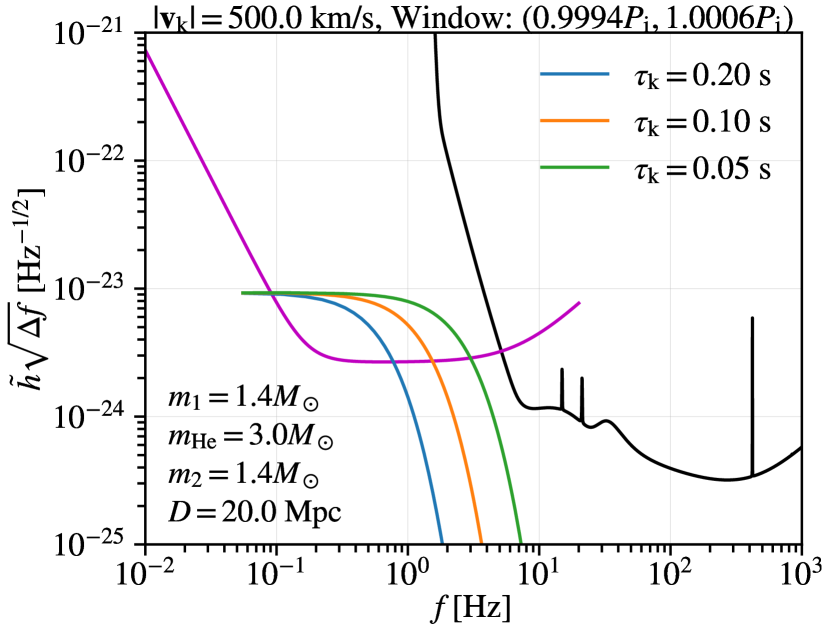
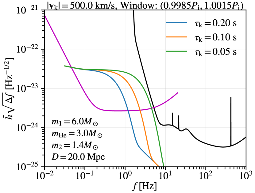
Figure 3: Top panel: Fourier transform of the strain from a kicked binary with $m_{1}=m_{2}=1.4M_{\odot}$, corresponding to a BNS. The blue, orange, and green colors correspond to kick timescales of $\tau_{\rm k}=0.20\,{\rm s}$, $0.10\,{\rm s}$, and $0.05\,{\rm s}$, respectively. The window size for this case is $(0.9994P_{\rm i},1.0006P_{\rm i})$. The magenta and black lines are the sensitivity curves for DECIGO and the Einstein Telescope, respectively. Bottom panel: same as the top panel, but for a binary with $m_{1}=6.0M_{\odot}$, corresponding to a NSBH binary. The window size for this case is $(0.9985P_{\rm i},1.0015P_{\rm i})$.

For shorter natal-kick timescales, the strain spectrum extends to higher GW frequencies, increasing the area between the strain spectrum and the DECIGO sensitivity curve and thus increasing the SNR.

In the bottom panel of Figure 3, we plot Fourier spectra for a NSBH binary with a BH mass of $m_{1}=6.0M_{\odot}$. As expected, natal-kick GW bursts from NSBH binaries will be detectable to larger distances compared to BNSs due to the higher chirp mass. The event rate for NSBH mergers, however, is expected to be lower than that of BNSs (e.g., Mink & Belczynski, 2015; Gupta et al., 2017; Mapelli & Giacobbo, 2018), which implies that the SN event rate for NSBH binaries will also be lower. BBH natal-kick GW bursts would also be detectable to larger distances if BHs receive SN natal kicks with strengths and timescales comparable to NSs.

We now consider how sensitive the SNR of the GW burst is to the initial orientation relative to the line of sight and the kick direction relative to the orbital plane. We sample a total of $10^{6}$ binary configurations, consisting of $10^{3}$ kick directions and for each individual kick direction, $10^{3}$ binary orientations relative to the line of sight. For each configuration, we calculate the SNR of the burst signal (prior to modulation by the detector antenna pattern) at source distances of $D=20\,{\rm Mpc},40\,{\rm Mpc}$, and $80\,{\rm Mpc}$, and plot the corresponding distributions of the SNR in Figure 4.

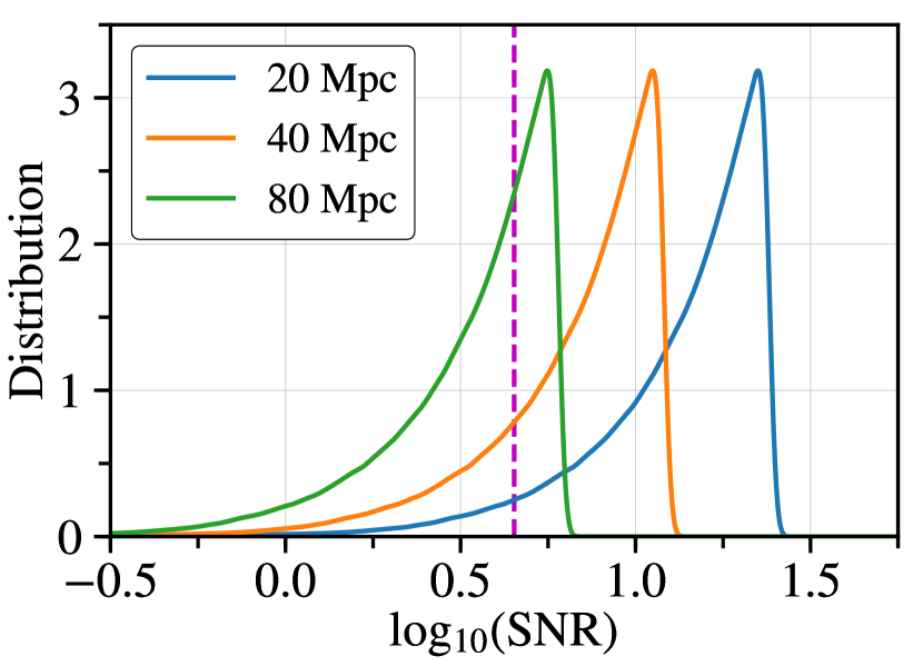
Figure 4: Distributions of the SNR (as calculated via Equation 10) for binary parameters of $m_{1}=m_{2}=1.4M_{\odot}$, $m_{\rm He}=3.0M_{\odot}$, $a_{\rm i}=10^{-2}\ {\rm au}$, $|{\bf v}_{\rm k}|=500\ {\rm km\ s}^{-1}$, and $\tau_{\rm k}=0.1\,{\rm s}$. We sample the kick directions and orbital-plane orientations relative to the line-of-sight isotropically, with $10^{3}$ kick directions and for each kick direction, $10^{3}$ line-of-sight orientations ($10^{6}$ total binary configurations). The blue, orange, and green colors correspond to the SNR being evaluated at sources distances of $D=20\,{\rm Mpc},40\,{\rm Mpc}$, and $80\,{\rm Mpc}$, respectively. The dashed magenta line corresponds to a fiducial SNR threshold of 4.5 for GW burst detectability (e.g., Abbott et al., 2016; Macleod et al., 2016). The SNR distributions are left-skewed with $94\%$, $80\%$, and $37\%$ lying above the SNR threshold for $D=20\,{\rm Mpc},40\,{\rm Mpc}$, and $80\,{\rm Mpc}$, respectively.

The SNR distributions are left-skewed with 94%, 80%, and 37% lying above the fiducial detectability SNR threshold of 4.5 for $D=20\,{\rm Mpc},40\,{\rm Mpc}$, and $80\,{\rm Mpc}$, respectively.

SNe in close binaries can also be followed up with electromagnetic observations, showing promise for multi-messenger science with decihertz GW detectors. Multi-band GW science may also be possible since the core collapse itself will generate GWs at of order hundreds of hertz to kilohertz frequencies. Third-generation ground-based detectors like Einstein Telescope and Cosmic Explorer will be sensitive to GWs from the core collapse out to the Magellanic Clouds (e.g., Roma et al., 2019). We thus expect a helium-star SN explosion with a close NS companion may be a multi-band GW source of interest out to such a distance.

5 Conclusions

SN mass loss and natal kicks are important processes in the formation of compact binaries in isolation. BNSs are expected to primarily form in the field with the immediate progenitor being a helium star/NS system. As the helium star undergoes a SN explosion, the mass loss and natal kick will reorient the binary and may form either a BNS that merges within a Hubble time, a binary that is effectively stalled, or an unbound binary. The SN mass loss and natal kick contribute to the time-varying quadrupole moment of the binary and generate bursts of GWs corresponding to the different timescales of each process.

We have modeled the transition from the pre-SN binary to the post-SN binary by integrating the equation of motion (Equation 5). From our model, we have shown that the SN mass loss and natal kicks that form or unbind BNSs produce GW bursts that may be of interest to next-generation mid-band GW detectors like DECIGO. We find that the energy radiated in the GW burst may be $\gtrsim 10\%$ of the post-SN orbital energy, while the angular momentum radiated away in GWs is negligible, i.e., $\lesssim 10^{-3}\%$. It may thus be important to include GW backreaction on the post-SN binary in BPS codes and to determine how this addition affects the expected populations of low-mass X-ray binaries, Galactic binary pulsars, and the merging compact binaries that LIGO detects.

For future work, we will investigate natal kicks in the isolated-binary channel for BBHs and extend the analysis we present here to a more self-consistent post-Newtonian model for the equation of motion. We will also investigate how important the 3D hydrodynamical effects may be during the pre-SN to post-SN binary transition as the ejecta leave the binary.

References

- Abbott et al. (2016) Abbott B. P., et al., 2016, Living Rev. Relativ., 19
- Anderson et al. (2001) Anderson W. G., Brady P. R., Creighton J. D. E., Flanagan É. É., 2001, PRD, 63, 042003
- Andresen et al. (2017) Andresen H., Müller B., Müller E., Janka H.-T., 2017, MNRAS, 468, 2032
- Andresen et al. (2019) Andresen H., Müller E., Janka H.-T., Summa A., Gill K., Zanolin M., 2019, MNRAS, 486, 2238
- Andrews & Mandel (2019) Andrews J. J., Mandel I., 2019, ApJL, 880, L8
- Andrews & Zezas (2019) Andrews J. J., Zezas A., 2019, MNRAS, 486, 3213
- Andrews et al. (2015) Andrews J. J., Farr W. M., Kalogera V., Willems B., 2015, ApJ, 801, 32
- Atri et al. (2019) Atri P., et al., 2019, arXiv:1908.07199 [astro-ph]
- Barrett et al. (2018) Barrett J. W., Gaebel S. M., Neijssel C. J., Vigna-Gómez A., Stevenson S., Berry C. P. L., Farr W. M., Mandel I., 2018, MNRAS, 477, 4685
- Belczyński & Bulik (1999) Belczyński K., Bulik T., 1999, A&A, 346, 91
- Beniamini et al. (2016) Beniamini P., Hotokezaka K., Piran T., 2016, ApJL, 829, L13
- Brandt & Podsiadlowski (1995) Brandt N., Podsiadlowski P., 1995, MNRAS, 274, 461
- Bray & Eldridge (2016) Bray J. C., Eldridge J. J., 2016, MNRAS, 461, 3747
- Bray & Eldridge (2018) Bray J. C., Eldridge J. J., 2018, MNRAS, 480, 5657
- Burrows & Hayes (1996) Burrows A., Hayes J., 1996, PRL, 76, 352
- Colpi & Wasserman (2002) Colpi M., Wasserman I., 2002, ApJ, 581, 1271
- Coulter et al. (2017) Coulter D. A., et al., 2017, Science, 358, 1556
- De et al. (2018) De K., et al., 2018, Science, 362, 201
- Dewi et al. (2002) Dewi J. D. M., Pols O. R., Savonije G. J., van den Heuvel E. P. J., 2002, MNRAS, 331, 1027
- Dominik et al. (2012) Dominik M., Belczynski K., Fryer C., Holz D. E., Berti E., Bulik T., Mandel I., O’Shaughnessy R., 2012, ApJ, 759, 52
- Fragos et al. (2013) Fragos T., et al., 2013, ApJ, 764, 41
- Fragos et al. (2019) Fragos T., Andrews J. J., Ramirez-Ruiz E., Meynet G., Kalogera V., Taam R. E., Zezas A., 2019, arXiv:1907.12573 [astro-ph]
- Fryer & Kalogera (1997) Fryer C., Kalogera V., 1997, ApJ, 489, 244
- Fryer & Kusenko (2006) Fryer C. L., Kusenko A., 2006, ApJS, 163, 335
- Fryer & New (2003) Fryer C. L., New K. C. B., 2003, Liv. Rev. Relativ., 6, 2
- Fryer et al. (2004) Fryer C. L., Holz D. E., Hughes S. A., 2004, ApJ, 609, 288
- Fryxell & Arnett (1981) Fryxell B. A., Arnett W. D., 1981, ApJ, 243, 994
- Gessner & Janka (2018) Gessner A., Janka H.-T., 2018, ApJ, 865, 61
- Giacobbo & Mapelli (2018) Giacobbo N., Mapelli M., 2018, MNRAS, 480, 2011
- Gossan et al. (2016) Gossan S., Sutton P., Stuver A., Zanolin M., Gill K., Ott C., 2016, PRD, 93, 042002
- Gupta et al. (2017) Gupta A., Arun K. G., Sathyaprakash B. S., 2017, ApJL, 849, L14
- Hallinan et al. (2017) Hallinan G., et al., 2017, Science, 358, 1579
- Hild et al. (2011) Hild S., et al., 2011, CQG, 28, 094013
- Hills (1983) Hills J. G., 1983, ApJ, 267, 322
- Hobbs et al. (2005) Hobbs G., Lorimer D. R., Lyne A. G., Kramer M., 2005, MNRAS, 360, 974
- Holgado & Ricker (2019) Holgado A. M., Ricker P. M., 2019, ApJ, 882, 39
- Holgado et al. (2018) Holgado A. M., Ricker P. M., Huerta E. A., 2018, ApJ, 857, 38
- Holland-Ashford et al. (2017) Holland-Ashford T., Lopez L. A., Auchettl K., Temim T., Ramirez-Ruiz E., 2017, ApJ, 844, 84
- Hurley et al. (2002) Hurley J. R., Tout C. A., Pols O. R., 2002, MNRAS, 329, 897
- Iben & Tutukov (1996) Iben I., Tutukov A. V., 1996, ApJ, 456, 738
- Ivanova et al. (2003) Ivanova N., Belczynski K., Kalogera V., Rasio F. A., Taam R. E., 2003, ApJ, 592, 475
- Janka (2013) Janka H.-T., 2013, MNRAS, 434, 1355
- Janka (2017) Janka H.-T., 2017, ApJ, 837, 84
- Janka & Müller (1994) Janka H.-T., Müller E., 1994, A&A, 290, 496
- Kalogera (1996) Kalogera V., 1996, ApJ, 471, 352
- Kasliwal et al. (2017) Kasliwal M. M., et al., 2017, Science, 358, 1559
- Katsuda et al. (2018) Katsuda S., et al., 2018, ApJ, 856, 18
- Kochanek et al. (2019) Kochanek C. S., Auchettl K., Belczynski K., 2019, MNRAS, 485, 5394
- Kruckow et al. (2018) Kruckow M. U., Tauris T. M., Langer N., Kramer M., Izzard R. G., 2018, MNRAS, 481, 1908
- Kusenko (2004) Kusenko A., 2004, IJMPD, 13, 2065
- Kusenko & Segrè (1996) Kusenko A., Segrè G., 1996, PRL, 77, 4872
- LIGO-Virgo Collaboration (2016a) LIGO-Virgo Collaboration 2016a, PRL, 116, 061102
- LIGO-Virgo Collaboration (2016b) LIGO-Virgo Collaboration 2016b, PRL, 116, 241103
- LIGO-Virgo Collaboration (2017a) LIGO-Virgo Collaboration 2017a, CQG, 34, 044001
- LIGO-Virgo Collaboration (2017b) LIGO-Virgo Collaboration 2017b, PRL, 119, 161101
- LIGO-Virgo Collaboration (2017c) LIGO-Virgo Collaboration 2017c, ApJL, 850, L40
- MacLeod & Ramirez-Ruiz (2014) MacLeod M., Ramirez-Ruiz E., 2014, ApJL, 798, L19
- Macleod et al. (2016) Macleod D., Harry I., Fairhurst S., 2016, PRD, 93, 064004
- Mandel (2016) Mandel I., 2016, MNRAS, 456, 578
- Mapelli & Giacobbo (2018) Mapelli M., Giacobbo N., 2018, MNRAS, 479, 4391
- Martin et al. (2009) Martin R. G., Tout C. A., Pringle J. E., 2009, MNRAS, 397, 1563
- Michaely & Perets (2018) Michaely E., Perets H. B., 2018, ApJL, 855, L12
- Mink & Belczynski (2015) Mink S. E. d., Belczynski K., 2015, ApJ, 814, 58
- Morozova et al. (2018) Morozova V., Radice D., Burrows A., Vartanyan D., 2018, ApJ, 861, 10
- Müller et al. (2018) Müller B., Gay D. W., Heger A., Tauris T. M., Sim S. A., 2018, MNRAS, 479, 3675
- Müller et al. (2019) Müller B., et al., 2019, MNRAS, 484, 3307
- Nakamura et al. (2019) Nakamura K., Takiwaki T., Kotake K., 2019, PASJ, submitted (arXiv:1904.08088)
- Nordhaus et al. (2010) Nordhaus J., Brandt T. D., Burrows A., Livne E., Ott C. D., 2010, PRD, 82, 103016
- Nordhaus et al. (2012) Nordhaus J., Brandt T. D., Burrows A., Almgren A., 2012, MNRAS, 423, 1805
- O’Shaughnessy et al. (2005) O’Shaughnessy R., Kim C., Fragos T., Kalogera V., Belczyński K., 2005, ApJ, 633, 1076
- O’Shaughnessy et al. (2017) O’Shaughnessy R., Gerosa D., Wysocki D., 2017, PRL, 119
- Osłowski et al. (2011) Osłowski S., Bulik T., Gondek-Rosińska D., Belczyński K., 2011, MNRAS, 413, 461
- Pajkos et al. (2019) Pajkos M. A., Couch S. M., Pan K.-C., O’Connor E. P., 2019, ApJ, 878, 13
- Postnov & Yungelson (2006) Postnov K. A., Yungelson L. R., 2006, Living Rev. Relativ., 9, 6
- Powell & Müller (2019) Powell J., Müller B., 2019, MNRAS, 487, 1178
- Powell et al. (2016) Powell J., Gossan S. E., Logue J., Heng I. S., 2016, PRD, 94, 123012
- Pradier et al. (2001) Pradier T., Arnaud N., Bizouard M.-A., Cavalier F., Davier M., Hello P., 2001, PRD, 63, 042002
- Radice et al. (2019) Radice D., Morozova V., Burrows A., Vartanyan D., Nagakura H., 2019, ApJL, 876, L9
- Repetto et al. (2012) Repetto S., Davies M. B., Sigurdsson S., 2012, MNRAS, 425, 2799
- Roma et al. (2019) Roma V., Powell J., Heng I. S., Frey R., 2019, PRD, 99, 063018
- Sagert & Schaffner-Bielich (2008) Sagert I., Schaffner-Bielich J., 2008, A&A, 489, 281
- Sato et al. (2009) Sato S., et al., 2009, J. Phys.: Conf. Ser., 154, 012040
- Sato et al. (2017) Sato S., et al., 2017, J. Phys.: Conf. Ser., 840, 012010
- Scheck et al. (2004) Scheck L., Plewa T., Janka H.-T., Kifonidis K., Müller E., 2004, PRL, 92, 011103
- Scheck et al. (2006) Scheck L., Kifonidis K., Janka H.-T., Müller E., 2006, A&A, 457, 963
- Schinzel et al. (2019) Schinzel F. K., Kerr M., Rau U., Bhatnagar S., Frail D. A., 2019, ApJL, 876, L17
- Socrates et al. (2005) Socrates A., Blaes O., Hungerford A., Fryer C. L., 2005, ApJ, 632, 531
- Tauris et al. (2013) Tauris T. M., Langer N., Moriya T. J., Podsiadlowski P., Yoon S.-C., Blinnikov S. I., 2013, ApJL, 778, L23
- Tauris et al. (2015) Tauris T. M., Langer N., Podsiadlowski P., 2015, MNRAS, 451, 2123
- Tauris et al. (2017) Tauris T. M., et al., 2017, ApJ, 846, 170
- Taylor & Gerosa (2018) Taylor S. R., Gerosa D., 2018, PRD, 98, 083017
- Tzanavaris et al. (2013) Tzanavaris P., et al., 2013, ApJ, 774, 136
- Vigna-Gómez et al. (2018) Vigna-Gómez A., et al., 2018, MNRAS, 481, 4009
- Wang et al. (2006) Wang C., Lai D., Han J. L., 2006, ApJ, 639, 1007
- Wheeler et al. (1975) Wheeler J. C., Lecar M., McKee C. F., 1975, ApJ, 200, 145
- Willems et al. (2004) Willems B., Kalogera V., Henninger M., 2004, ApJ, 616, 414
- Wong et al. (2010) Wong T.-W., Willems B., Kalogera V., 2010, ApJ, 721, 1689
- Wongwathanarat et al. (2010) Wongwathanarat A., Janka H.-T., Müller E., 2010, ApJL, 725, L106
- Wongwathanarat et al. (2013) Wongwathanarat A., Janka H.-T., Müller E., 2013, A&A, 552, A126
- Wysocki et al. (2018) Wysocki D., Gerosa D., O’Shaughnessy R., Belczynski K., Gladysz W., Berti E., Kesden M., Holz D. E., 2018, PRD, 97, 043014
- Yagi & Seto (2011) Yagi K., Seto N., 2011, PRD, 83, 044011