Operator content of entanglement spectra after global quenches in the transverse field Ising chain

Abstract

We consider the time evolution of the gaps of the entanglement spectrum for a block of consecutive sites in finite transverse field Ising chains after sudden quenches of the magnetic field. We provide numerical evidence that, whenever we quench at or across the quantum critical point, the time evolution of the ratios of these gaps allows to obtain universal information. They encode the low-lying gaps of the conformal spectrum of the Ising boundary conformal field theory describing the spatial bipartition within the imaginary time path integral approach to global quenches at the quantum critical point.

Quantum many-body systems described by local Hamiltonians are difficult to solve because the dimensionality of their Hilbert space increases exponentially with the number of their constituents. At equilibrium however the wave-functions of quantum many-body systems described by gapped Hamiltonians contain a limited amount of entanglement with a well defined structure that can be used to perform numerical simulations with tensor networks Hastings (2007); Masanes (2009); Amico et al. (2008); Bridgeman and Chubb (2017); Orús (2014); Ran et al. (2017). At quantum critical points (QCP), where the Hamiltonians become gapless, the entanglement grows following universal laws Pelissetto and Vicari (2002) that in the specific case of conformal invariant QCP allow to unveil the data of the underlying conformal field theory (CFT) Belavin et al. (1984); Henkel (1999). In two spacetime dimensions, these data include the central charge $c$, the exponents dictating the decay of correlation functions that constitute the conformal spectrum and the coefficients of the operator product expansion. The central charge $c$ can be read from the scaling of the entanglement entropy (EE) of an interval with respect to its size Holzhey et al. (1994); Calabrese and Cardy (2004); Vidal et al. (2003); Callan and Wilczek (1994). The remaining CFT data are encoded e.g. in the EE when $A$ is made by disjoint intervals Calabrese et al. (2009, 2011); Alba et al. (2011); Coser et al. (2014a); De Nobili et al. (2015), in a complicated way. The entanglement spectrum (ES) Li and Haldane (2008); Peschel and Truong (1987); Calabrese and Lefevre (2008); Poilblanc (2010); Cirac et al. (2011); Dubail et al. (2012); Läuchli (2013), i.e. the spectrum of the reduced density matrix, can be related to the conformal spectrum of a conformal field theory with boundaries (BCFT) defined by proper conformal boundary conditions (CBC) Cardy and Tonni (2016), as also observed by Läuchli in numerical studies Läuchli (2013).

Entanglement plays a central role in our understanding of large many-body quantum systems, as witnessed by the numerous proposals on how to measure entanglement in experiments which have led to the first experimental measures in the context of cold atoms and trapped ions both at and out of equilibrium Cardy (2011); Abanin and Demler (2012); Daley et al. (2012); Islam et al. (2015); Hauke et al. (2016); Pichler et al. (2016); Kaufman et al. (2016); Brydges et al. (2019); Lukin et al. (2019). Such experiments are expected to play an increasingly important role out of equilibrium, where the amount of entanglement increases to its maximum value very fast with time Calabrese and Cardy (2005); De Chiara et al. (2006); Nahum et al. (2017). This creates an entanglement barrier that prevents to extract reliable predictions at long time even when using our best classical-simulation techniques Vidal (2004); White and Feiguin (2004); Daley et al. (2004); Paeckel et al. (2019) (see Leviatan et al. (2017); White et al. (2017); Surace et al. (2019); Rams and Zwolak (2019); Krumnow et al. (2019) for recent proposals to overcome this barrier).

As a result, important questions about strongly correlated quantum many-body quantum systems out of equilibrium are only partially understood and currently can only be settled experimentally. Examples of open questions include the existence of new phases of matter out of equilibrium Fausti et al. (2011); Abanin and Papić (2017); Alet and Laflorencie (2018), the presence/absence of equilibration, the phenomenon of thermalization or generalized thermalisation that should reconcile the reversibility of quantum mechanics with the irreversibility of the macroscopic world Rigol et al. (2008); Polkovnikov et al. (2011); Eisert et al. (2015); D’Alessio et al. (2016). A possible hope is that also out of equilibrium a form of universality exists. This would allow for example to obtain at least quantitative information even with approximate algorithms.

Out of equilibrium universality has been observed only in some specific scenarios where the scaling of the spatio-temporal evolution of the system can be described by universal exponents and functions (see the recent experiment Prüfer et al. (2018) and the references therein). Dynamical quantum phase transitions, appearing as singularities in the return probabilities to the initial state quenched across a quantum critical point, could also provide a scaling region that could be explained through out-of-equilibrium universality Heyl et al. (2013); Žunkovič et al. (2018); Heyl (2019).

In this Letter we consider the spin-$\tfrac{1}{2}$ transverse field Ising chain (TFIC), a paradigmatic model for one-dimensional quantum critical behaviour and quantum phase transitions. We study the time evolutions of the ES after a global quench given by a sudden change of the magnetic field, when the subsystem $A$ is an interval in a finite system. We provide numerical evidence that, for quenches to or across the QCP, the gaps of the ES carry information about the conformal spectrum of the Ising BCFT describing the QCP. These results are quite robust under changes of the quench protocol thus providing a new example of universality out of equilibrium.

Setup.

The Hamiltonian of the TFIC is

$$H(\theta)=-\,\frac{1}{2}\left(\,\sum_{i=1}^{L-1}\sigma_{i}^{x}\sigma_{i+1}^{x}+\cot\theta\sum_{i=1}^{L}\sigma_{i}^{z}+\eta\,\sigma^{x}_{L}\sigma^{x}_{1}\right)$$ (1)

where $\sigma_{i}^{\alpha}$ are the Pauli matrices at the $i$-th site and $\cot\theta$ is the magnetic field, with $0<\theta<\tfrac{\pi}{2}$. At zero temperature and in the thermodynamic limit, this model exhibits a ferromagnetic (ordered) phase for $\tfrac{\pi}{4}<\theta<\tfrac{\pi}{2}$ and a paramagnetic (disordered) phase for $0<\theta<\tfrac{\pi}{4}$, separated by a QCP at $\theta=\tfrac{\pi}{4}$. We consider finite systems made by $L$ sites where either periodic boundary conditions (PBC) or free open boundary conditions (OBC) are imposed, which correspond respectively to $\eta=1$ and $\eta=0$ in (1).

Entanglement can be studied by partitioning the system into an interval $A$ made by $\ell<L/2$ consecutive sites and its complement $B$ (in the case of OBC, $d$ denotes the number of sites on the left of $A$). Assuming that the Hilbert space can accordingly be written as $\mathcal{H}=\mathcal{H}_{A}\otimes\mathcal{H}_{B}$, we are interested in the ES, i.e. in the eigenvalues $\lambda_{i}\equiv e^{-\xi_{i}}$ (where $\xi_{i}\geqslant 0$) of the reduced density matrix $\rho_{A}=\textrm{Tr}_{\mathcal{H}_{B}}\rho$ (normalised by $\textrm{Tr}_{\mathcal{H}_{A}}\rho_{A}=1$) of $A$. In order to get rid of arbitrary entanglement energy shifts we consider the gaps $g_{r}\equiv\log\lambda_{\textrm{\tiny max}}-\log\lambda_{r}=\xi_{r}-\xi_{\textrm{\tiny min}}\geqslant 0$ with $r\geqslant 1$. The EE of $A$ is $S_{A}=-\textrm{Tr}_{\mathcal{H}_{A}}(\rho_{A}\log\rho_{A})$. Given the system in the ground state $|\psi_{0}\rangle$ of (1) for $\theta=\theta_{0}$, at $t=0$ the magnetic field is changed abruptly $\theta_{0}\to\theta$, hence the time evolved state is $|\psi(t)\rangle=e^{-\textrm{i}\,H(\theta)\,t}|\psi_{0}\rangle$.

In spectroscopy the ratios $g_{r}/g_{s}$ are usually studied in order to get rid of a shift and a rescaling of the entire spectrum. These quantities are suggested also by the analytic expressions for the time evolution of the ES of half of an infinite line obtained through CFT methods when the post-quench Hamiltonian is critical Cardy and Tonni (2016), which tell us that $(\ell g_{r})^{-1}$ and $g_{r}S_{A}$ depend on critical exponents. We study the time evolutions of $g_{r}/g_{1}$, of $(\ell g_{r})^{-1}$ and of $g_{r}S_{A}$ after global quenches of the magnetic field in the TFIC for various $\theta_{0}$ and $\theta$, showing the numerical results for the first $16$ eigenvalues (hence $r=1,2,\dots,15$). The numerical analysis is performed by using the standard mapping of the TFIC to a chain of free fermions Jordan and Wigner (1928); Lieb et al. (1961); Barouch et al. (1970); Barouch and McCoy (1971a, b) (see also Surace et al. (2019) and references therein). The time evolutions of these quantities after some global quenches have been recently studied in an infinite harmonic chain or in an infinite chain of free fermions at half filling Di Giulio et al. (2019).

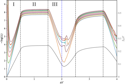
Figure 1: (color online). Time evolutions of the first 16 eigenvalues $\lambda_{\textrm{\tiny max}}\geqslant\lambda_{1}\geqslant\lambda_{2}\geqslant\dots\geqslant\lambda_{15}$ of the ES and of the EE (grey line) for an interval with $\ell=64$ sites in the chain with $L=256$ sites and PBC after the quench $\theta=\pi/8\to\theta=\pi/4$ to the QCP. Different degeneracies are observed in the regimes I, II and III within the period.

Quenches at the QCP.

We report numerical results for the quench $\theta_{0}=\pi/8\to\theta=\pi/4$, from the ferromagnetic phase to the quantum critical point, since they are paradigmatic for generic quenches to the critical point obtained for different choices of $\theta_{0}$. The interval $A$ is either in the chain with PBC (Fig. 1 and Fig. 2) or in the chain with OBC and $d=0$ (Fig. 3) or $d=\tfrac{3}{2}\ell$ (Fig. 4). In the time evolutions of the ES and of the EE in Fig. 1, we see several time regimes (separated by black dashed-dotted vertical lines), that can be identified by employing the quasi-particle picture Calabrese and Cardy (2005, 2006, 2007). It assumes that each spatial point emits a pair of oppositely moving and initially entangled quasi-particles that propagate semiclassically with velocity $v_{\textrm{\tiny q}}=\textrm{min}(1,\cot\theta)$ after the quench Robinson (1976); Bratteli and Robinson (1981). In finite systems this implies quantum recurrences: the quasi-particles emitted at the same point meet periodically at times that are multiple integers of $\tfrac{L/2}{v_{\textrm{\tiny q}}}$ for PBC and of $\tfrac{L}{v_{\textrm{\tiny q}}}$ for OBC (in the figures the end of a period corresponds to the blue dashed-dotted vertical line) Cardy (2014, 2016); Takayanagi and Ugajin (2010); da Silva et al. (2015). When $A$ is an interval in the chain with PBC (Fig. 1, Fig. 2, Fig. 5 and Fig. 6), we can identify three regimes I, II, III ending respectively at $t_{1}=\tfrac{\ell/2}{v_{\textrm{q}}}$ (equilibration time), $t_{2}=\tfrac{(L-\ell)/2}{v_{\textrm{q}}}$ and $t_{3}=\tfrac{L/2}{v_{\textrm{q}}}$. When $A$ is in the chain with OBC and $d=0$ (Fig. 3) these values must be just multiplied by a factor of $2$, while for $d\neq 0$ with $d+\ell<L/2$ (Fig. 4) the bounces of the quasi-particles at the boundaries provide nine regimes I, II, …, IX within a period.

The time evolutions in Fig. 2, Fig. 3 and Fig. 4 display some interesting common features. For $(\ell g_{r})^{-1}$ (top panels) we observe either linear growths or plateaux or linear decreases in the different regimes, in correspondence of the same behaviour in the EE, with the crucial difference that $(\ell g_{r})^{-1}$ display a higher degree of flatness than EE in regime II, up to oscillations. Understanding the origin of this difference in terms of a Generalised Gibbs Ensemble Rigol et al. (2006, 2007) (see Vidmar and Rigol (2016) for a recent review) could be very insightful.

As for the products $g_{r}S_{A}$ (bottom panels), their time evolutions in regimes I and II approximatively take constant values while they become very complicated in the regimes different from I whenever $(\ell g_{r})^{-1}$ either increase or decrease linearly.

The most interesting behaviour is displayed by the ratios $g_{r}/g_{1}$: up to oscillations, they take approximatively constant values in the different time regimes and the same constant values are observed also in the corresponding regimes of the second period. It is crucial to remark that these constant values are positive integers. Focussing on the regimes I and II, we stress that the integer $1$ is observed only in the regime I in the case of PBC. Furthermore, we find it worth observing the changes of degeneracies in passing from a regime to the subsequent one for PBC in Fig. 2 and for OBC in Fig. 4 (from I to II and from VIII to IX). In particular, for PBC, the higher degeneracy in regime III leads to observe that this regime looks like the time reversal of regime I of the second period. Similarly, the degeneracies seem to tell that the regime I in the first period could be related to the regime III in the second period, maybe because for PBC the quasi-particles come back to their emission point at the end of the second period. Comparing the regimes II in Fig. 2 and Fig. 3, we observe that the plateaux for $(\ell g_{r})^{-1}$ have the same heights. In Fig. 4, where OBC are imposed and $d>\tfrac{\ell}{2}$, the ratios $g_{r}/g_{1}$ take almost constant integer values and the regimes I and II are like in Fig. 2, where PBC are imposed.

A remarkable feature of the time evolutions of $g_{r}/g_{1}$ in Fig. 2 and Fig. 3 is their very mild dependence on the initial state within the paramagnetic phase: changing $0<\theta_{0}<\pi/2$ (we have considered $\theta_{0}=\pi/13$ and $\theta_{0}=\pi/10$ J. Surace et al. ) the same integer constant values with the same degeneracies occur. For PBC the same observation can be made taking initial states within the ferromagnetic phase (we have considered $\theta_{0}=\pi/2-\pi/13$ and $\theta_{0}=\pi/2-\pi/10$): only the degeneracies change with respect to the cases with $0<\theta_{0}<\pi/2$. Instead, for OBC when $d=0$, taking different $\pi/4<\theta_{0}<\pi/2$ we find that the regime II is the same, while in the regime I all the integer values (including $1$) are taken by $g_{r}/g_{1}$, and that the degeneracies change passing from regime I to regime II. Thus, regime II in the time evolutions of the ratios $g_{r}/g_{1}$ in Fig. 2 and Fig. 3 is independent of the initial state. A mild dependence on the initial state occurs in the peak that $g_{r}/g_{1}$ display at the beginning of regime 1. Furthermore, $g_{r}S_{A}$ take different approximatively constant values for different initial states, as observed also in harmonic chains Di Giulio et al. (2019).

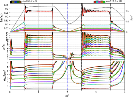
Figure 2: (color online). Time evolution of $(\ell g_{r})^{-1}$ (top), $g_{r}/g_{1}$ (middle) and $g_{r}S_{A}$ (bottom) after the quench $\theta_{0}=\pi/8\to\theta=\pi/4$ for an interval in the chain with PBC.

Insights from BCFT.

Analytic CFT expressions for the time evolutions of the ES in Fig. 2, Fig. 3 and Fig. 4 are not available in the literature. Nonetheless, some of their characteristic features can be justified through the CFT analysis performed in Cardy and Tonni (2016) for the ES of half of the infinite line, based on BCFT Cardy (1986, 1989). The continuum limit of the TFIC at the QCP is described by the Ising CFT, whose central charge is $c=\tfrac{1}{2}$. In the presence of boundaries, the conformal symmetry of the Ising BCFT allows only three CBC.

In the BCFT approach to global quantum quenches with critical evolution Hamiltonians Calabrese and Cardy (2005, 2006, 2007); Cardy (2014, 2016) (see Calabrese and Cardy (2016) for a recent review), the spacetime to consider in the imaginary time path integral is a strip whose width is given by $\tau_{0}$ along the imaginary time direction and by the size of the system along the spatial direction. On both the lines delimiting the strip in the imaginary time direction, the state $|\psi_{0}\rangle$ is approximated by the conformal boundary state $|\tilde{\psi}_{0}\rangle$ corresponding to some CBC $b_{0}$, while the CBC $b_{1}$ and $b_{2}$ are imposed along the parallel segments corresponding to the physical boundaries (for the OBC that we consider $b_{1}=b_{2}\equiv b$, given by free boundary conditions).

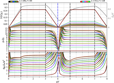
Figure 3: (color online). Time evolution of $(\ell g_{r})^{-1}$ (top), $g_{r}/g_{1}$ (middle) and $g_{r}S_{A}$ (bottom) after the quench $\theta_{0}=\pi/8\to\theta=\pi/4$ for an interval in the chain with OBC, for $d=0$.

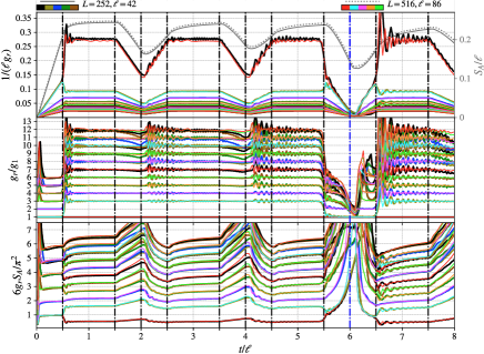
Figure 4: (color online). Time evolution of $(\ell g_{r})^{-1}$ (top), $g_{r}/g_{1}$ (middle) and $g_{r}S_{A}$ (bottom) after the quench $\theta_{0}=\pi/8\to\theta=\pi/4$ for an interval made by $\ell$ sites in the chain with OBC, for $d=\tfrac{3}{2}\ell$.

Following Cardy and Tonni (2016) (see also Holzhey et al. (1994); Peschel (2004a); Ohmori and Tachikawa (2015); Alba et al. (2017); Tonni et al. (2018); Wen et al. (2018)), it is convenient to regularise the ultraviolet (UV) divergencies by removing small disks centered at the entangling points whose radius is the infinitesimal UV cutoff $\epsilon$. This introduces a boundary around each entangling point, where the CBC $a$ is imposed.

When the subsystem $A$ is half of the infinite line, the spacetime can be conformally mapped into an annulus whose CBC are $a$ and $b_{0}$. After a crucial analytic continuation to real time, in this case one finds $1/g_{r}=(2\pi\tau_{0}\,\Delta_{r})^{-1}t$ grow linearly in time and $g_{r}/g_{1}=\Delta_{r}/\Delta_{1}$ are independent of time, where $r\geqslant 1$ and $\Delta_{r}\in\mathcal{S}(a,b_{0})\setminus\{0\}$, being $\mathcal{S}(a,b_{0})$ the conformal spectrum (made by the conformal dimensions of the primary fields and of their descendants) of the BCFT on the annulus with CBC given by $a$ and $b_{0}$ Cardy and Tonni (2016). The parameter $\tau_{0}$ encodes information about the initial state. Furthermore, the linear growth of the EE for this bipartition Calabrese and Cardy (2005, 2006, 2007) leads to $g_{r}\,S_{A}=\tfrac{\pi^{2}c}{3}\,\Delta_{r}$, which is independent of time. We remark that $g_{r}/g_{1}$ and $g_{r}\,S_{A}$ are independent of $\tau_{0}$.

When the system is finite and the subsystem $A$ has $N$ entangling points ($N$ must be even for PBC), the spacetime has the topology of a sphere with $N+2$ boundaries for PBC and with $N+1$ boundaries for OBC. We expect that, at the beginning (regime I), the time evolution of the ES is determined only by the spacetime around the entangling points. This assumption leads to consider $N$ independent copies of the spacetime corresponding to the time evolution of half of the infinite line; hence to employ the conformal spectrum $\mathcal{S}_{N}(a,b_{0})$ of $N$ independent copies of the same BCFT on the annulus with CBC given by $a$ and $b_{0}$. Combining this assumption with the results of Cardy (1989) and assigning free boundary conditions to both $a$ and $b_{0}$, we can explain the data observed in the regimes I of Fig. 2, Fig. 3 and Fig. 4, where $N=2$, $N=1$ and $N=2$ respectively. This assignment for $a$ has been found also through the numerical analysis of the ES for some bipartitions at equilibrium Läuchli (2013). We remark that also $b$ corresponds to free boundary conditions in our numerical analysis. These assignments lead to $\mathcal{S}(a,b_{0})=\mathcal{S}(a,a)=\mathcal{S}(a,b)=\{0,\tfrac{1}{2},\tfrac{3}{2},2,\tfrac{5}{2},3,\tfrac{7}{2},4,\tfrac{9}{2},5,\dots\}$ (for recent numerical results see Evenbly et al. (2010); Evenbly and Vidal (2014)), which implies that $\mathcal{S}_{N}(a,b_{0})=\{0,\tfrac{1}{2},1,\tfrac{3}{2},2,\tfrac{5}{2},3,\tfrac{7}{2},4,\tfrac{9}{2},5,\dots\}$ for any $N$. For the regime I, this naive BCFT analysis leads to $g_{r}\,S_{A}=\tfrac{\pi^{2}c_{\textrm{\tiny tot}}}{3}\,\Delta_{r}$ where $c_{\textrm{\tiny tot}}=Nc$ and $\Delta_{r}\in\mathcal{S}_{N}(a,b_{0})\setminus\{0\}$. The independence of time is observed from the data, but the numerical values of the constants depend on the initial state, as remarked above. This dependence on the initial state could be justified by arguing that $S_{A}$ and the gaps $g_{r}$ lead to different numerical values for $\tau_{0}$, as already noticed for the linear growths of the Rényi entropies with different values of the Rényi index Coser et al. (2014b).

The quasi-particle picture allows to argue that the regimes II are not influenced by the finite size of the system for the chosen bipartitions, where $\ell<L/2$. It also identifies the boundaries of the finite Euclidean spacetime that presumably influence the time evolutions in this time regime. For all the chosen bipartitions we just need the conformal spectrum of a single Ising BCFT on the annulus. In particular, for Fig. 2 and Fig. 4 (where $d>\ell/2$) $\mathcal{S}(a,a)$ has to be considered because the relevant boundaries are the infinitesimal circles around the entangling points. Instead, in Fig. 3 the physical boundary becomes important in regime II and $\mathcal{S}(a,b)$ has to be employed (see also Wen et al. (2018) for this case). In our numerical analysis both $a$ and $b$ correspond to free boundary conditions, hence they are not distinguishable. These observations lead to expect that all the regimes II are identical and this is confirmed in Fig. 2, Fig. 3 and Fig. 4, up to oscillations. Summarising, the time evolutions of $g_{r}/g_{1}$ when $0<\theta_{0}<\pi/4$, for the bipartitions considered, seem determined by the gaps of the conformal spectrum given by $(0\oplus\tfrac{1}{2})^{N}$ in the regime I and by $0\oplus\tfrac{1}{2}$ in the regime II. The above considerations based on BCFT are expected to hold only for the low-lying part of the ES A. Polkovnikov and M. Rigol .

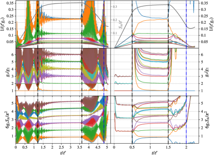
Figure 5: (color online). Time evolution of $(\ell g_{r})^{-1}$ (top), $g_{r}/g_{1}$ (middle) and $g_{r}S_{A}$ (bottom) after quenches such that $H$ and $H_{0}$ belong to different phases given by $\theta_{0}=\pi/8\to\theta=\pi/2-\pi/8$ (left) and $\theta_{0}=\pi/2-\pi/8\to\theta=\pi/8$ (right), for an interval having $\ell=128$ sites in the chain with PBC having $L=512$ sites.

Gapped evolution Hamiltonians.

It is very instructive to perform the numerical analysis of the ES discussed above for quenches where the post-quench Hamiltonian is gapped. In Fig. 5 we report the results obtained for a typical quench across the QCP, in both the directions. A major difference between the time evolutions of the ES after these two protocols is the occurrence of singularities in the regimes I and III for the quench from the paramagnetic phase to the ferromagnetic phase (left panels). In Torlai et al. (2014) it has been shown that the times at which the ES develops singularities in the regime I coincide with the times when the Loschmidt echo is singular, identifying the quantum dynamical phase transition Heyl et al. (2013) (see Heyl (2019) for a recent review).

In the quench from the ferromagnetic phase to the paramagnetic phase (right panels), the evolutions are smooth and, surprisingly, in the regimes I and II for the ratios $g_{r}/g_{1}$ we observe plateaux corresponding to integer values. It is remarkable that $g_{r}/g_{1}$ display plateaux at integer values in the time regime II also for the quench from the paramagnetic phase to the ferromagnetic phase. This feature, which has been highlighted for the quench at the QCP (see regime I in Fig. 2), could be attributed to the crossing of the QCP. Indeed, in Fig. 6, where the QCP is not crossed, these plateaux at integer values for $g_{r}/g_{1}$ in the regime II are not observed. The collapse of the curves on the integer values in the regime II of the quench from the paramagnetic phase to the ferromagnetic phase improves as $|\theta-\theta_{0}|$ increases. According to the discussion reported above for the quenches at the QCP, these integer values could be related to two copies of the Ising BCFT on the annulus with CBC $a$ and $b_{0}$, like the regime I of the quench at the QCP (see Fig. 2). Analytic results supporting this observation are missing. A possible interpretation could rely on the fact that, being the evolution Hamiltonian gapped, the correlation length is finite and therefore the entangling points can be considered independent from each other, as in the regime I of the quench at the QCP.

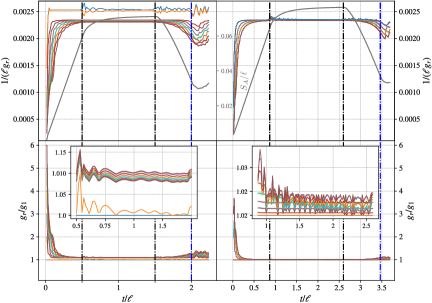
Figure 6: (color online). Time evolution of $(\ell g_{r})^{-1}$ (top) and $g_{r}/g_{1}$ (bottom) after the quench $\theta_{0}=\pi/12\to\theta=\pi/4-\pi/12$ within the paramagnetic phase (left) and $\theta_{0}=\pi/2-\pi/12\to\theta=\pi/4+\pi/12$ within the ferromagnetic phase (right), for an interval with $\ell=128$ sites in chain with PBC having $L=512$ sites.

Summary and discussion.

In finite TFIC with either PBC or OBC (reflecting boundaries), we have studied numerically the time evolution of the gaps $g_{r}$ of the ES after a global quantum quench of the magnetic field, when the subsystem is an interval. We found that interesting information is provided by the ratios $g_{r}/g_{1}$, which take constant values in various time regimes, for the lower part of the ES. In particular, when the post-quench Hamiltonian is critical, the first thermalisation regime (regime II) is determined by the conformal spectrum of the Ising BCFT on the annulus with the proper CBC. Surprisingly, this feature is observed also for quenches across the QCP. Furthermore, these results are robust under reasonable changes of the initial state. Our analysis leads to identify the proper CBC to adopt in the BCFT approach to global quenches of Calabrese and Cardy (2005, 2006, 2007); Cardy (2014, 2016); Cardy and Tonni (2016) that allow to reproduce the numerical results (as done in Läuchli (2013) at equilibrium in the ground state).

The numerical results reported here naturally require further investigations in many directions. Repeating our analysis for finite open TFIC with different boundary conditions would improve the current understanding of the role of the boundaries in the imaginary time path integral approach. It is worth extending our analysis to other spin chains (e.g. XXZ and the Hubbard model), both in the universality class of the TFIC and in different ones. Reproducing our results through GGE methods would be very insightful. The relation between the ES and the features of the dynamical quantum phase transitions deserves further, more quantitative, analysis. Interesting results about the ES could be obtained also by considering directly the entanglement Hamiltonian Bisognano and Wichmann (1975); Peschel and Chung (1999); Peschel (2003, 2004b); Peschel and Eisler (2009); Casini et al. (2011); Eisler and Peschel (2017); Eisler et al. (2019); Di Giulio et al. (2019); Fagotti and Essler (2013) or bipartitions where $A$ is made by disjoint intervals or spatially inhomogeneous lattice systems Tonni et al. (2018). It is instuctive to study the time evolution of the ES after local quantum quenches J. Surace et al. . Extending all these analysis to higher dimensions is also very important. Finally, we remark that our results naturally suggest that experiments on entanglement spectroscopy of out-of-equilibrium correlated many-body quantum systems could provide efficient methods to measure the critical exponents.

We are grateful to Giuseppe Di Giulio, Glen Evenbly, Andreas Ludwig, Giuseppe Mussardo, Anatoli Polkovnikov and Marcos Rigol for useful discussions and in particular to John Cardy for his comments on the draft. JS is supported by the doctoral training partnership (DTP 2016-2017) of the University of Strathclyde. LT is supported by the MINECO RYC-2016-20594 fellowship and the MINECO PGC2018-095862-B-C22 grant. We thank the organisers of the workshop Entangle This IV: Chaos, Order and Qubits (ICMAT, Madrid), where these results have been presented by LT. ET acknowledges Yukawa Institute for Theoretical Physics at Kyoto University, where part of this work has been done, during the workshop YITP-T-19-03 Quantum Information and String Theory 2019, and Trieste Institute for Theoretical Quantum Technologies.

References

- Hastings (2007) M. B. Hastings, J. Stat. Mech.: Theory Exp. 2007, P08024 (2007).
- Masanes (2009) L. Masanes, Phys. Rev. A 80, 052104 (2009).
- Amico et al. (2008) L. Amico, R. Fazio, A. Osterloh, and V. Vedral, Rev. Mod. Phys. 80, 517 (2008).
- Bridgeman and Chubb (2017) J. C. Bridgeman and C. T. Chubb, J. Phys. A: Math. Theor. 50, 223001 (2017).
- Orús (2014) R. Orús, Ann. Phys. (N. Y.) 349, 117 (2014).
- Ran et al. (2017) S.-J. Ran, E. Tirrito, C. Peng, X. Chen, L. Tagliacozzo, G. Su, and M. Lewenstein, (2017), arXiv:1708.09213 .
- Pelissetto and Vicari (2002) A. Pelissetto and E. Vicari, Phys. Rep. 368, 549 (2002).
- Belavin et al. (1984) A. A. Belavin, A. M. Polyakov, and A. B. Zamolodchikov, Nucl. Phys. B B241, 333 (1984).
- Henkel (1999) M. Henkel, Conformal Invariance and Critical Phenomena, Theoretical and Mathematical Physics (Springer-Verlag, Berlin Heidelberg, 1999).
- Holzhey et al. (1994) C. Holzhey, F. Larsen, and F. Wilczek, Nucl. Phys. B 424, 443 (1994).
- Calabrese and Cardy (2004) P. Calabrese and J. Cardy, J. Stat. Mech.: Theory Exp. 2004, P06002 (2004).
- Vidal et al. (2003) G. Vidal, J. I. Latorre, E. Rico, and A. Kitaev, Phys. Rev. Lett. 90, 227902 (2003).
- Callan and Wilczek (1994) C. Callan and F. Wilczek, Phys. Lett. B 333, 55 (1994).
- Calabrese et al. (2009) P. Calabrese, J. Cardy, and E. Tonni, J. Stat. Mech.: Theory Exp. 2009, P11001 (2009).
- Calabrese et al. (2011) P. Calabrese, J. Cardy, and E. Tonni, J. Stat. Mech.: Theory Exp. 2011, P01021 (2011).
- Alba et al. (2011) V. Alba, L. Tagliacozzo, and P. Calabrese, J. Stat. Mech.: Theory Exp. 2011, P06012 (2011).
- Coser et al. (2014a) A. Coser, L. Tagliacozzo, and E. Tonni, J. Stat. Mech.: Theory Exp. 2014, P01008 (2014a).
- De Nobili et al. (2015) C. De Nobili, A. Coser, and E. Tonni, J. Stat. Mech.: Theory Exp. 2015, P06021 (2015).
- Li and Haldane (2008) H. Li and F. D. M. Haldane, Phys. Rev. Lett. 101, 010504 (2008).
- Peschel and Truong (1987) I. Peschel and T. T. Truong, Z. Physik B 69, 385 (1987).
- Calabrese and Lefevre (2008) P. Calabrese and A. Lefevre, Phys. Rev. A 78, 032329 (2008).
- Poilblanc (2010) D. Poilblanc, Phys. Rev. Lett. 105, 077202 (2010).
- Cirac et al. (2011) J. I. Cirac, D. Poilblanc, N. Schuch, and F. Verstraete, Phys. Rev. B 83, 245134 (2011).
- Dubail et al. (2012) J. Dubail, N. Read, and E. H. Rezayi, Phys. Rev. B 85, 115321 (2012).
- Läuchli (2013) A. M. Läuchli, (2013), arXiv:1303.0741 .
- Cardy and Tonni (2016) J. Cardy and E. Tonni, J. Stat. Mech.: Theory Exp. 2016, 123103 (2016).
- Cardy (2011) J. Cardy, Phys. Rev. Lett. 106, 150404 (2011).
- Abanin and Demler (2012) D. A. Abanin and E. Demler, Phys. Rev. Lett. 109, 020504 (2012).
- Daley et al. (2012) A. J. Daley, H. Pichler, J. Schachenmayer, and P. Zoller, Phys. Rev. Lett. 109, 020505 (2012).
- Islam et al. (2015) R. Islam, R. Ma, P. M. Preiss, M. Eric Tai, A. Lukin, M. Rispoli, and M. Greiner, Nature 528, 77 (2015).
- Hauke et al. (2016) P. Hauke, M. Heyl, L. Tagliacozzo, and P. Zoller, Nat. Phys. 12, 778 (2016).
- Pichler et al. (2016) H. Pichler, G. Zhu, A. Seif, P. Zoller, and M. Hafezi, Phys. Rev. X 6, 041033 (2016).
- Kaufman et al. (2016) A. M. Kaufman, M. E. Tai, A. Lukin, M. Rispoli, R. Schittko, P. M. Preiss, and M. Greiner, Science 353, 794 (2016).
- Brydges et al. (2019) T. Brydges, A. Elben, P. Jurcevic, B. Vermersch, C. Maier, B. P. Lanyon, P. Zoller, R. Blatt, and C. F. Roos, Science 364, 260 (2019).
- Lukin et al. (2019) A. Lukin, M. Rispoli, R. Schittko, M. E. Tai, A. M. Kaufman, S. Choi, V. Khemani, J. Léonard, and M. Greiner, Science 364, 256 (2019).
- Calabrese and Cardy (2005) P. Calabrese and J. Cardy, J. Stat. Mech.: Theory Exp. 2005, P04010 (2005).
- De Chiara et al. (2006) G. De Chiara, S. Montangero, P. Calabrese, and R. Fazio, J. Stat. Mech.: Theory Exp. 2006, P03001 (2006).
- Coser et al. (2014b) A. Coser, E. Tonni, and P. Calabrese, J. Stat. Mech.: Theory Exp. 2014, P12017 (2014b).
- Nahum et al. (2017) A. Nahum, J. Ruhman, S. Vijay, and J. Haah, Phys. Rev. X 7, 031016 (2017).
- Vidal (2004) G. Vidal, Phys. Rev. Lett. 93, 040502 (2004).
- White and Feiguin (2004) S. R. White and A. E. Feiguin, Phys. Rev. Lett. 93, 076401 (2004).
- Daley et al. (2004) A. J. Daley, C. Kollath, U. Schollwöck, and G. Vidal, J. Stat. Mech.: Theory Exp. 2004, P04005 (2004).
- Paeckel et al. (2019) S. Paeckel, T. Köhler, A. Swoboda, S. R. Manmana, U. Schollwöck, and C. Hubig, (2019), arXiv:1901.05824 .
- Leviatan et al. (2017) E. Leviatan, F. Pollmann, J. H. Bardarson, D. A. Huse, and E. Altman, (2017), arXiv:1702.08894 .
- White et al. (2017) C. D. White, M. Zaletel, R. S. K. Mong, and G. Refael, (2017), arXiv:1707.01506 .
- Surace et al. (2019) J. Surace, M. Piani, and L. Tagliacozzo, Phys. Rev. B 99, 235115 (2019).
- Rams and Zwolak (2019) M. M. Rams and M. Zwolak, (2019), arXiv:1904.12793 .
- Krumnow et al. (2019) C. Krumnow, J. Eisert, and Ö. Legeza, (2019), arXiv:1904.11999 .
- Fausti et al. (2011) D. Fausti, R. I. Tobey, N. Dean, S. Kaiser, A. Dienst, M. C. Hoffmann, S. Pyon, T. Takayama, H. Takagi, and A. Cavalleri, Science 331, 189 (2011).
- Abanin and Papić (2017) D. A. Abanin and Z. Papić, Annalen der Physik 529, 1700169 (2017).
- Alet and Laflorencie (2018) F. Alet and N. Laflorencie, Comptes Rendus Physique 19, 498 (2018).
- Rigol et al. (2008) M. Rigol, V. Dunjko, and M. Olshanii, Nature 452, 854 (2008).
- Polkovnikov et al. (2011) A. Polkovnikov, K. Sengupta, A. Silva, and M. Vengalattore, Rev. Mod. Phys. 83, 863 (2011).
- Eisert et al. (2015) J. Eisert, M. Friesdorf, and C. Gogolin, Nat. Phys. 11, 124 (2015).
- D’Alessio et al. (2016) L. D’Alessio, Y. Kafri, A. Polkovnikov, and M. Rigol, Adv. Phys. 65, 239 (2016).
- Prüfer et al. (2018) M. Prüfer, P. Kunkel, H. Strobel, S. Lannig, D. Linnemann, C.-M. Schmied, J. Berges, T. Gasenzer, and M. K. Oberthaler, Nature 563, 217 (2018).
- Heyl et al. (2013) M. Heyl, A. Polkovnikov, and S. Kehrein, Phys. Rev. Lett. 110, 135704 (2013).
- Žunkovič et al. (2018) B. Žunkovič, M. Heyl, M. Knap, and A. Silva, Phys. Rev. Lett. 120, 130601 (2018).
- Heyl (2019) M. Heyl, EPL 125, 26001 (2019).
- Jordan and Wigner (1928) P. Jordan and E. Wigner, Z. Phys. 47, 631 (1928).
- Lieb et al. (1961) E. Lieb, T. Schultz, and D. Mattis, Ann. Phys. (N. Y.) 16, 407 (1961).
- Barouch et al. (1970) E. Barouch, B. M. McCoy, and M. Dresden, Phys. Rev. A 2, 1075 (1970).
- Barouch and McCoy (1971a) E. Barouch and B. M. McCoy, Phys. Rev. A 3, 786 (1971a).
- Barouch and McCoy (1971b) E. Barouch and B. M. McCoy, Phys. Rev. A 3, 2137 (1971b).
- Di Giulio et al. (2019) G. Di Giulio, R. Arias, and E. Tonni, (2019), arXiv:1905.01144 .
- Calabrese and Cardy (2006) P. Calabrese and J. Cardy, Phys. Rev. Lett. 96, 136801 (2006).
- Calabrese and Cardy (2007) P. Calabrese and J. Cardy, J. Stat. Mech.: Theory Exp. 2007, P06008 (2007).
- Robinson (1976) D. W. Robinson, The Journal of the Australian Mathematical Society. Series B. Applied Mathematics 19, 387 (1976).
- Bratteli and Robinson (1981) O. Bratteli and D. W. Robinson, Operator Algebras and Quantum Statistical Mechanics II: Equilibrium States Models in Quantum Statistical Mechanics, Theoretical and Mathematical Physics (Springer-Verlag, Berlin Heidelberg, 1981).
- Cardy (2014) J. Cardy, Phys. Rev. Lett. 112, 220401 (2014).
- Cardy (2016) J. Cardy, J. Phys. A: Math. Theor. 49, 415401 (2016).
- Takayanagi and Ugajin (2010) T. Takayanagi and T. Ugajin, J. High Energy Phys. 2010, 54 (2010).
- da Silva et al. (2015) E. da Silva, E. Lopez, J. Mas, and A. Serantes, J. High Energy Phys. 2015, 38 (2015).
- Rigol et al. (2006) M. Rigol, A. Muramatsu, and M. Olshanii, Phys. Rev. A 74, 053616 (2006).
- Rigol et al. (2007) M. Rigol, V. Dunjko, V. Yurovsky, and M. Olshanii, Phys. Rev. Lett. 98, 050405 (2007).
- Vidmar and Rigol (2016) L. Vidmar and M. Rigol, J. Stat. Mech.: Theory Exp. 2016, 64007 (2016).
- (77) J. Surace, L. Tagliacozzo, and E. Tonni, in preparation .
- Cardy (1986) J. Cardy, Nucl. Phys. B 275, 200 (1986).
- Cardy (1989) J. Cardy, Nucl. Phys. B 324, 581 (1989).
- Calabrese and Cardy (2016) P. Calabrese and J. Cardy, J. Stat. Mech.: Theory Exp. 2016, 064003 (2016).
- Peschel (2004a) I. Peschel, J. Stat. Mech.: Theory Exp. 2004, P06004 (2004a).
- Ohmori and Tachikawa (2015) K. Ohmori and Y. Tachikawa, J. Stat. Mech.: Theory Exp. 2015, P04010 (2015).
- Alba et al. (2017) V. Alba, P. Calabrese, and E. Tonni, J. Phys. A: Math. Theor. 51, 024001 (2017).
- Tonni et al. (2018) E. Tonni, J. Rodríguez-Laguna, and G. Sierra, J. Stat. Mech.: Theory Exp. 2018, 043105 (2018).
- Wen et al. (2018) X. Wen, S. Ryu, and A. W. W. Ludwig, J. Stat. Mech.: Theory Exp. 2018, 113103 (2018).
- Evenbly et al. (2010) G. Evenbly, R. N. C. Pfeifer, V. Picó, S. Iblisdir, L. Tagliacozzo, I. P. McCulloch, and G. Vidal, Phys. Rev. B 82, 161107 (2010).
- Evenbly and Vidal (2014) G. Evenbly and G. Vidal, J. Stat. Phys. 157, 931 (2014).
- (88) A. Polkovnikov and M. Rigol, private communication .
- Torlai et al. (2014) G. Torlai, L. Tagliacozzo, and G. De Chiara, J. Stat. Mech.: Theory Exp. 2014, P06001 (2014).
- Bisognano and Wichmann (1975) J. J. Bisognano and E. H. Wichmann, J. Math. Phys. 16, 985 (1975).
- Peschel and Chung (1999) I. Peschel and M.-C. Chung, J. Phys. A: Math. Gen. 32, 8419 (1999).
- Peschel (2003) I. Peschel, J. Phys. A: Math. Gen. 36, L205 (2003).
- Peschel (2004b) I. Peschel, J. Stat. Mech.: Theory Exp. 2004, P06004 (2004b).
- Peschel and Eisler (2009) I. Peschel and V. Eisler, J. Phys. A: Math. Theor. 42, 504003 (2009).
- Casini et al. (2011) H. Casini, M. Huerta, and R. C. Myers, J. High Energy Phys. 2011, 36 (2011).
- Eisler and Peschel (2017) V. Eisler and I. Peschel, J. Phys. A: Math. Theor. 50, 284003 (2017).
- Eisler et al. (2019) V. Eisler, E. Tonni, and I. Peschel, J. Stat. Mech.: Theory Exp. 2019, 073101 (2019).
- Fagotti and Essler (2013) M. Fagotti and F. H. L. Essler, Phys. Rev. B 87, 245107 (2013).