A Weighted -Minimization Approach For Wavelet Reconstruction of Signals and Images
Abstract
In this effort we propose a convex optimization approach based on weighted -regularization for reconstructing objects of interest, such as signals or images, that are sparse or compressible in a wavelet basis. We recover the wavelet coefficients associated to the functional representation of the object of interest by solving our proposed optimization problem. We give a specific choice of weights and show numerically that the chosen weights admit efficient recovery of objects of interest from either a set of sub-samples or a noisy version. Our method not only exploits sparsity but also helps promote a particular kind of structured sparsity often exhibited by many signals and images. Furthermore, we illustrate the effectiveness of the proposed convex optimization problem by providing numerical examples using both orthonormal wavelets and a frame of wavelets. We also provide an adaptive choice of weights which is a modification of the iteratively reweighted -minimization method introduced in [8].
I Introduction
We investigate recovering an object of interest (OoI) from either a small number of samples or a noisy version using a weighted -norm regularized convex optimization scheme with a specific choice of weights. Throughout this effort, the functional representation of an OoI is given by
| (1) |
where is in the domain of , and are two finite sets of multi-indices which we will specify later, is a family of scaling functions, is a family of wavelet functions, and is either a wavelet or scaling function coefficient. We will discuss the wavelet and scaling functions in Section II. The recovery of is achieved by identifying a vector of coefficients, , from our proposed convex optimization problem. The weighted -norm, is defined as
| (2) |
given the vector of weights where and the cardinality of is . The coefficients are obtained by solving
| (3) |
where is an -dimensional vector of evaluations of at the points which may or may not be noisy, is the scaled vector and is the matrix whose entries are
| (4) |
given the bijective mapping , evaluation points and . The parameter in (3) controls the trade off between the regularization of the solution enforced by the weighted -norm and the fidelity to the observation enforced by the -norm.
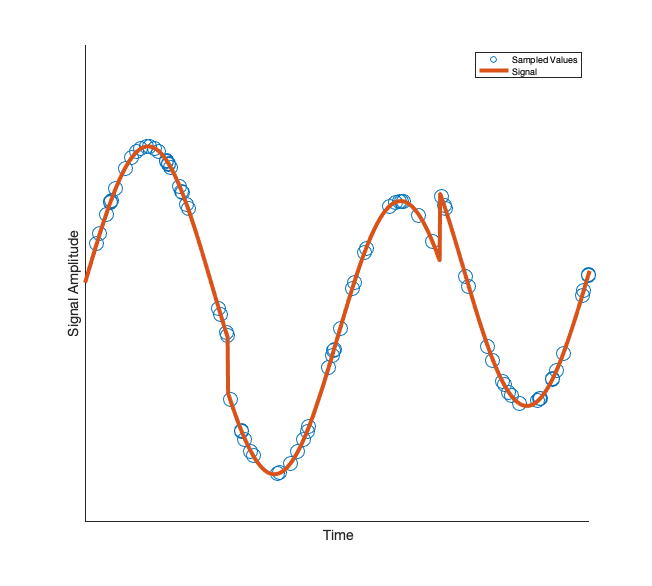
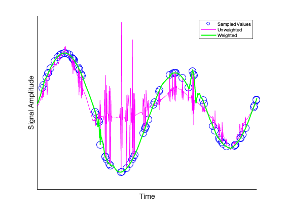
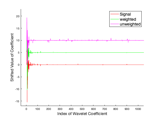
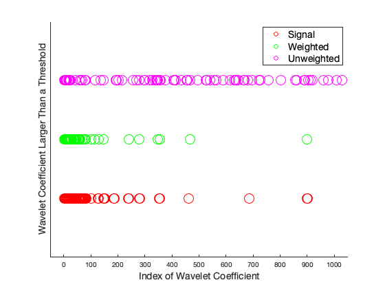
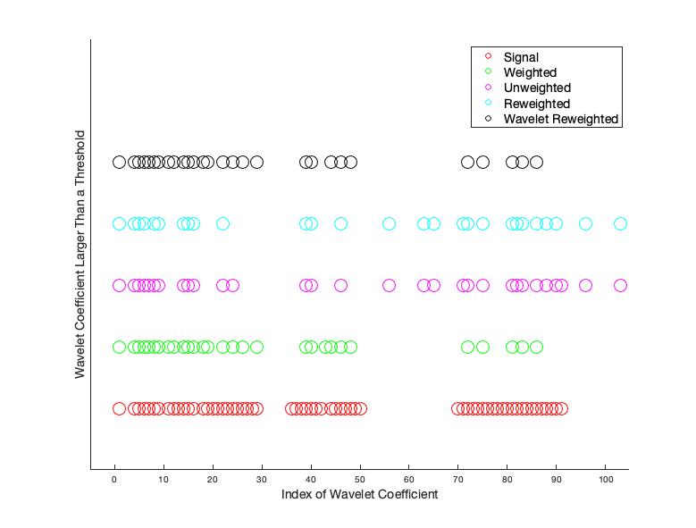
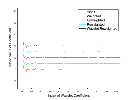
The effectiveness of -minimization is highlighted by its use in compressed sensing (CS) [7, 20] and has been successfully deployed in many applications such as photography [22], medical imaging [31] or radar and electromagnetic imaging [32]. Wavelet representations are extensively employed in data compression and denoising [21, 11]. Despite these triumphs, standard, unweighted -minimization, i.e., the minimization problem (3) where , does not seem suitable for the recovery of wavelet coefficients even for functions with sparse or compressible representations in a wavelet basis. Consider Figure 1(a) where a piecewise smooth function is plotted. As seen in Figure 2(a), many of its coefficients are relatively small (only out of the plotted coefficients have magnitude larger than ), so this function is compressible in wavelet basis. The indices of these large coefficients are given in Figure 2(b). From Figure 1(b) which plots the recovery of the piecewise smooth function from randomly chosen samples, it is readily seen that using unweighted -minimization is not satisfactory. Comparing the distribution of the large wavelet coefficients recovered by unweighted -minimization to those of the original signal, shown in Figure 2(a), it is clear that the unweighted approach leads to the recovery of spurious large coefficients that do not correspond to the true signal’s coefficients. Figure 2(b) shows the indices of the coefficients larger than the threshold recovered by unweighted -minimization. In particular, we notice that most of the large coefficients of the original signal are those with low indices, whereas the large coefficients recovered by unweighted -minimization are more uniformly distributed.
In this effort, we study a model for the structured sparsity of wavelet coefficients of OoI’s and consider several choices of weights chosen in a particular way which encourage that structure. We will use the weights
| (5) |
This choice is inspired by [12] where recovering the polynomial coefficients of high-dimensional functions by weighted -minimization is considered, and the indices of large polynomial coefficients of smooth functions typically fall in certain kinds of sets called “lower sets”. They show that using (5) vastly improves the recovery of the functions by proving that the recovered vector of coefficients has support which is very close to a lower set. In other words, the choice of weights promotes structure in the recovered coefficients. The same choice of weights, but definied with respect to wavelet functions in stead of polynomial ones, also promotes structure of wavelet coeffienits. Consider Figure 2(b) which compares the indices of the coefficients larger than the threshold for the original signal, those recovered by unweighted -minimization, and those recovered by weighted -minimization. Notice that the distribution of those coefficients recovered by weighted -minimization more closely resembles the distribution of the coefficients of the original signal. Furthermore, this choice of weights makes weighted -minimization robust in the sense that the recovered sparse vector is close to the true coefficients even when the measurements have been perturbed by noise. Our numerical examples in Section III show that weighted -minimization improves recovery for both inpainting and denoising, and encourages structured sparsity associated with wavelet coefficients. We also consider solving the inpainting problem using a frame of wavelets.
In this effort we also provide a choice of weights which can adapt to the structure of the wavelet coefficients of a given OoI. Since wavelets functions are scaled, shifted versions of a mother wavelet, the weights (5) depend only the scale of the associated coefficient. More complicated structures beyond the parent-child relationship may exist. That is, coefficients with large values are not randomly distributed within each scale. They may depend on other values within the same scale in addition to those on adjacent scales. Intuitively, improved performance can be obtained by choosing weights which are adapted to the inherent structure of a given set of wavelet coefficients both across and within scale. We consider a modification of iterative reweighted -minimization (IRW -minimization), introduced in [8], where a sequence of weighted -minimization problems are solved. The weights used in IRW -minimization are updated based on the previously recovered vector of coefficients. Our modification to IRW -minimization described in Section II updates the weights based on both the scale of the associated coefficients and the value of the coefficients recovered at the previous iteration. Our numerical examples which follow show that this adaptive choice of weights produces better results at the cost of solving several weighted -minimization problems.
I-A Related Results
Compressed Sensing based approaches for recovering a function from a limited collection of measurements or evaluations of a function were considered in [3, 6, 9, 23, 29, 34, 24] among others. Many of these works use the underlying assumption that the OoI can be well approximated by an expansion like (1) were only a few coefficients are large. Both the recovery of signals using weighted minimization and the use of structured sparsity have also been considered previously. For example, [36] studies a weighted approach and proposes some conditions for the weights, but does not provide a specific choice. An iterative process for choosing adaptive weights was introduced in [8] where weights are updated based on the coefficients recovered on the previous iteration. A specific choice of weights is given in [12] which yields a quantifiable improvement to the sample complexity. Binary weights are considered in [32]. A general class of structured sparse signals is considered in [3], where the authors establish a recovery guarantee with complexity estimates for two kinds of greedy algorithms. Another example where the structure of the wavelet trees is utilized is [6], where a novel, Gram-Schmidt process inspired implementation of an orthogonal matching pursuit algorithm is developed. The practicality of using sparse tree structures for real world signals has also been shown. The work [34] uses Compressed Sensing based recovery of the wavelet coefficients of electrocardiogram signals. Under certain structured sparsity assumption on the representation coefficients the authors in [1, 2] show that optimal sampling complexity can be achieved by unweighted -minimization if special sampling strategy is adopted. In particular this applies to the inpainting problem, however, in our case we assume that the samples are uniform and we do not have the freedom to choose the sampling strategy. Moreover, our structured assumption does not fit into their paradigm.
Exploiting the structure of wavelet coefficients has also been used to solve the denoising problem. Notice that noise added to the measurement principally contributes to the high frequency wavelet coefficients. Therefore, a naive wavelet denoising scheme is to take the wavelet transform of the noisy vector , threshold the wavelet coefficients and transform back into the original domain. By thresholding the wavelet coefficients we have removed some high frequency information from the wavelet coefficients and therefore we can expect that the some of the noise is also removed. More sophisticated thresholding methods have been considered, see e.g., [21, 19, 35, 26]. Whereas these works employ statistical estimation to find important wavelet coefficients, our work finds out that with a simple choice of weights which is independent of the OoI, we can obtain satisfactory denoising results. Our proposed weighted -minimization recovers a vector of coefficients which, due to our choice of weights, is less likely to be affected by the high-frequency perturbations in the function samples.
I-B Organization
In Section II we present our choices of weights and review the relevant research which influenced our approach. We also introduce a model for wavelet coefficients which futher supports our choice of weights.
In Section III, we present some numerical experiments which show that an OoI can be successfully recovered using (3) our specific choices of weights (5) and (15). In particular, we consider the recovery of signals, images, and hyperspectral images from a set of incomplete measurements. We also solve the denoising problem for signals and images.
In Section IV we discuss possible extensions of this work.
II Theoretical Discussion
In this section we discuss several theoretical elements, which inspired our choice of weights, that we claim to promote the natural structure exhibited by the important wavelet coefficients of real-world OoI. Before justifying this claim and presenting a model for wavelet coefficients, we will first define -ary trees, which are a special case of a kind of graph called a tree. A directed graph is called a tree if it satisfies the following two conditions: (i) there is a single node, , which is called the root; and, (ii) there exists one and only one path from to any other node in the graph [25]. The indices of the wavelet coefficients can be identified with a node on a full -ary tree, i.e., a tree so that every node has either edges or zero edges leaving it. For example, Figure 3(a) shows an example of a -tree with the indices . In our model, the edges between nodes are directed and the direction determines a parent-child relationship between nodes. We say that node is the parent of node , or equivalently, the node is the child of node if one of the edges emanating from terminates at node . In general, we denote the parent of node as . To illustrate, consider Figure 3(a) where has two child nodes, and , so that . We consider the closed tree model for describing the subsets of large coefficients of signals and images.
Definition 1 (Closed Tree).
A multi-index set is called a closed tree if the following two conditions hold:
-
1.
Each may be uniquely identified with a node on a -ary tree.
-
2.
For each node ,
That is, if a node is in , then so is its parent.


An example of a closed tree is given in Figure 3(b). The motivation for considering closed trees as a model for wavelet coefficients is three-fold.
-
•
One can construct orthogonal wavelets from a set of the nested approximation spaces called multi-resolution analyses that satisfy certain properties, see for example [27]. The nested relationship between these induces an association between certain wavelet functions on adjacent levels. With appropriate indexing of wavelet function, the parent and child relationship of the closed tree corresponds to this association.
-
•
The coefficients of a function expressed in an orthonomral wavelet system are given by the inner product of the function with a wavelet function. In practice, this value is approximated using a quadrature rule. This quadrature can be implemented as a linear combination of scaling function coefficients at the previous scale [17]. Calculating coefficients in this way clear associates the value of the coefficient associated with a parent to the coefficients associated with its child nodes.
- •
This model makes rigorous a widely known property of wavelet representation of signals and images that nodes associated with small wavelet coefficients are more likely to have small children and nodes associated with large wavelet coefficients may have either large or small children. In light of this it is natural to find a choice of weights which promotes this structure. Our choice of weights is inspired by [12] where it was proven that polynomial coefficients that are associated with certain kinds of subsets, called lower sets, can be recovered with weighted -minimization with weights equal to the uniform norms of the tensor product polynomials associated with the coefficients.
Definition 2 (lower set).
A multi-index set is called a lower set if and only if
where is interpreted as for each .
Closed trees have analogous structure to lower sets in the sense that the parent of every node in the closed tree is also in the closed tree. Given a family of pre-defined wavelets, such as Haar, Daubechies, etc., the weight given in (5) is
| (6) |
where the multi-index and is the level on which the coefficients lies. In this section we established a structured sparsity model for wavelet coefficients and related wavelet and tensor product polynomial representations. In the next section we consider using weighted to recover a signal from incomplete or noisy measurements and justify our approach using these connections.
II-A Recovery of OoI from incomplete measurements
The minimum number of measurements required for the guaranteed recovery of a sparse vector is sometimes called the sampling complexity in the compressed sensing literature. For a measurement scheme arising from a bounded, orthonormal system, as in (4), the number of samples required for recovery using unweighted -minimization depends on the maximum of the uniform norms of the orthonormal system [24]. That is, let
| (7) |
then whenever satisfies
| (8) |
one can recover the best s-term approximation to the target function, i.e., an approximation formed by superimposing the functions from the orthonormal system corresponding to the largest coefficients. This condition is sharp or optimal for many sparse recovery problems of interest, for example, from Fourier measurements. However, for wavelets and high-dimensional polynomials, can become so large that renders (8) useless, see [37]. Motivated by the need of improved algorithms which can exploit the structure of sparse polynomial expansions with better recovery guarantee, [12] proposes a weighted approach where the sampling complexity depends on a quantity which is strictly smaller than . More rigorously, they showed that
| (9) |
where
| (10) |
is sufficient for the recovery of best term approximations with lower set structures. Assuming that an OoI has large wavelet coefficients lying on a closed tree, a similar conclusion about the sampling complexity of weighted -minimization (3) and (5) can be made. Let us define the analogous quantity to (10) for wavelets
| (11) |
Then it can be shown that the recovery guarantee is
| (12) |
and that,
| (13) |
so the sufficient condition on sampling complexity is improved.
Unlike the polynomial bases considered in [12], the guarantee (12) for wavelet bases is still too demanding. Moreover, it does not reflect the successful recovery from underdetermined systems, which is the main objective of a compressed sensing approach. We postulate that this is due to the limitation of our current analysis technique, and plan to address this issue in future work. In experiments, some shown in the following sections, we consistently observe that weighted -minimization is able to reconstruct signals and images given a small percentage of pixels. Therefore, (12) may be very pessimistic. More remarkably, the superiority of our proposed weighted -minimization approach over the unweighted approach is clear. In fact, our numerical examples show that it performs much better not only for orthonormal systems of wavelets but also for a frame wavelets which we introduce in Section III.
II-B Recovery of OoI from noisy measurements
Suppose that the samples used for the recovery of a function using (3) are noisy. In particular, we assume that where is modeled as a Gaussian noise. The denoising problem is to recover given . This can be solved by using our proposed weighted -minimization problem to recover the true coefficients of . In Section III, we give numerical examples of denoising full, noisy signals and images, i.e., . As mentioned in the introduction, a basic denoising approach is to threshold the wavelet coefficients of the noisy signal or image. This simple approach is effective if the noise level is small. For larger noise levels, more advanced thresholding algorithms have been proposed which adapt to the signal itself, for example, [21]. Our proposed weighted -minimization problem can be related to an iterative weighted soft-thresholding approach, where our choice of weights encourages the recovered wavelet coefficients to exhibit structure similar to the original signal. According to (6), the deeper a wavelet coefficient lies in the tree, the larger the weight associated with it is, resulting in more aggressive thresholding.
II-C Scale and Wavelet Aware Iteratively Updated Weights
Our choice of weights (5) naturally encourages the property that wavelet coefficients of different scales have appropriately scaled values. A natural extension would be to pick weights which take into account the intra-level magnitude correlation of coefficients. Although the true wavelet coefficients of an OoI have large and small values within each scale, our chosen weights do not discriminate between large and small coefficients within each scale. A method introduced in [8] iteratively solves several weighted -minimizations and updates the weights at each iteration based on the recovered sparse vector, specifically,
| (14) |
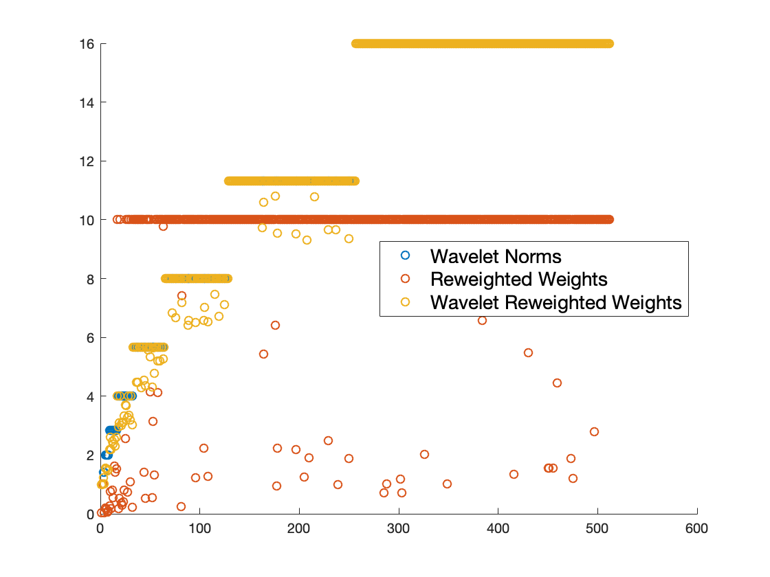
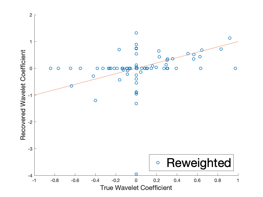
where is the coefficient recovered at step and is a parameter that must be chosen. Intuitively, this approach tries to find and minimize a concave penalty function that more closely resembles minimization. In practice however, this weighting strategy does not lead to significantly better results for recovering wavelet coefficients. In Figure 4, we see that similarly to the unweighted -minimization case, reweighted -minimization over emphasizes coefficients very deep in the wavelet tree leading to poor recovery. We recreated the results from the paper using the parameters provided by the authors.
From (6), it is clear that our choice of weights (5) depend on their level only. On the other hand, notice that the adaptive choice of weights used in the usual IRW -minimization does not take into account the level of the coefficients. We propose an alteration of IRW -minimization, where the weights are updated by the formula
| (15) |
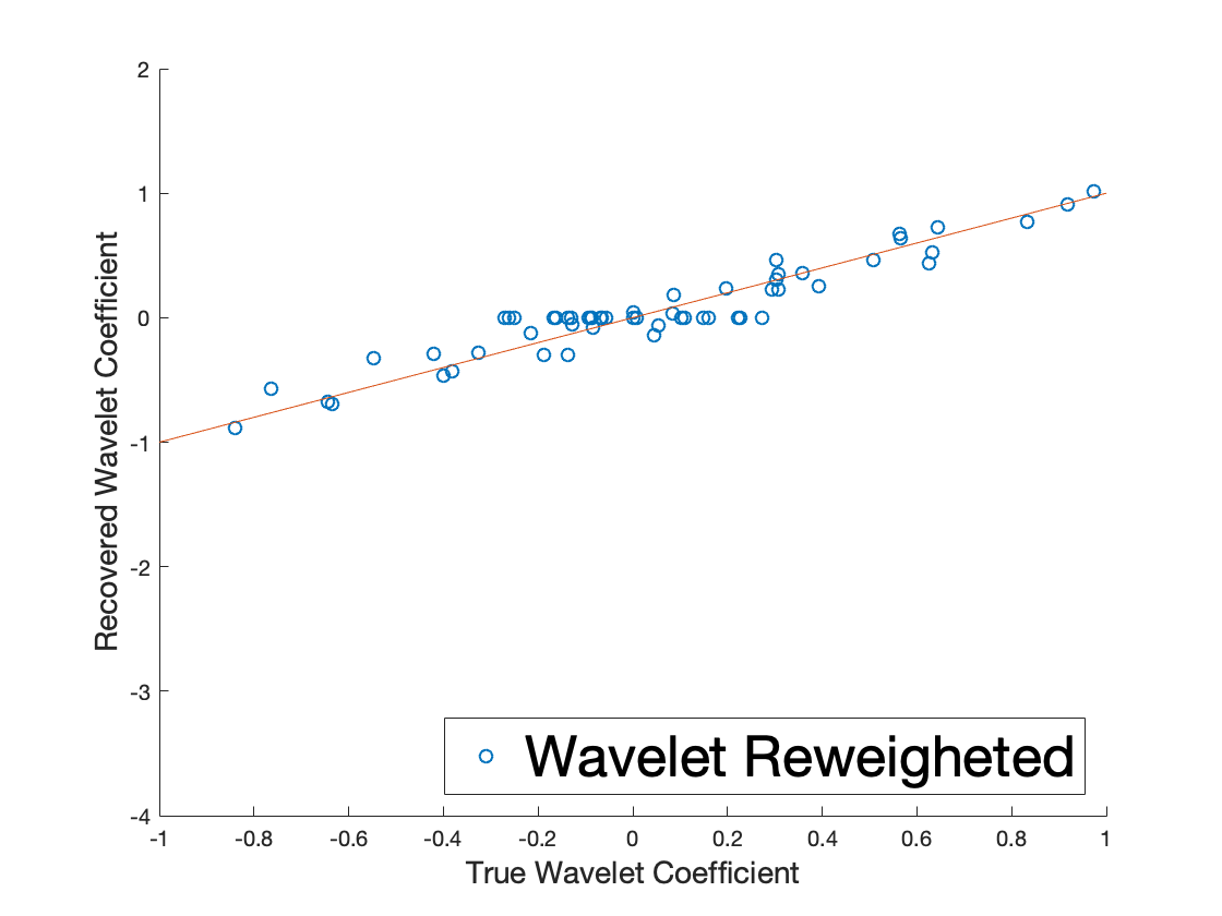
where is the weight from (5) and . Observe that the parent of each node is on a shallower level, which implies that , hence . The update (15) takes into account both the scale and specific choice of wavelet function and can be called scale and wavelet aware iteratively reweighted -minimization (hereafter referred to as wavelet reweighted -minimization).
The motivation for the updates used in wavelet reweighted are twofold. First, on the first iteration, the weights (15) are the same as (5), and therefore, they similarly encourage wavelet structured sparsity across levels. On later iterations, by (15), , hence the relative scales of recovered coefficients are maintained. Second, the term ensures that large coefficients have smaller weights than their sibling coeffients on the same scale. Our numerical examples show that the adaptive choice of weights (15) can perform somewhat better than the choice of weights (5), but at the cost of having to solve several weighted -minimization problems. We also see that it consistently performs much better than the usual IRW -minimization.
III Numerical experiments
In this section, we provide numerical results which show the effectiveness of weighted -minimization with our choice of weights for the recovery of the wavelet representations of signals, images and hyperspectral images. We also consider the weights
| (16) |
Our experiements indicate that choosing consistently performs well, where as choosing consistently performs poorly. There is not much difference in choosing , therefore the choice seems to be sufficient in general. We additionally present examples related to a frame of wavelets for use in the recovery of a signal from partial measurements as well as experiments using our adaptive choice of weights (15). Recovery of a functional representation of an OoI (1) is achieved by identifying the coefficients which minimize (3), then applying an inverse discrete wavelet transform to . The recovered signals and images presented below were obtained using SPGL1 [38, 39] for both the unweighted and the weighted cases. The wavelet transforms used are from the built-in MATLAB wavelet toolbox.
III-A Recovery of synthetic data compressible in wavelet basis
In this section we consider a synthetic example where the wavelet coefficients of a signal are exactly supported on a closed tree. We construct such a signal by randomly choosing a closed wavelet tree with nodes which is a sub-tree of a full binary tree with nodes. The coefficient values of these nodes are randomly assigned according to a Gaussian distribution whose mean and variance depend on the depth on the node. We reconstruct the signal using an inverse wavelet transform and randomly sample this signal at locations. These samples are used to recover coefficients using (3) with several choices of weights, IRW -minimization, and our wavelet reweighted -minimization. Our numerical experiments indicate that
-
•
the weighted approach outperforms the unweighted approach,
-
•
the success of weighted -minimization does not depend too heavily on the choice of , and
-
•
our wavelet reweighted approach slightly improves recovery.
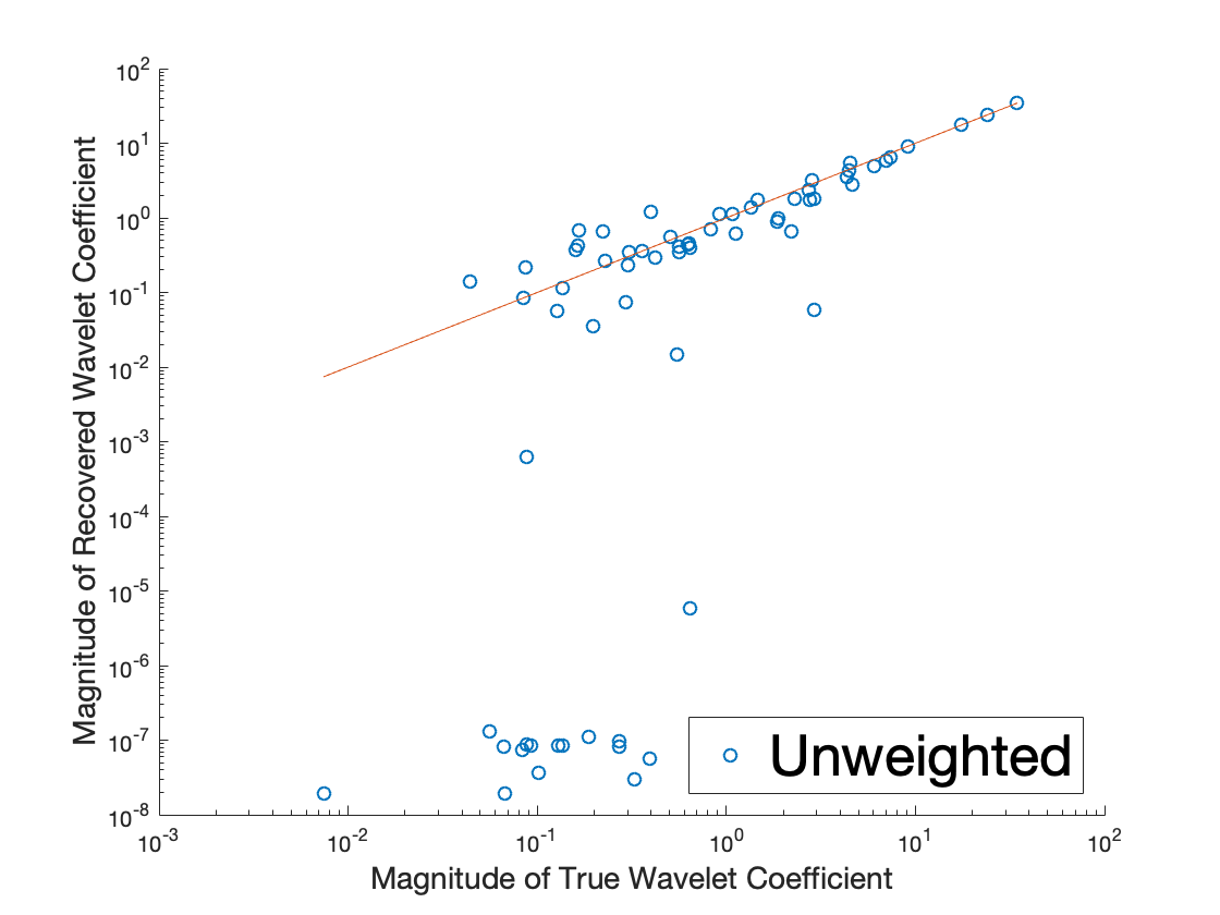
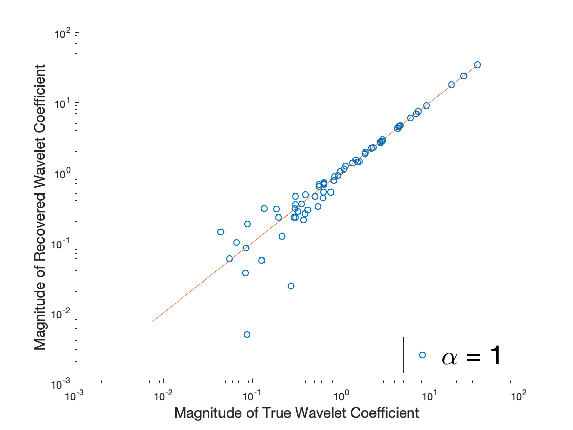
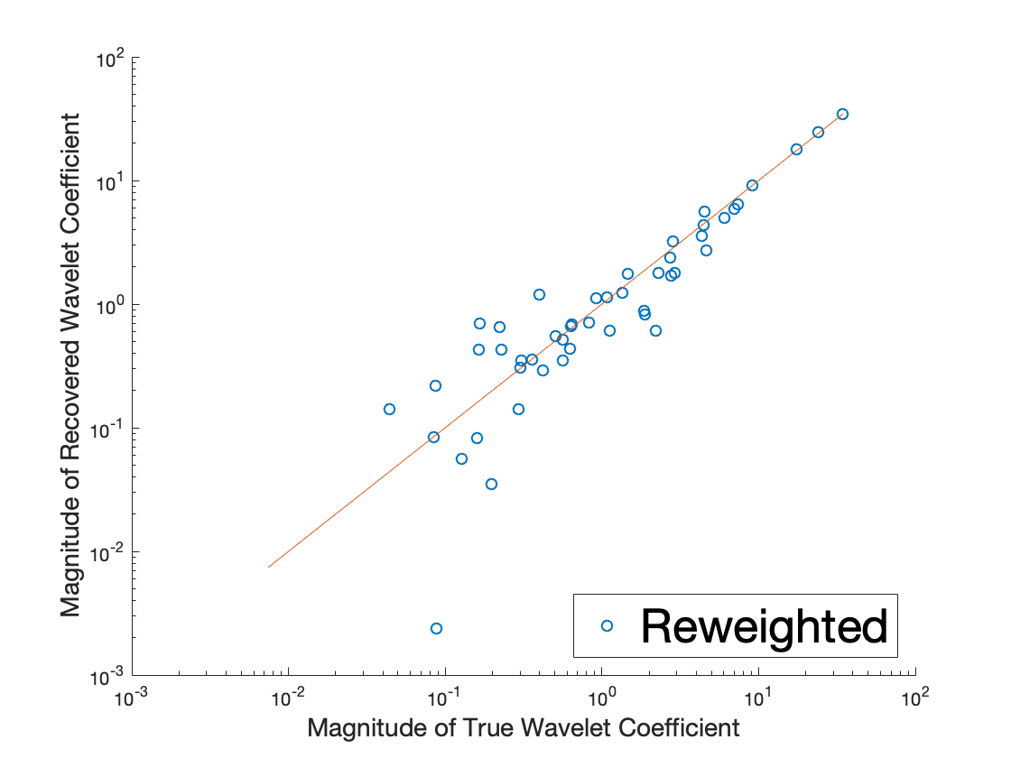
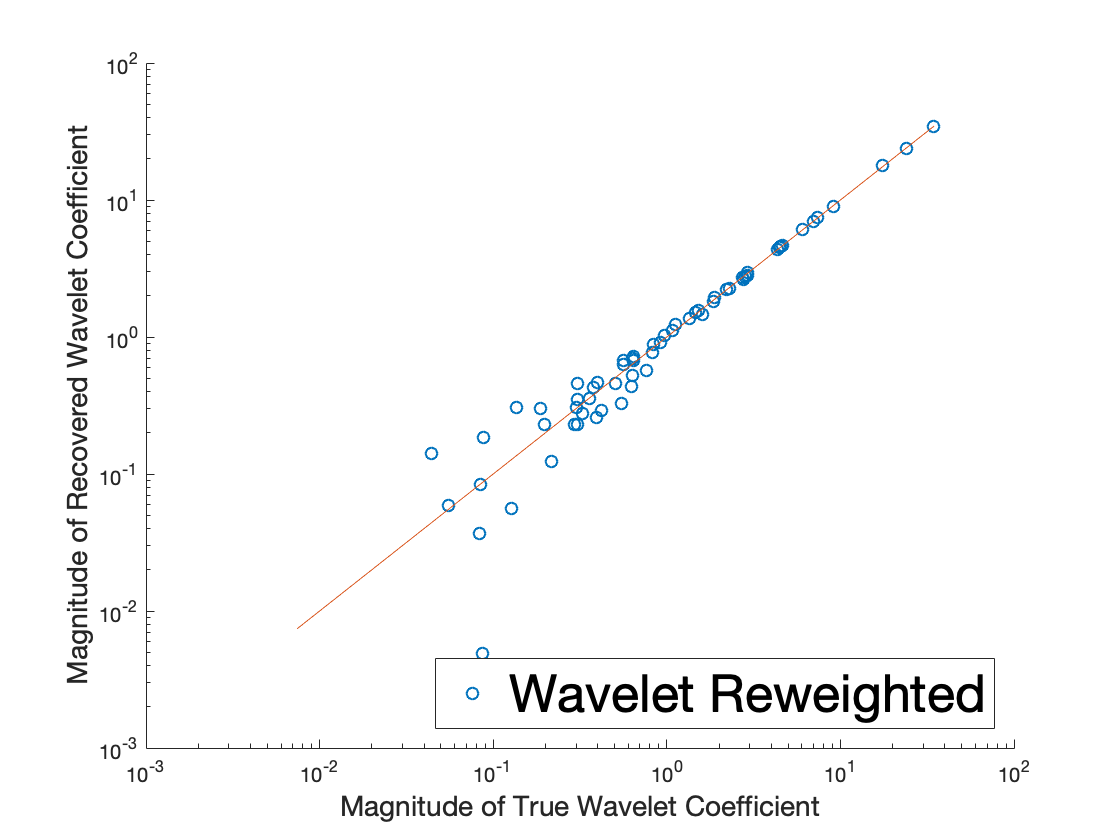
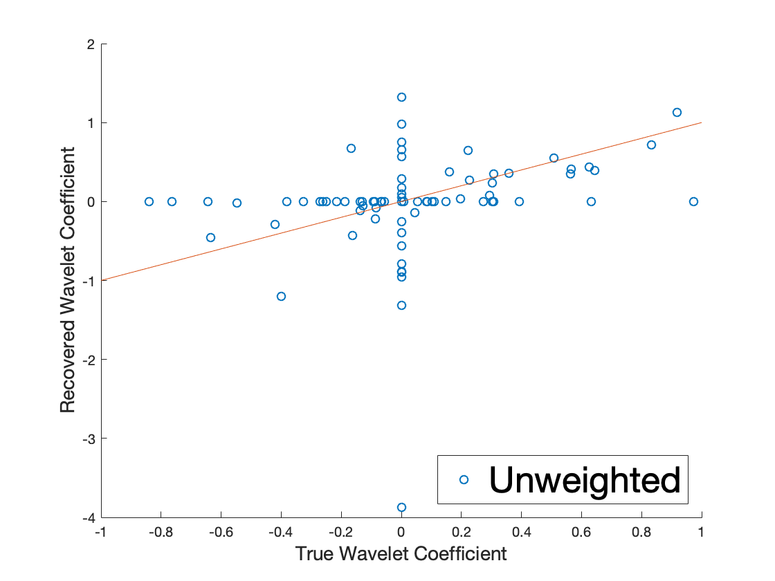
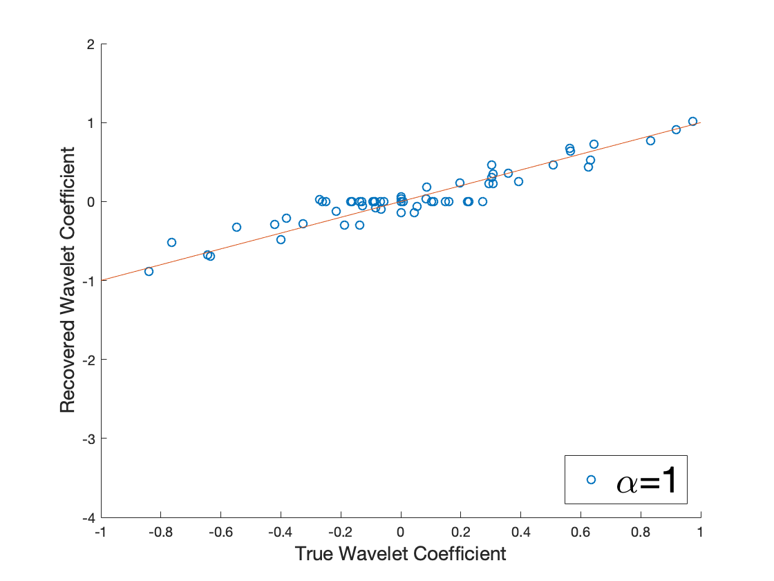
Figure 6 and Figure 7 compare the recovery of a randomly generated closed tree with nodes which is a subtree of wavelet tree with total nodes using weighted and unweighted -minimization. In each of the Figures, the recovered coefficients are associated with the vertical axis and the true coefficients are associated with the horizontal axis. If exact recovery is achieved then the points should all lie on the red line. Using a random sample of evaluations, we see that unweighted, weighted with , and reweighted -minimization identifies the significant coefficents. This can be seen in Figure 6, where the magnitudes of the recovered coefficients are plotted. Notice that the weighted approach is better able to capture the small coefficients. This is highlighted by Figure 7 where we plot the recovered coefficients against the true coefficietns in the interval .
Real-world signals and images do not possess wavelet coefficients which are exactly sparse and the large coefficients are unlikely exactly closed trees. Rather, they are often compressible in a wavelet basis. In this section we show that signals and images can be recovered from a relatively small number of measurements using weighted -minimization for the specific choice of weights (16). Our numerical experiments show that for , weighted -minimization far outperforms both unweighted -minimization and the usual reweighted -minimization.
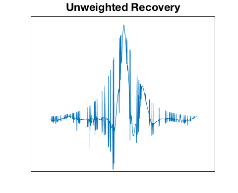
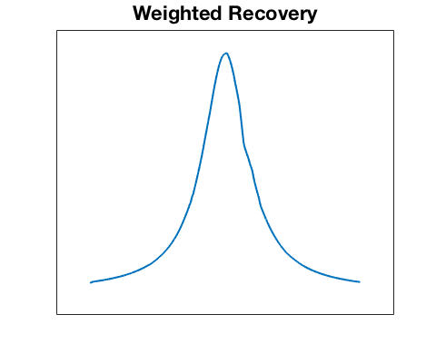
Figure 8 compares the recovery of the function from uniformly subsampled points chosen in the interval for different values of from (16) as well as unweighted and reweighted -minimization. The chosen wavelets are the one-dimensional coiflets constructed in [18]. The black dots in Figure 8(a) are the sampling points used in the reconstruction. Notice that the function recovered by our weighted approach is better than the one obtained using the unweighted approach. To quantify this, we calculated the Root-mean-square-error (RMSE) in each case. The unweighted case produced an RMSE of where as the the weighted case produced an RMSE of .
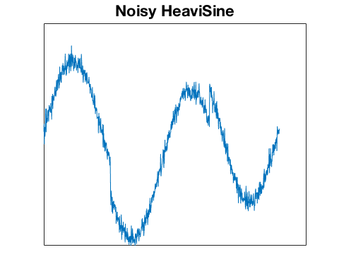
We compare two denoising schemes in Figure 9. A Gaussian noise was added to the piecewise smooth function as shown in Figure 9(a) so that the PSNR between the original Heavisine function and the noisy one is . Figure 9(b) shows the reconstruction using the built-in MATLAB function wden which automatically denoises using the adaptive wavelet shrinkage of the work [21]. This produces a reconstruction with PSNR . Figure 9(c) shows the reconstruction using our proposed weighted -minimization scheme and the PSNR is . While the built-in MATLAB function wden yields a reconstruction with better PSNR, notice that our reconstruction is more faithful to the features of the original signal and does not exhibit the extraneous fluctuations seen in Figure 9(b).


III-B Recovery of Images
In this section we consider the problem of reconstructing images from a small percentage of its pixels. In the RGB color model, the pixels of images are associated with 3-tuple describing a color. Images may be recovered by solving the multiple measurement vectors (MMV) version of weighted -minimization, i.e., we solve
| (17) |
where is a mixed norm defined as the weighted sum of the -norms of the rows of the matrix , is a matrix whose columns are the normalized observations of along each color band and where is the Frobenius norm.
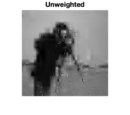
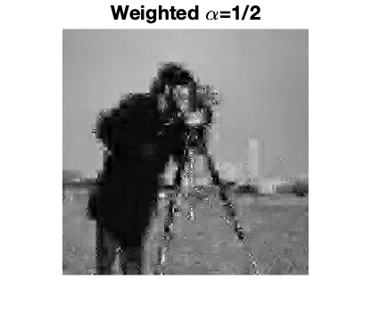
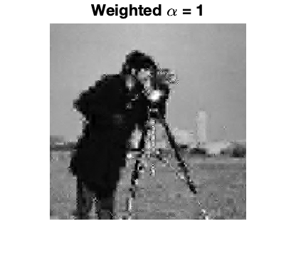
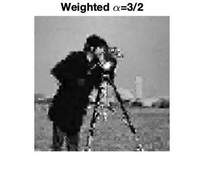
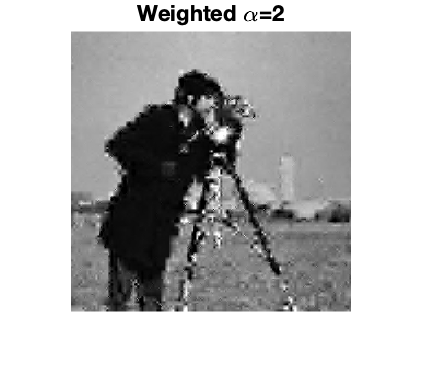
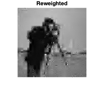
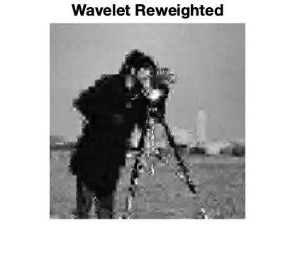
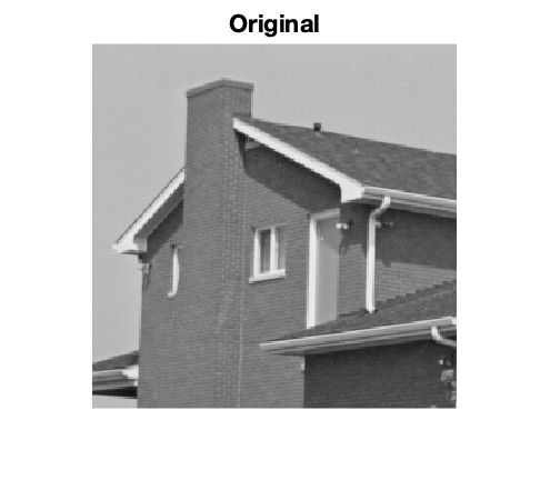
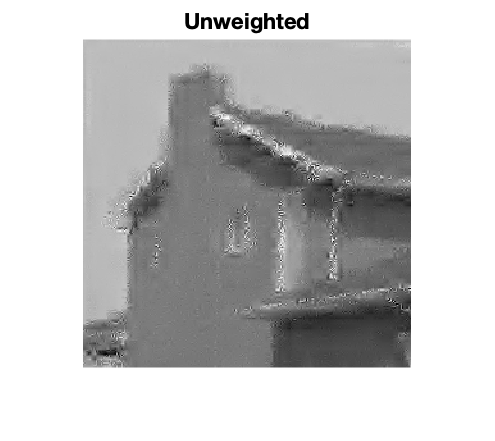
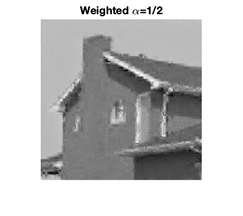
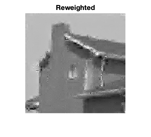
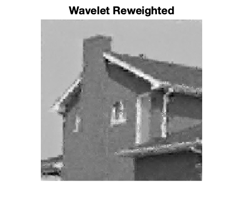
Figure 11 shows the recovery of a greyscale house image using several choices of . The original image has pixels and can be represented in the Haar wavelet basis with coefficeints. The measurements, , are randomly chosen pixels of the image so that , that is, the measurements are of the pixels, randomly chosen. Notice that the cases when vastly out perform IRW -minimization and unweighted -minimization. However, the differences between , , and are minimial. Therefore, choosing the weights as (5) is a reasonable choice in a general situation.
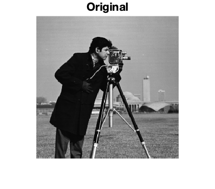


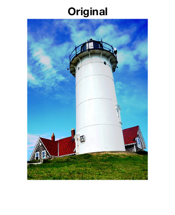
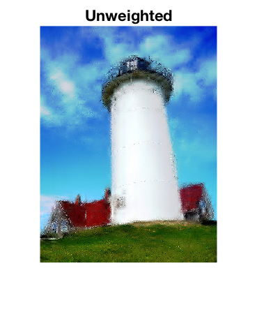
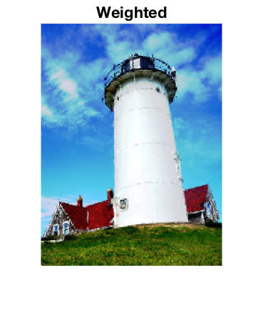
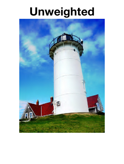
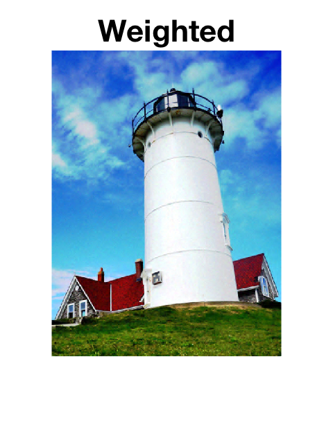
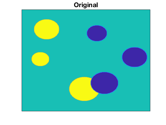
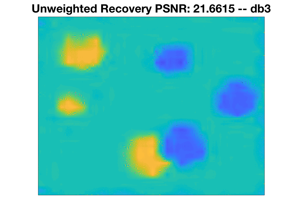
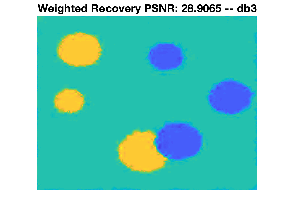
We can also recover color images by solving the minimization problem (17). Figure 12 shows that the weighted approach performs better than unweighted for color images. The PSNR of the reconstruction using unweighted -minimization is , see Figure 12(b). On the other hand, the PSNR using weighted -minimization is , see Figure 12(c). Notice that the unweighted recovery features blurring of edges and does not recover the texture of either the grass or the red roof tile. The weighted recovery exhibits a better recovery of sharp edges and the texture of the grass with yellow flowers. Weighted -minimization can also be deployed to recover other kinds of images besides the “natural landscape” type images typified by the lighthouse. Below we consider recovering cartoons, textures, and scientific data.
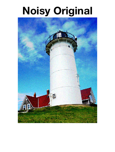
We also present an example of image denoising. Figure 13(a) is a noisy image generated by adding a Gaussian noise so that the PSNR of the noisy version is 26.0184. The reconstruction obtained using unweighted -minimization has PSNR , see Figure 13(b), and the weighted -minimization reconstruction has a PSNR , see Figure 13(c).
III-C Recovering Hyperspectral Images
The pixels of the color images we recovered in the previous section can be viewed as -tuples of numbers which represent the color at each pixel. The image itself can then be viewed as an object in where is the number of pixel along the width and is the number of pixels along the length. A hyperspectral image is an object in for some where and are the spatial dimensions and is the number of spectral bands. One can use the information stored in a hyperspectral image in a variety of contexts. Frequently, hyperspectral images are used for the remote detection or classification [10]. In particular, it has been used in medicine [30] for detection and classification of disease, and geology [40] for detection and classification of minerals or oil.
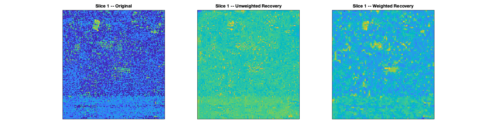
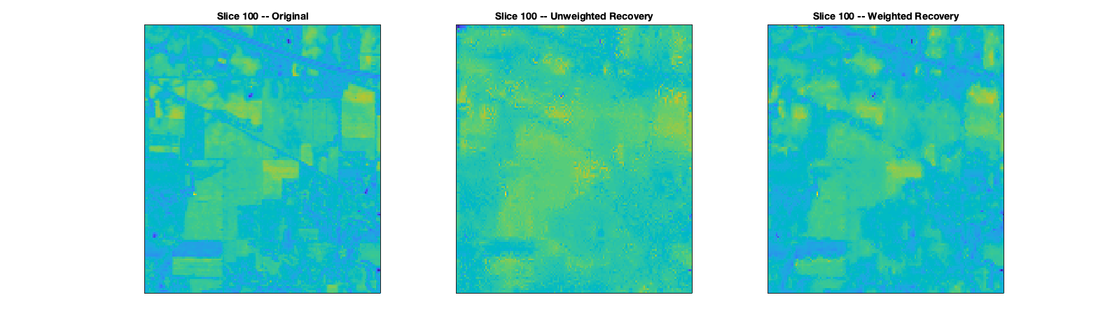
In our numerical experiment, we consider recovering a hyperspectral image from a set of subsampled spectral profiles at randomly chosen locations. In other words, we sample vectors from the hyperspectral image and wish to recover the full tensor. We do this by solving (17). For our experiment we have used a hyperspectral image associated with a natural landscape of fields. The spectrum at each pixel corresponds to the presense of certain wavelengths of light. For a sample of the spectral profiles at of the pixels we recover the tensor using weighted and unweighted -minimization.
In Figure 14 and Figure 15 we compare recovered slices of the tensor at spectral index and spectral index respectively. Notice that the unweighted approach does not yield as good results as the weighted approach.
For a particular pixel we can compare the recovery by looking at the spectral profile associated with that pixel. The spectral profile for the pixel and the recovered versions are plotted in Figure 16.

III-D Haar Framelets
Many successful image processing methods incorporate both local and global information about a signal to increase performance [4, 5, 28, 33]. In this section we consider a specific case of a representation system introduced in [41] where the simultaneous local and global feature analysis of an OoI is performed by a dictionary called a framelet. A sparse representation in the framelet dictionary recovered from a subsample set of measurements using our proposed weighted -minimization problem. The dictionary is constructed by taking the convolution of so called “local” and “global” bases discussed in more detail below.
Let be the vector representing the target digital signal. Local information is gathered by grouping neighboring evaluations around every point together into an array called a patch. For each , , the patch of length at location is defined where is interpreted as circular addition, i.e. is identified with , is identified with and so on. The patch matrix is constructed by setting the vector as the row of . Notice that has rows, one for each value in , and columns corresponding to the patch size.
The global basis is given as a matrix with its columns forming an orthonormal basis in , and the local basis is given as a matrix with its columns forming an orthonormal basis in . The patch matrix can be represented in the tensor product basis genereated from and with the coefficients computed by
| (18) |
The entries of the matrix can also be viewed as coefficients of in the convolutional framelet formed by the columns of and .
Definition 3 (Discrete, Circular Convolution).
For two vectors of length we define the discrete, circular convolution as an operator which returns a length vector whose component is
| (19) |
Let be the column of the matrix and be the column of . Denote by the vector whose first entries are identical with corresponding entries in , and the rest are equal to . The convolutional framelets are constructed as the circular convolution of with :
| (20) |
The vectors form a Parseval frame in (see [14] for definitions). The coefficients from (18) satisfy
and the vector can be recovered by the reconstruction formula
| (21) |
We choose the Haar basis for both the global and local basis in our numerical example. Consequently, for the the weights we have
| (22) |
where is the depth of the node associated with the wavelet function whose discretization is the row of and where is defined similarly for the Haar basis associated with .
In Figure 17 each of the reconstructions was created from 80 samples of a piecewise smooth function. Since the function is piecewise smooth, it is not necessary compressible in the Haar basis. The reconstructions using weighted and unweighted -minimization with the orthonormal Haar basis show “step”-like artifacts. On the other hand, the recovered framelet representation does not exhibit the step-like affects. Heuristically, the observed improved performance may be explained by the property that Haar framelets use local and global information simultaneously.


IV Conclusion
This effort has shown that weighted -minimization is effective for solving the interpolation/inpainting and denoising problems by recovering wavelet coefficients. Moreover, this effort provides two explicit choices for weights that do not require the identification of parameters beyond the choice of a wavelet family for use as a representation system. Provided numerical examples indicate that the choice of weights (5) far outperforms unweighted -minimization for recovering wavelet coefficients and that there is little difference between the case when and for the weights (16), hence, is a good choice. According to Figure 5, the weights used in IRW -minimization are not scaled appropriately. Our choice of weights (15) both iteratively updates weights so that large coefficients have smaller associated weights and ensures that the updated weights do not become too small. We also show that weighted -minimization can be used for measurement systems that do not happen to be an orthonormal system, see Section III-D. We have a proof which shows that the sampling complexity for our weighted -minimization is no worse than the sampling complexity for unweighted -minimization assuming that the sparse signal satisfies the closed tree assumption. In future work, it would be interesting to establish sharp estimates associated with wavelet based measurement systems. Such a result would theoretically explain the gap in performance between unweighted and weighted -minimizations for recovering wavelet coefficients. In this work we mainly consider images and signals. Another interesting direction to pursue would be to apply our choice of weights for recovering wavelet coefficients of functions which are solutions to partial differential equations.
Acknowledgements
This material is based upon work supported in part by: the U.S. Department of Energy, Office of Science, Early Career Research Program under award number ERKJ314; U.S. Department of Energy, Office of Advanced Scientific Computing Research under award numbers ERKJ331 and ERKJ345; the National Science Foundation, Division of Mathematical Sciences, Computational Mathematics program under contract number DMS1620280; Scientific Discovery through Advanced Computing (SciDAC) program through the FASTMath Institute under Contract No. DE-AC02-05CH11231; and by the Laboratory Directed Research and Development program at the Oak Ridge National Laboratory, which is operated by UT-Battelle, LLC., for the U.S. Department of Energy under contract DE-AC05-00OR22725.
-A Additional Numerical Examples
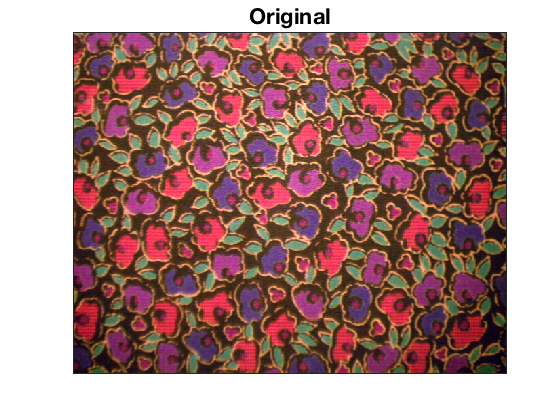
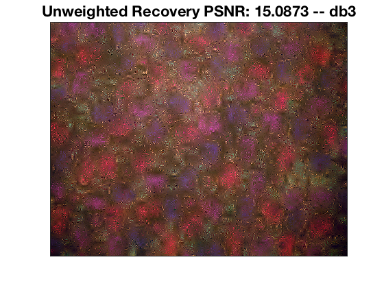
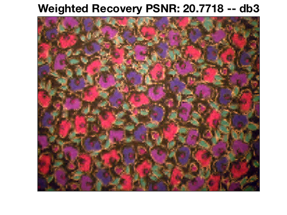
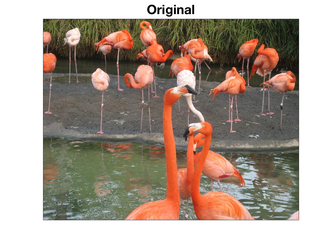
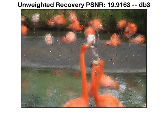
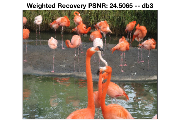
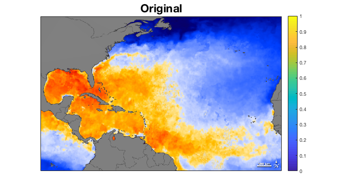
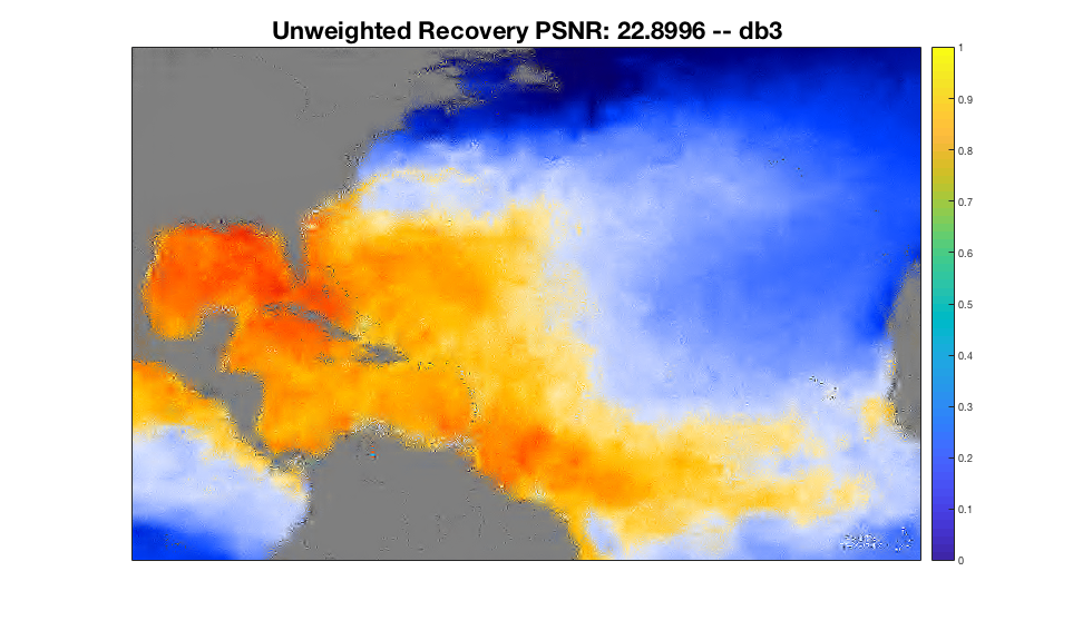
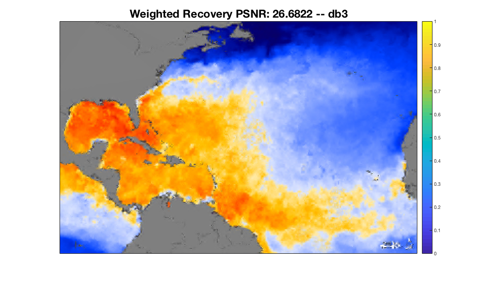
Here we consider more color examples for a variety of image types, namely, cartoons in Figure 18, textures in Figure 19, natural scenes with animals in Figure 20, and images genereated from scientific data in Figure 21.
References
- [1] Ben A., C. Boyer, and S. Brugiapaglia. On oracle-type local recovery guarantees in compressed sensing, 2018.
- [2] B. Adcock, A. C Hansen, C. Poon, and B. Roman. Breaking the coherence barrier: A new theory for compressed sensing. Forum of Mathematics, Sigma, 5, 2017.
- [3] R. G. Baraniuk, V. Cevher, M. F. Duarte, and Ch. Hegde. Model-based compressive sensing. IEEE Trans. Inform. Theory, 56(4):1982–2001, 2010.
- [4] A. Buades, B. Coll, and J. Morel. Non-Local Means Denoising. Image Processing On Line, 1:208–212, 2011.
- [5] A. Buades, B. Coll, and J. M. Morel. A review of image denoising algorithms, with a new one. Multiscale Model. Simul., 4(2):490–530, 2005.
- [6] H. Bui, C. La, and M. N. Do. A fast tree-based algorithm for compressed sensing with sparse-tree prior. Signal Processing, 108:628–641, 2015.
- [7] E. J. Candès, J. K. Romberg, and T. Tao. Stable signal recovery from incomplete and inaccurate measurements. Comm. Pure Appl. Math., 59(8):1207–1223, 2006.
- [8] E. J. Candès, M. B. Wakin, and S. P. Boyd. Enhancing sparsity by reweighted minimization. J. Fourier Anal. Appl., 14(5-6):877–905, 2008.
- [9] E. J. Candès, M. B. Wakin, and S. P. Boyd. Enhancing sparsity by reweighted minimization. Journal of Fourier Analysis and Applications, 14(5):877–905, Dec 2008.
- [10] C. I. Chang. Hyperspectral Imaging: Techniques for Spectral Detection and Classification. Number v. 1 in Hyperspectral Imaging: Techniques for Spectral Detection and Classification. Springer US, 2003.
- [11] S. G. Chang, B. Yu, and M. Vetterli. Adaptive wavelet thresholding for image denoising and compression. IEEE Trans. Image Process., 9(9):1532–1546, 2000.
- [12] A. Chkifa, N. Dexter, H. Tran, and C. G. Webster. Polynomial approximation via compressed sensing of high-dimensional functions on lower sets. Math. Comp., 87(311):1415–1450, 2018.
- [13] H. Choi, J. Romberg, R. Baraniuk, and N. Kingsbury. Hidden markov tree modeling of complex wavelet transforms. In Acoustics, Speech, and Signal Processing, 2000. ICASSP’00. Proceedings. 2000 IEEE International Conference on, volume 1, pages 133–136. IEEE, 2000.
- [14] O. Christensen. An Introduction to Frames and Riesz Bases. Springer International Publishing, 2016.
- [15] M. S. Crouse, R. D. Nowak, and R. G. Baraniuk. Wavelet-based statistical signal processing using hidden Markov models. IEEE Trans. Signal Process., 46(4):886–902, 1998.
- [16] M. S. Crouse, R. D. Nowak, and R. G. Baraniuk. Wavelet-based statistical signal processing using hidden markov models. IEEE Transactions on signal processing, 46(4):886–902, 1998.
- [17] I. Daubechies. Ten lectures on wavelets, volume 61 of CBMS-NSF Regional Conference Series in Applied Mathematics. Society for Industrial and Applied Mathematics (SIAM), Philadelphia, PA, 1992.
- [18] I. Daubechies. Orthonormal bases of compactly supported wavelets. II. Variations on a theme. SIAM J. Math. Anal., 24(2):499–519, 1993.
- [19] D. L. Donoho. De-noising by soft-thresholding. IEEE Trans. Inform. Theory, 41(3):613–627, 1995.
- [20] D. L. Donoho. Compressed sensing. IEEE Trans. Inform. Theory, 52(4):1289–1306, 2006.
- [21] D. L. Donoho and I. M. Johnstone. Ideal spatial adaptation by wavelet shrinkage. Biometrika, 81(3):425–455, 1994.
- [22] M. F. Duarte, M. A. Davenport, D. Takhar, J. N. Laska, T. Sun, K. F. Kelly, and R. G. Baraniuk. Single-pixel imaging via compressive sampling. IEEE Signal Processing Magazine, 25(2):81–93, 2008.
- [23] M. F. Duarte, Mi. B. Wakin, and R. G. Baraniuk. Wavelet-domain compressive signal reconstruction using a hidden markov tree model. In IEEE International Conference on Acoustics, Speech and Signal Processing, 2008., pages 5137–5140. IEEE, 2008.
- [24] S. Foucart and H. Rauhut. A mathematical introduction to compressive sensing. Applied and Numerical Harmonic Analysis. Birkhäuser/Springer, New York, 2013.
- [25] G. Gordon and E. McMahon. A greedoid polynomial which distinguishes rooted arborescences. Proc. Amer. Math. Soc., 107(2):287–298, 1989.
- [26] L. He and L. Carin. Exploiting structure in wavelet-based Bayesian compressive sensing. IEEE Trans. Signal Process., 57(9):3488–3497, 2009.
- [27] E. Hernández and G. Weiss. A first course on wavelets. Studies in Advanced Mathematics. CRC Press, Boca Raton, FL, 1996. With a foreword by Yves Meyer.
- [28] A. Kheradmand and P. Milanfar. A general framework for regularized, similarity-based image restoration. IEEE Trans. Image Process., 23(12):5136–5151, 2014.
- [29] Ch. Li and B. Adcock. Compressed sensing with local structure: Uniform recovery guarantees for the sparsity in levels class. Applied and Computational Harmonic Analysis, 2017.
- [30] G. Lu and B. Fei. Medical hyperspectral imaging: a review. J Biomed Opt., 19(1), 2014.
- [31] M. Lustig, D. L. Donoho, J. M. Santos, and J. M. Pauly. Compressed sensing mri. IEEE Signal Processing Magazine, 25(2):72–82, 2008.
- [32] A. Massa, P. Rocca, and G. Oliveri. Compressive sensing in electromagnetics - a review. IEEE Antennas and Propagation Magazine, 57(1):224–238, 2015.
- [33] S. Osher, Z. Shi, and W. Zhu. Low dimensional manifold model for image processing. SIAM J. Imaging Sci., 10(4):1669–1690, 2017.
- [34] L. F. Polania and K. E. Barner. A algorithm for compressed sensing ecg. In 2014 IEEE International Conference on Acoustics, Speech and Signal Processing (ICASSP), pages 4413–4417. IEEE, 2014.
- [35] J. Portilla, V. Strela, M. J. Wainwright, and E. P. Simoncelli. Image denoising using scale mixtures of Gaussians in the wavelet domain. IEEE Trans. Image Process., 12(11):1338–1351, 2003.
- [36] H. Rauhut and R. Ward. Interpolation via weighted minimization. Appl. Comput. Harmon. Anal., 40(2):321–351, 2016.
- [37] H. Tran and C. Webster. Analysis of sparse recovery for legendre expansions using envelope bound. arXiv:1810.02926, 2018.
- [38] E. van den Berg and M. P. Friedlander. SPGL1: A solver for large-scale sparse reconstruction, June 2007. http://www.cs.ubc.ca/labs/scl/spgl1.
- [39] E. van den Berg and M. P. Friedlander. Probing the pareto frontier for basis pursuit solutions. SIAM Journal on Scientific Computing, 31(2):890–912, 2008.
- [40] F. D. van der Meer, H. M. A. van der Werff, F. J. A. van Ruitenbeek, Ch. A. Hecker, W. H. Bakker, M. F. Noomen, M. van der Meijde, E. J. M. Carranza, J. Boudewijn de Smeth, and T. Woldai. Multi- and hyperspectral geologic remote sensing: A review. International Journal of Applied Earth Observation and Geoinformation, 14(1):112 – 128, 2012.
- [41] R. Yin, T. Gao, Y. M. Lu, and I. Daubechies. A tale of two bases: local-nonlocal regularization on image patches with convolution framelets. SIAM J. Imaging Sci., 10(2):711–750, 2017.