Metrics and barycenters for point pattern data
Abstract
We introduce the transport-transform (TT) and the relative transport-transform (RTT) metrics between finite point patterns on a general space, which provide a unified framework for earlier point pattern metrics, in particular the generalized spike time and the normalized and unnormalized OSPA metrics. Our main focus is on barycenters, i.e. minimizers of a -th order Fréchet functional with respect to these metrics.
We present a heuristic algorithm that terminates in a local minimum and is shown to be fast and reliable in a simulation study. The algorithm serves as an umbrella method that can be applied on any state space where an appropriate algorithm for solving the location problem for individual points is available. We present applications to geocoded data of crimes in Euclidean space and on a street network, illustrating that barycenters serve as informative summary statistics. Our work is a first step towards statistical inference in covariate-based models of repeated point pattern observations.
MSC2010 Subject Classification: Primary 65C60; Secondary 62-07, 90B80.
Key words and phrases: Fréchet mean, Fréchet median, network, optimal transport, point process, unbalanced, Wasserstein.
1 Introduction
Point pattern data is abundant in modern scientific studies. From biomedical imagery over geo-referrenced disease cases and positions of mobile phone users to climate change related space-time events, such as landslides, we have more and more complicated data available. See Samartsidis et al., (2019), Konstantinoudis et al., (2019), Chiaraviglio et al., (2016), Lombardo et al., (2018) for individual examples and the textbooks Diggle, (2013), Baddeley et al., (2015), Błaszczyszyn et al., (2018) for a broad overview of further applications. While a few decades ago data consisted typically of a single point pattern in a low dimensional Euclidean space, maybe with some low-dimensional mark information, we have nowadays often multiple observations of point patterns available that may live on more complicated spaces, e.g. manifolds (including shape spaces), spaces of convex sets or function spaces. A setting that has received a particularly large amount of attention recently is point patterns on graphs, such as street networks, see Rakshit et al., (2019), Moradi et al., (2018) and Moradi and Mateu, (2019) among others.
Multiple point pattern observations may occur by i.i.d. replication (e.g. of a biological experiment), but may also be governed by one or several covariates or form a time series of possibly dependent patterns. Additional mark information can easily be high-dimensional.
Methodology for treating such point pattern data in all these situations is the subject of ongoing statistical research, see e.g. Baddeley et al., (2015). From a more abstract point of view, if we think of a point pattern as an element of a metric space , where the metric reflects the concept of distance in an appropriate problem-related way, there is a number of standard methods which can be applied, including multidimensional scaling, disriminant and cluster analysis techniques. This is a stance already taken in Schuhmacher, (2014), Section 1.4, and Mateu et al., (2015). In the metric space we can furthermore define a Fréchet mean of order ; that is, for data any minimizing
| (1.1) |
Such a -th order mean may serve as a “typical” element of to represent the data, and gives rise to more complex statistical analyses, such as Fréchet regression; see Petersen and Müller, (2019) and Lin and Müller, (2019).
Two metrics on the space of point patterns that have been widely used are the spike time metric, see Victor and Purpura, (1997) for one dimension and Diez et al., (2012) for higher dimension, and the Optimal Subpattern Assignment (OSPA) metric, see Schuhmacher and Xia, (2008) and Schuhmacher et al., (2008). In the present paper we introduce the transport–transform (TT) metric and its normalized version, the relative transport–transform (RTT) metric, which provide a unified framework for the earlier metrics. Both the TT- and the RTT-metrics are based on matching the points between two point patterns on a metric space optimally in terms of some power of and penalizing points that cannot be reasonably matched. We may interpret these metrics as unbalanced -th order Wasserstein metrics, see Remark 2.6 below. In the present paper we always set .
Among others Schoenberg and Tranbarger, (2008), Diez et al., (2012) and Mateu et al., (2015) have treated Fréchet means of order 1 (medians) for the spike time metric under the name of prototypes. However, computations in 2-d and higher were only possible for very small data sets due to a prohibitive computational cost of for the distance between two point patterns with points each. In the present work we use an adapted auction algorithm that is able to compute TT- and RTT-distances between point patterns in . We further provide a heuristic algorithm that bears some resemblance to a -means cluster algorithm and is able to compute local minima of the barycenter problem very efficiently. This makes it possible to compute “quasi-barycenters” for 100 patterns of 100 points in in a few seconds when basing the TT-distance on the Euclidean distance between points and choosing .
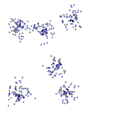
In Figure 1 we show some typical barycenters obtained by our algorithm in this setting. We use smaller datasets for better visibility. In each scenario there are three different point patterns distinguished by the different symbols in black. The (pseudo-)barycenter represented by the blue circles captures the characteristics of each dataset rather well. Some minor irregularities, especially in the third panel may be due to the fact that only a (good) local optimum is computed.
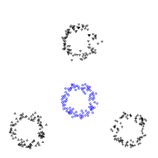
More important than being fast for squared Euclidean distance in is the fact that our algorithm provides a very general umbrella method, that can in principle be used on any underlying space where an appropriate “distance function” between objects is specified as -th power of a metric. All that is required is an algorithm that solves (maybe heuristically) the location problem for individual points in . This allows us e.g. to treat the case of point patterns on a network equipped with the shortest-path metric and . Figure 2 gives an example for crime data in Valencia, Spain, which we study in more detail in Section 6.
The barycenter problem we consider in this paper is closely related to the problem of computing an unbalanced Wasserstein barycenter, see e.g. Chizat et al., (2018). However, rather than minimizing a Fréchet functional on the space of all measures, we minimize on the space of integer valued measures, see Remark 3.2.
The plan of the paper is as follows. In Section 2 we introduce the TT- and RTT-metrics and discuss their relations to spike time, OSPA, and incomplete Wasserstein metrics. Section 3 specifies what we mean by a barycenter (or Fréchet mean) with respect to these metrics and gives an important result that forms the basis for our heuristic algorithm. Two versions of this algorithm, a more direct one and an improved one, which saves computation steps that are unlikely to substantially influence the final result, are discussed in detail in Section 4, along with some practical aspects. Section 5 contains a larger simulation study, which investigates robustness and runtime performances of the two algorithms for the case of Euclidean distance and . Finally, we give two applications to data of crime events on a city map for real data in Section 6. The first one concerns street thefts in Bogotá, Colombia. We treat this again as data in Euclidean space, using . The second one deals with assault cases in the streets of Valencia, Spain. Here we compute barycenters based on the actual shortest-path distance on the street network and use .
2 The transport-transform metric
Denote by the space of finite point patterns (counting measures) on a complete separable metric space , equipped with the usual -algebra generated by the point count maps , for Borel measurable. Elements of are typically denoted by here. As usual we write for the Dirac measure with unit mass at . In the present section we mostly use measure notation such as , or , but in later sections we also use corresponding (multi)set notation such as , or where this is unambiguous.
We use to denote the total number of points in the pattern . For write (including ), and denote by the set of point patterns with exactly points. We first introduce the metrics we use on , which unify and generalize two of the main metrics used previously in the literature.
Definition.
Let and be two parameters, referred to as penalty and order, respectively.
-
(a)
For define the transport-transform (TT) metric by
(2.1) where the minimum is taken over equal numbers of pairwise different indices of and , respectively, i.e.
-
(b)
For define the relative transport-transform (RTT) metric by
(2.2)
We state and prove below that and are indeed metrics.
The following result simplifies proofs of statements about these metrics and is furthermore invaluable for their computation. The idea is to extend the metric space , where , by setting for an auxiliary element and
It is shown in Lemma A.1 that is a metric space again. We may then compute distances in the and metrics by solving an optimal matching problem between point patterns with the same cardinality. For denote by the set of permutations on .
Theorem 2.1.
Let , where w.l.o.g. (otherwise swap and ). Set for and . Then
The proof is found in the appendix.
Remark 2.2 (Computation of TT- and RTT-metrics).
Writing for the maximum cardinality as in Theorem 2.1, this result shows that we can compute both and in worst-time complexity of by using the classic Hungarian method for the assignment problem; see Kuhn, (1955). In practice we use the auction algorithm proposed in Bertsekas, (1988), because it has usually much better runtime in our experience, although the default version has a somewhat worse worst-case performance of .555There is a modified auction algorithm that can improve the worst-case performance to ; for the performance discussion see Bertsekas, (1988), page 109. Actually both orders include a factor in the which measures the numerical precision, assumed to be bounded here.
Proposition 2.3.
The maps and are metrics on .
The proof may be found in the appendix.
Proposition 2.4 (Generalization of previous metrics between point patterns).
-
(a)
If , then for any
(2.3) where the minimum is taken over all and all paths such that , , and from to either a single point is added or deleted at cost or a single point is moved from to at cost .
Thus the TT-metric is the same as the spike time metric (using add and delete penalties and a move penalty ), which was originally introduced on by Victor and Purpura, (1997) and generalized to metric spaces by Diez et al., (2012). - (b)
It can be seen from the proof in the appendix that for the right hand side of (2.3) and for the right hand side of (2.4) will not be metrics in general.
Remark 2.5 (Computation of spike time distances).
The spike time distances in Victor and Purpura, (1997) and Diez et al., (2012) allowed for separate add and delete penalties and , as well as a move penalty (factor in front of ). We set here to obtain a proper metric and divide distances by , which is just a scaling. Thus the parameter is all that remains.
As noted at the end of Section 4 in Diez et al., (2012), having different add and delete penalties may be useful for controlling the total number of points in a barycenter point pattern. Let us point out therefore that Theorem 2.1 is easily adapted to this more general situation by setting , and for all .
In particular this yields a worst-time complexity of for general (maybe asymmetric) spike time distances in general metric spaces, which is a substantial improvement over the complexity of the incremental matching algorithm presented in Diez et al., (2012).
Remark 2.6 (Unbalanced Wasserstein metrics).
The TT- and RTT-metrics can be seen as unbalanced Wasserstein metrics, see e.g. Chizat et al., (2018), Liero et al., (2018) and the references therein. Minimizing over the space of all finite measures on , we obtain the TT-distance as a solution to a particular instance of the unbalanced optimal transport problem in Chizat et al., (2018), Definition 2.11, namely
| (2.5) |
where and denote the marginals of , and is the total variation norm of signed measures; specifically for , where the suprema are taken over all measurable subsets of .
Equation (2.5) can be shown as follows. It is straightforward to see that we may take the infimum on the right hand side only over with marginals and , because any additional mass in may be removed without increasing the total cost of . Writing and with the help of additional points at (if necessary), we obtain by similar arguments as in the proof of Theorem 2.1 that the latter problem is equivalent to the discrete transportation problem
It is a well-known fact from linear programming that this problem always has a solution , ; see e.g. Luenberger and Ye, (2008), Section 6.5. We may therefore conclude from Theorem 2.1 that Equation (2.5) holds and that the infimum on the right hand side is attained for .
In principle, Remark 2.6 allows us to specialize results and algorithms for unbalanced Wasserstein metrics to TT- and RTT-metrics. However, the discrete setting we consider here is sometimes not included in the general theorems or requires a more specialized treatment. Algorithms for computing unbalanced transport plans are typically derived from balanced optimal transport algorithms; a selection can be found in Chizat, (2017). The auction algorithm we use in this paper is derived from the auction algorithm used for balanced assignment problems in a similar way.
3 Barycenters with respect to the TT-metric
For data on quite general metric spaces, barycenters can formalize the idea of a center element representing the data. In the case of we are thus looking for a center point pattern that gives a good first order representation of a set of data point patterns . More formally we may define a barycenter as the (weighted) -th order Fréchet mean with respect to ; see Fréchet, (1948).
Definition.
For let be data point patterns and with be weights. Let furthermore . Then we call any
| (3.1) |
a (weighted) barycenter of order . If no weights are specified we tacitly assume that for , leading to an “unweighted” barycenter.
Remark 3.1.
For barycenters on general metric spaces are simply known as (empirical) Fréchet means. For they are sometimes known as Fréchet medians. This comes from the fact that given , we have
| (3.2) |
(the is unique here), and that given , we have
| (3.3) |
where the right hand side denotes the set of medians .
Remark 3.2.
As seen in Remark 2.6 we may interpret as an unbalanced Wasserstein metric. There has been a great deal of research on Wasserstein barycenters (in the Fréchet mean sense as above, see e.g. Agueh and Carlier, (2011) or Cuturi and Doucet, (2014)), which more recently also extends to unbalanced Wasserstein metrics, see e.g. Chizat et al., (2018) or Schmitz et al., (2018). In addition to the fact that much of the corresponding theory is not well adapted to the case of discrete input measures, with the notable exception of Anderes et al., (2016), we point out that a fundamental difference of (3.1) lies in the fact that we minimize over the space of integer-valued rather than general measures.
In what follows we always set and choose this number mostly . We refer to the resulting barycenters simply as - and -barycenter or as point pattern median and point pattern mean, respectively. Point pattern medians have been introduced under the name of prototypes in Schoenberg and Tranbarger, (2008) on and studied in higher dimensions in Diez et al., (2012) and Mateu et al., (2015). However, in these papers the applicability was limited to rather small datasets due to the large computation cost of mentioned in Remark 2.5.
Using the construction from Theorem 2.1, we may reformulate the barycenter problem as a multidimensional assignment problem, generalizing Lemma 16 in Koliander et al., (2018). Note that for the TT-metric we can add an arbitrary number of points at to both point patterns without changing the minimum in Theorem 2.1.
Proposition 3.3.
For point patterns , , let and . Set for and for any .
Then for any jointly minimizing
| (3.4) |
the point pattern with , where is a -th order barycenter with respect to the TT-metric.
The above define disjoint “clusters” , where each contains exactly one (maybe virtual) point of each point pattern. The minimization of (3.4) may thus be interpreted as a multidimensional assignment problem with cluster cost
| (3.5) |
Proof.
Let us first give an upper bound on the cardinality of the barycenter. A single barycenter point can be matched with up to points (one from each point pattern). If said point is matched with only points or fewer, it cannot be worse to delete it. The contribution for this point in the objective function is at least , while deleting it adds at most to the objective function.
So every barycenter point should be matched with at least points. The total number of points is . Therefore the number of barycenter points is bounded above by .
It is thus sufficient to fill up all the point patterns to points and work also with an ansatz of points for . Theorem 2.1 yields
| (3.6) |
and that any minimizer on the left hand side is obtained from jointly minimizing in and on the right hand side. ∎
4 Alternating clustering algorithms
Based on Proposition 3.3 we propose an algorithm that alternates between minimizing
| (4.1) |
in and in until convergence. Such an algorithm terminates in a local minimum of (4.1) after a finite number of steps, because (4.1) can never increase and the minimization in the permutations is over a finite space.
Since this underlying idea is similar to the popular -means clustering algorithm, we named the main function in the pseudocode and in the actual implementation kMeansBary (note, however, that plays the role of in our notation). A similar algorithm in the quite different setting of trimmed Wasserstein-2 barycenters for finitely supported probability measures is proposed in del Barrio et al., (2019).
In what follows we present pseudocode along with the underlying ideas and explanations for two versions of the kMeansBary-algorithm that we dub original and improved. Here “improved” refers to the fact that we cut down on certain computation steps in order to save runtime. We will see in Section 5 that this comes essentially without any performance loss.
User-friendly implementations of both algorithms will be made publicly available in an R-package.
4.1 Our original kMeansBary algorithm
The pseudocode for the basic alternating strategy described above is given in Algorithm 1. We have introduced a stopping parameter to allow termination before the local optimum is reached. Since we are not interested in the actual clustering, but only in the position of the centers , it seems very unlikely (though possible) that the solution changes substantially once the cost decrease has become very small. What is more, such a change might be spurious due to rounding errors in the data or when we use an approximation method for optimizing in the centers. Note also that we can always set to the smallest representable positive floating-point number to ensure convergence to the local optimum.
The minimization with respect to is performed by optimPerm. This function computes an optimal matching between the current center and each data point pattern in pplist, using an alternating version of the auction algorithm with -scaling; see Remark 2.2 and Bertsekas, (1988) for more details. We output the cost of the current matching and an matrix perm, whose -th column specifies the order in which the points of the -th data pattern are matched to . For greater efficiency we save auxiliary information (price and profit vectors) and use it for initializing the auction algorithm when calling it again with the same data point pattern.
For practical purposes we have split up the minimization with respect to into a function optimBary that optimizes the positions within and functions optimDelete and optimAdd that optimize which of the to move from to and from to , respectively. We discuss details of these functions below.
In addition to the outputs of the various functions shown in Algorithm 1, we also keep information on the quality of each match of points up to date. We call the match of a with a data point
Note that a miserable match is worst possible in the sense that for center cannot increase if is replaced by any other .
optimBary
The purpose of this function is to find for each (i.e. not currently at ) a location in that minimizes for its current cluster . This amounts to a more traditional location problem in , except that it is typically made (much) more difficult by the fact that we have to truncate distances at .
Note that any cluster points at can be ignored because they always contribute the same amount to the cluster cost, no matter where the center lies. The same is true for individual points that have a much larger distance than from the bulk of the points. However, there are countless scenarios with (groups of) points being around distance apart from one another for which the optimization of the cluster cost becomes a difficult optimization problem (piecewise smooth on a space that is fragmented in complicated ways).
As a simple heuristic that works well in cases where we do not have to cut too many distances (i.e. is not too small), we suggest to ignore all points that are at the maximal -distance from the current when computing the new . Note that in this way the cluster cost can never increase.
Algorithm 2 gives corresponding pseudocode. The function optimClusterCenter handles the location problem for the untruncated metric on . If for example equipped with the Euclidean metric and , Equation (3.2) implies that optimClusterCenter simply has to take the (coordinatewise) average of all happy points. The case can be tackled with higher computational effort by approximation via the popular Weiszfeld algorithm; see Weiszfeld, (1937).
As a further instance, which we will take up in Section 6, we consider the situation where is a simple graph equipped with the shortest-path distance and . It can be shown that in this case the location problem in is solved by an element of , i.e. either a vertex of the graph or any data point, see Hakimi, (1964). We therefore proceed by first computing the distance matrix between all these points, which is then used for the entire algorithm. Such shortest-path distance computations in sparse graphs with thousands of points can be performed in (at most) a few seconds by various algorithms, see Chapter 25 in Cormen et al., (2009) and the concrete timing in Subsection 6.2. It is now easy to implement the function optimClusterCenter. For a given set of happy points of a cluster , pick the corresponding columns in the distance matrix, add them up and determine the minimal entry of the resulting vector. If there are several such entries, which due to choosing can happen quite frequently, we pick one among them uniformly at random. The index of the obtained entry identifies the center point .
Note that precomputing the distance matrix between all points in has the additional advantage that no distances have to be computed in the optimPerm step.
optimDelete
This function deletes (i.e. moves to ) any for which this operation decreases .
We denote by , and the numbers of data points in that are happy, miserable and at , respectively. Write furthermore for the total cost of matching the happy points to . If stays in the cluster incurs an overall total cost of
as opposed to
if we delete . Subtracting from both expressions this leads to the deletion condition
Since , a sufficient condition for deletion is . We use this as a quick pre-test, which allows us to avoid computing sometimes. The full deletion procedure is presented in Algorithm 3.
optimAdd
This function adds (i.e. moves to ) any for which it finds a way to do so that decreases . Pseudocode is given in Algorithm 4.
As a compromise between computational simplicity and finding a good location in , we first sample a proposal location uniformly from all miserable data points (i.e. points from any cluster that are currently in a miserable match with their center). Before we consider moving to , we rebuild the cluster in such a way that this move has a better chance of being accepted.
The corresponding procedure is performed by the optimizeCluster-function in the pseudocode: For each data pattern pick the miserable point that is closest to (if it has any) and exchange it with the corresponding point that is currently in . Since the point coming from the other cluster was miserable before, the cost of that cluster cannot increase by this exchange. The cost of the cluster can increase only if it loses a point located at in the exchange. In this case the cost increases by , which is compensated by the fact that the cost of the other cluster must decrease, either from to if its center is in , or from to if its center is at . Thus the total cost remains the same, but has an additional point in now, which makes the successful addition of to more likely.
To further decrease the prospective cluster cost after addition, we update the proposal by recentering it in its new cluster using the appropriate optimClusterCenter-function introduced in optimBary (applied to the set of points of the new cluster that are in a happy match with ).
Finally, check whether the cost of the new cluster based on the updated is smaller than the same cost based on , which is times the number of non- points in the new cluster. Set to if this is the case.
4.2 An improved kMeansBary algorithm
For obtaining an algorithm with a reduced computational cost, we cut down on steps that are costly, but are not expected to influence the resulting local optimum in a decisive way. Since for now we treat the location problem at the cluster level (performed by optimBary) as very general, allowing a wide range of metric spaces , we focus here on saving computations in the functions optimPerm, optimDelete, and optimAdd.
We have realized that by far the most additions and deletions of points take place in the first two iterations of the original algorithm (see also Figure 3 below). Especially checking for addition of points is costly and after the first few iterations very rarely successful. Therefore we limit such checking henceforward to the first iteration steps. Some further heuristics could be applied in optimAdd, but the gain in computation time is not so large and they can significantly change the outcome, which is why we decided against implementing them.
In optimPerm we cannot avoid doing matchings. However, the auction algorithm we use allows to solve a relaxation of the problem by stopping the -scaling method early. In general, the auction algorithm with -scaling based on a decreasing sequence returns successively improved solutions that are guaranteed to lie within of the optimal total cost after the -th step, see Bertsekas, (1988, Proposition 1). By representing rescaled distances as integers in , an optimal matching is obtained in the -th step if . Our improved algorithm is based on the same -vector as the original algorithm, which has components , , where is chosen in such a way that . As a first improvement, we use the subsequence , where and are prespecified vectors of indices . A simple choice for and that tends to decrease the runtime noticeably is and . Pseudocode for this is presented in Algorithm 5.
In practice we settled for a somewhat more sophisticated improvement. We choose and , and we use the sequence , where for , and then is increased by each time the algorithm would otherwise converge or if the cost increases (which can only happen as long as the matchings are not optimal).
This strategy was chosen after analyzing the calculations of the algorithm with respect to the time each calculation takes. In the first two to three iterations there are a lot of changes in the positions of the barycenter points. Especially in the first iteration many points are deleted and added, which completely changes the assignments. Therefore we have to begin the assignment calculation with and to get more sensible results we get more precise with each of the first three iterations. After three iterations there are usually no big changes to the barycenter anymore, so we can reuse the assignment from the iteration before as a sensible starting solution and can omit and in return. Leaving out the first entries of too soon increases the runtime. Every time the algorithm converges, but has no guaranteed optimal assignment (i.e. ), is increased by , meaning that the next two entries of are used too, until the end of is reached. Then we can safely leave out the first three entries of without increasing the runtime, because at this point the assignments from one iteration to the next only change very little.
4.3 Practical aspects
As it turns out the upper bound on the cardinality of the barycenter from Proposition 3.3 is often far too large in practice. For efficiency reasons we typically run the algorithm with a number that is much smaller than . We generate a starting point pattern center by picking points uniformly at random from the underlying observation window. In a first step all point patterns are filled to points by adding points at . Then Algorithm 1 or 5 is run.
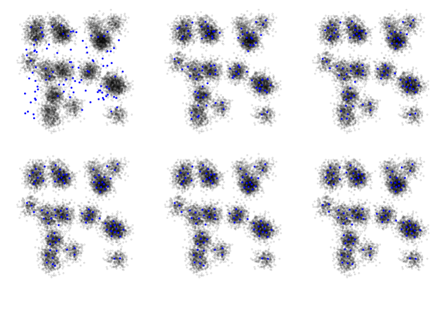
Figure 3 shows a typical run of Algorithm 1 in the case of an i.i.d. sample of point patterns in generated from a similar distribution as studied in Section 5. We use Euclidean distance and . The current barycenter is marked by blue points. Typically the random starting point pattern is not a good approximation to the resulting barycenter. Therefore many points are deleted in the first iteration. Many other ones are added at or moved to more cost efficient spots. Regardless of the starting pattern the algorithm typically attains a reasonably looking configuration after a single iteration. After that hardly any points are added or deleted any more. The algorithm mostly moves a few individual barycenter points around each time.
5 Simulation study
In this section we present a simulation study for evaluating the algorithms described in Section 4 for point patterns in using squared Euclidean cost. Unfortunately it is not feasible for larger data examples to compute the actual barycenter as a ground truth. Even when treating the point patterns as empirical measures and solving the simpler and much better studied problem of finding a barycenter in the space of probability measures (with respect to the Wasserstein metric ), the computation times for problems close to our smallest examples below range from minutes to hours; see Anderes et al., (2016) and Borgwardt and Patterson, (2018). As a replacement of comparing with the actual barycenter, we assess the range of the final objective function values. In addition we evaluate the time performance of the default algorithm, and compare both objective function values and timings to the improved algorithm.
As problem instances we created sets of point patterns in having mean cardinality of in each pattern. The cardinalities , , of the individual point patterns were determined by one of the following methods:
-
(i)
by setting (deterministic cardinality)
-
(ii)
by sampling from a binomial distribution with mean and variance
(low-variance cardinality) -
(iii)
by sampling from a Poisson distribution with parameter
(high-variance cardinality)
The points were distributed according to a balanced mixture of rotationally symmetric normal densities centered at fixed locations in and having standard deviation . Figure 4 gives examples under the three center scenarios for , deterministic cardinality and .


We chose five pairs and , which in combination with varying in , in and the three cardinality distributions yield a total of scenarios. We created instances for each scenario.
Our algorithms from Section 4 were run from ten starting solutions whose cardinalities matched the mean number of data points and whose points were sampled uniformly at random from . In a pilot experiment this tended to give somewhat better local minima than starting from a random sample of all data points combined. The starting point patterns were independently chosen for each instance, but the same for both algorithms.
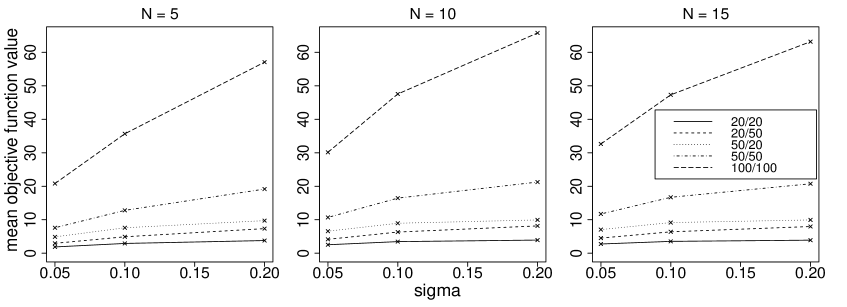
We first consider the original algorithm presented in Section 4. Table 1 gives the maximum relative deviation from the minimum of the resulting objective function values among the ten starting solutions, i.e. . We can see that the maximal objective function value among the ten runs rarely exceeds the minimum value by more than 5%. This percentage is rather higher for the deterministic and low-variance cardinalities and when clusters in the (unmarked) superposition of the point patterns are well separated (small and ). This may well be explicable by the fact that typically many pairs can be matched over short distances in these situations such that wrong clustering decisions come typically at a higher relative cost. Figure 5 supports this by showing that the total objective function values within each problem size are lower for well separated clusters.
A further smaller experiment following up on the scenarios that exhibited the poorest performance for ten starting patterns showed that the margin of 5% increases to 8% when basing the maximum relative deviation from the minimum on 100 starting patterns.
For the improved algorithm from Subsection 4.2 we compute the maximum relative deviation of its objective function values from the minimum of the corresponding values of the original algorithm, i.e. , where is the maximum of the objective function values of the improved algorithm. As seen in Table 2 the performance is no worse than for the original algorithm in spite of the reduced amount of computations performed.
| N | 20/20 | 20/50 | 50/20 | 50/50 | 100/100 | |
| 0.05 | 0.05 (0.03, 0.07) | 0.04 (0.02, 0.06) | 0.04 (0.03, 0.06) | 0.04 (0.02, 0.05) | 0.03 (0.02, 0.05) | |
| 5 | 0.1 | 0.04 (0.02, 0.06) | 0.03 (0.02, 0.05) | 0.03 (0.02, 0.04) | 0.03 (0.02, 0.04) | 0.03 (0.02, 0.05) |
| 0.2 | 0.02 (0.01, 0.03) | 0.02 (0.01, 0.03) | 0.01 (0.01, 0.02) | 0.02 (0.01, 0.02) | 0.01 (0.01, 0.02) | |
| 0.05 | 0.04 (0.02, 0.06) | 0.04 (0.02, 0.06) | 0.03 (0.02, 0.05) | 0.03 (0.02, 0.05) | 0.03 (0.02, 0.05) | |
| 10 | 0.1 | 0.02 (0.02, 0.04) | 0.03 (0.02, 0.04) | 0.02 (0.01, 0.03) | 0.02 (0.01, 0.03) | 0.02 (0.01, 0.03) |
| 0.2 | 0.01 (0.00, 0.02) | 0.02 (0.01, 0.03) | 0.00 (0.00, 0.01) | 0.01 (0.01, 0.02) | 0.01 (0.01, 0.01) | |
| 0.05 | 0.03 (0.02, 0.05) | 0.03 (0.02, 0.05) | 0.03 (0.01, 0.04) | 0.03 (0.02, 0.04) | 0.03 (0.02, 0.04) | |
| 15 | 0.1 | 0.02 (0.01, 0.04) | 0.03 (0.02, 0.04) | 0.02 (0.01, 0.02) | 0.02 (0.01, 0.03) | 0.02 (0.01, 0.02) |
| 0.2 | 0.02 (0.01, 0.03) | 0.02 (0.01, 0.03) | 0.01 (0.00, 0.01) | 0.01 (0.01, 0.02) | 0.01 (0.01, 0.01) | |
| 0.05 | 0.05 (0.03, 0.07) | 0.04 (0.02, 0.05) | 0.04 (0.02, 0.06) | 0.04 (0.02, 0.05) | 0.03 (0.02, 0.05) | |
| 5 | 0.1 | 0.04 (0.02, 0.05) | 0.03 (0.02, 0.05) | 0.03 (0.01, 0.04) | 0.03 (0.02, 0.04) | 0.03 (0.02, 0.05) |
| 0.2 | 0.02 (0.01, 0.03) | 0.02 (0.01, 0.04) | 0.01 (0.01, 0.02) | 0.02 (0.01, 0.02) | 0.01 (0.01, 0.02) | |
| 0.05 | 0.03 (0.02, 0.06) | 0.04 (0.02, 0.06) | 0.03 (0.02, 0.04) | 0.03 (0.02, 0.05) | 0.04 (0.02, 0.05) | |
| 10 | 0.1 | 0.02 (0.01, 0.04) | 0.03 (0.02, 0.04) | 0.02 (0.01, 0.03) | 0.02 (0.01, 0.03) | 0.02 (0.01, 0.03) |
| 0.2 | 0.01 (0.01, 0.02) | 0.02 (0.01, 0.03) | 0.01 (0.00, 0.01) | 0.01 (0.01, 0.02) | 0.01 (0.01, 0.01) | |
| 0.05 | 0.03 (0.02, 0.05) | 0.03 (0.02, 0.05) | 0.02 (0.01, 0.04) | 0.03 (0.02, 0.04) | 0.03 (0.01, 0.04) | |
| 15 | 0.1 | 0.02 (0.01, 0.04) | 0.03 (0.02, 0.04) | 0.01 (0.01, 0.02) | 0.02 (0.01, 0.03) | 0.02 (0.01, 0.02) |
| 0.2 | 0.01 (0.01, 0.02) | 0.02 (0.01, 0.03) | 0.01 (0.00, 0.01) | 0.02 (0.01, 0.02) | 0.01 (0.01, 0.01) | |
| 0.05 | 0.03 (0.02, 0.05) | 0.02 (0.01, 0.04) | 0.03 (0.01, 0.04) | 0.02 (0.01, 0.03) | 0.01 (0.01, 0.02) | |
| 5 | 0.1 | 0.03 (0.02, 0.05) | 0.03 (0.02, 0.04) | 0.02 (0.01, 0.04) | 0.02 (0.01, 0.03) | 0.02 (0.01, 0.03) |
| 0.2 | 0.02 (0.01, 0.03) | 0.02 (0.01, 0.03) | 0.01 (0.01, 0.01) | 0.02 (0.01, 0.02) | 0.01 (0.01, 0.02) | |
| 0.05 | 0.03 (0.02, 0.04) | 0.03 (0.01, 0.04) | 0.02 (0.01, 0.04) | 0.02 (0.01, 0.04) | 0.02 (0.01, 0.03) | |
| 10 | 0.1 | 0.02 (0.01, 0.04) | 0.02 (0.01, 0.03) | 0.01 (0.01, 0.02) | 0.02 (0.01, 0.03) | 0.01 (0.01, 0.02) |
| 0.2 | 0.01 (0.00, 0.02) | 0.02 (0.01, 0.03) | 0.00 (0.00, 0.01) | 0.01 (0.01, 0.02) | 0.01 (0.01, 0.01) | |
| 0.05 | 0.03 (0.01, 0.04) | 0.03 (0.02, 0.04) | 0.02 (0.01, 0.04) | 0.02 (0.01, 0.03) | 0.01 (0.01, 0.02) | |
| 15 | 0.1 | 0.02 (0.01, 0.03) | 0.03 (0.01, 0.04) | 0.01 (0.01, 0.02) | 0.02 (0.01, 0.03) | 0.01 (0.01, 0.02) |
| 0.2 | 0.01 (0.00, 0.02) | 0.02 (0.01, 0.03) | 0.00 (0.00, 0.01) | 0.01 (0.01, 0.02) | 0.01 (0.01, 0.02) |
| N | 20/20 | 20/50 | 50/20 | 50/50 | 100/100 | |
| 0.05 | 0.04 (0.02, 0.06) | 0.04 (0.02, 0.06) | 0.04 (0.02, 0.06) | 0.04 (0.02, 0.06) | 0.03 (0.02, 0.05) | |
| 5 | 0.1 | 0.04 (0.02, 0.06) | 0.03 (0.02, 0.05) | 0.03 (0.02, 0.04) | 0.03 (0.02, 0.04) | 0.03 (0.02, 0.05) |
| 0.2 | 0.02 (0.01, 0.03) | 0.02 (0.02, 0.03) | 0.01 (0.00, 0.02) | 0.02 (0.01, 0.02) | 0.01 (0.01, 0.02) | |
| 0.05 | 0.04 (0.02, 0.06) | 0.04 (0.02, 0.05) | 0.03 (0.02, 0.05) | 0.04 (0.02, 0.05) | 0.03 (0.02, 0.05) | |
| 10 | 0.1 | 0.02 (0.01, 0.03) | 0.03 (0.02, 0.04) | 0.02 (0.01, 0.02) | 0.02 (0.01, 0.03) | 0.02 (0.01, 0.03) |
| 0.2 | 0.01 (0.00, 0.02) | 0.02 (0.01, 0.03) | 0.00 (0.00, 0.01) | 0.02 (0.01, 0.02) | 0.01 (0.01, 0.01) | |
| 0.05 | 0.03 (0.02, 0.05) | 0.03 (0.02, 0.05) | 0.03 (0.01, 0.04) | 0.03 (0.02, 0.04) | 0.03 (0.02, 0.04) | |
| 15 | 0.1 | 0.02 (0.01, 0.04) | 0.03 (0.02, 0.04) | 0.02 (0.01, 0.02) | 0.02 (0.01, 0.03) | 0.02 (0.01, 0.02) |
| 0.2 | 0.01 (0.00, 0.02) | 0.02 (0.01, 0.03) | 0.00 (0.00, 0.01) | 0.02 (0.01, 0.02) | 0.01 (0.01, 0.01) | |
| 0.05 | 0.04 (0.02, 0.07) | 0.04 (0.02, 0.05) | 0.04 (0.02, 0.06) | 0.03 (0.02, 0.05) | 0.03 (0.02, 0.05) | |
| 5 | 0.1 | 0.03 (0.02, 0.05) | 0.03 (0.02, 0.05) | 0.03 (0.01, 0.04) | 0.03 (0.02, 0.04) | 0.03 (0.02, 0.04) |
| 0.2 | 0.02 (0.01, 0.03) | 0.03 (0.01, 0.04) | 0.01 (0.00, 0.02) | 0.02 (0.01, 0.03) | 0.01 (0.01, 0.02) | |
| 0.05 | 0.03 (0.02, 0.05) | 0.03 (0.02, 0.06) | 0.03 (0.01, 0.04) | 0.03 (0.02, 0.05) | 0.04 (0.02, 0.05) | |
| 10 | 0.1 | 0.02 (0.01, 0.04) | 0.03 (0.01, 0.04) | 0.02 (0.01, 0.02) | 0.02 (0.01, 0.03) | 0.02 (0.01, 0.03) |
| 0.2 | 0.01 (0.00, 0.02) | 0.02 (0.01, 0.03) | 0.00 (0.00, 0.01) | 0.01 (0.01, 0.02) | 0.01 (0.01, 0.01) | |
| 0.05 | 0.03 (0.02, 0.05) | 0.03 (0.02, 0.04) | 0.02 (0.01, 0.04) | 0.03 (0.02, 0.04) | 0.02 (0.01, 0.04) | |
| 15 | 0.1 | 0.02 (0.01, 0.03) | 0.03 (0.02, 0.04) | 0.01 (0.01, 0.02) | 0.02 (0.01, 0.03) | 0.01 (0.01, 0.02) |
| 0.2 | 0.01 (0.00, 0.02) | 0.02 (0.02, 0.03) | 0.00 (0.00, 0.01) | 0.02 (0.01, 0.02) | 0.01 (0.00, 0.01) | |
| 0.05 | 0.03 (0.02, 0.05) | 0.02 (0.01, 0.03) | 0.03 (0.01, 0.04) | 0.02 (0.01, 0.03) | 0.01 (0.00, 0.02) | |
| 5 | 0.1 | 0.03 (0.02, 0.04) | 0.03 (0.01, 0.04) | 0.02 (0.01, 0.04) | 0.02 (0.01, 0.03) | 0.02 (0.01, 0.03) |
| 0.2 | 0.02 (0.01, 0.03) | 0.02 (0.01, 0.03) | 0.01 (0.00, 0.01) | 0.02 (0.01, 0.02) | 0.01 (0.01, 0.02) | |
| 0.05 | 0.03 (0.01, 0.04) | 0.03 (0.01, 0.04) | 0.02 (0.01, 0.04) | 0.02 (0.01, 0.03) | 0.02 (0.01, 0.03) | |
| 10 | 0.1 | 0.02 (0.01, 0.03) | 0.02 (0.02, 0.04) | 0.01 (0.01, 0.02) | 0.02 (0.01, 0.03) | 0.01 (0.01, 0.02) |
| 0.2 | 0.01 (0.00, 0.02) | 0.02 (0.01, 0.03) | 0.00 (0.00, 0.01) | 0.01 (0.01, 0.02) | 0.01 (0.01, 0.01) | |
| 0.05 | 0.02 (0.01, 0.04) | 0.02 (0.02, 0.04) | 0.02 (0.01, 0.04) | 0.02 (0.01, 0.03) | 0.01 (0.01, 0.02) | |
| 15 | 0.1 | 0.02 (0.01, 0.03) | 0.02 (0.01, 0.04) | 0.01 (0.01, 0.02) | 0.02 (0.01, 0.03) | 0.01 (0.01, 0.02) |
| 0.2 | 0.01 (0.00, 0.01) | 0.02 (0.01, 0.03) | 0.00 (0.00, 0.01) | 0.01 (0.01, 0.02) | 0.01 (0.01, 0.02) |
We finally turn to the computation times. We present the total runtimes in seconds for the ten runs with different starting patterns. This corresponds to the realistic situation of selecting as (pseudo-)barycenter the solution with the smallest local minimum in ten runs. It also provides some more stability for the means and quantiles given in Tables 3 and 4.
Table 3 gives the runtimes for the original algorithm. We see that individual runs of as large scenarios as 100 patterns with 100 points on average only take a few seconds.
From Table 4 we see that the runtimes for the improved algorithm are even considerably lower, and for some of the larger problems they have less than half of the original runtimes (at virtually no loss with regard to the objective function value as we have seen before). It is to be expected that this ratio becomes even smaller if the problem size is further increased.
| N | 20/20 | 20/50 | 50/20 | 50/50 | 100/100 | |
| 0.05 | 0.48 (0.47, 0.50) | 0.89 (0.85, 0.93) | 1.02 (0.99, 1.05) | 2.37 (2.24, 2.52) | 20.79 (19.42, 22.32) | |
| 5 | 0.1 | 0.52 (0.51, 0.54) | 1.05 (0.99, 1.10) | 1.14 (1.10, 1.19) | 3.13 (2.92, 3.36) | 30.26 (27.51, 32.92) |
| 0.2 | 0.51 (0.49, 0.53) | 1.14 (1.07, 1.23) | 1.05 (0.99, 1.12) | 3.55 (3.26, 3.96) | 37.95 (34.70, 42.22) | |
| 0.05 | 0.49 (0.48, 0.51) | 0.93 (0.89, 0.97) | 1.05 (1.01, 1.08) | 2.49 (2.37, 2.64) | 22.15 (20.33, 24.63) | |
| 10 | 0.1 | 0.52 (0.51, 0.54) | 1.08 (1.03, 1.15) | 1.14 (1.09, 1.20) | 3.18 (2.96, 3.47) | 33.83 (30.03, 37.89) |
| 0.2 | 0.48 (0.45, 0.50) | 1.16 (1.10, 1.24) | 0.91 (0.85, 0.97) | 3.56 (3.27, 3.91) | 40.30 (36.14, 44.69) | |
| 0.05 | 0.50 (0.49, 0.51) | 0.95 (0.91, 1.00) | 1.06 (1.03, 1.09) | 2.60 (2.44, 2.80) | 24.25 (22.51, 25.93) | |
| 15 | 0.1 | 0.52 (0.50, 0.53) | 1.08 (1.02, 1.15) | 1.13 (1.08, 1.17) | 3.20 (2.93, 3.53) | 32.70 (29.62, 35.91) |
| 0.2 | 0.49 (0.47, 0.51) | 1.14 (1.08, 1.22) | 0.91 (0.85, 0.99) | 3.51 (3.12, 3.85) | 37.77 (33.86, 42.21) | |
| 0.05 | 0.51 (0.49, 0.53) | 0.92 (0.89, 0.96) | 1.05 (1.02, 1.08) | 2.51 (2.38, 2.67) | 21.43 (19.89, 23.47) | |
| 5 | 0.1 | 0.53 (0.52, 0.54) | 1.08 (1.02, 1.13) | 1.17 (1.12, 1.22) | 3.20 (3.00, 3.44) | 30.93 (28.03, 33.42) |
| 0.2 | 0.54 (0.51, 0.57) | 1.18 (1.10, 1.25) | 1.08 (1.00, 1.15) | 3.71 (3.34, 4.06) | 38.97 (34.69, 42.74) | |
| 0.05 | 0.51 (0.49, 0.52) | 0.96 (0.91, 1.00) | 1.07 (1.04, 1.11) | 2.57 (2.42, 2.73) | 22.70 (20.97, 24.87) | |
| 10 | 0.1 | 0.54 (0.52, 0.56) | 1.12 (1.06, 1.20) | 1.17 (1.12, 1.23) | 3.36 (3.07, 3.68) | 34.18 (30.47, 37.91) |
| 0.2 | 0.49 (0.46, 0.51) | 1.19 (1.12, 1.27) | 0.93 (0.87, 1.00) | 3.72 (3.35, 4.11) | 41.21 (35.90, 46.22) | |
| 0.05 | 0.51 (0.50, 0.53) | 0.98 (0.94, 1.03) | 1.09 (1.06, 1.13) | 2.70 (2.51, 2.93) | 25.07 (22.73, 27.86) | |
| 15 | 0.1 | 0.53 (0.52, 0.55) | 1.11 (1.05, 1.19) | 1.17 (1.12, 1.22) | 3.34 (3.11, 3.62) | 33.94 (30.91, 37.06) |
| 0.2 | 0.50 (0.46, 0.52) | 1.19 (1.13, 1.26) | 0.93 (0.87, 1.03) | 3.66 (3.35, 3.95) | 38.60 (35.05, 42.61) | |
| 0.05 | 0.58 (0.53, 0.64) | 1.27 (1.11, 1.53) | 1.37 (1.24, 1.55) | 4.12 (3.38, 4.97) | 39.66 (33.33, 46.96) | |
| 5 | 0.1 | 0.62 (0.57, 0.69) | 1.46 (1.26, 1.74) | 1.57 (1.36, 1.83) | 5.04 (4.05, 6.12) | 55.56 (45.67, 65.94) |
| 0.2 | 0.59 (0.53, 0.67) | 1.58 (1.37, 1.88) | 1.30 (1.11, 1.47) | 5.62 (4.64, 6.86) | 65.86 (54.51, 77.49) | |
| 0.05 | 0.59 (0.54, 0.65) | 1.27 (1.09, 1.51) | 1.36 (1.24, 1.55) | 4.10 (3.38, 4.99) | 41.13 (35.65, 47.79) | |
| 10 | 0.1 | 0.60 (0.55, 0.67) | 1.48 (1.29, 1.79) | 1.48 (1.29, 1.68) | 5.14 (4.34, 6.14) | 60.16 (50.16, 70.58) |
| 0.2 | 0.54 (0.49, 0.61) | 1.60 (1.37, 1.87) | 1.06 (0.94, 1.23) | 5.66 (4.62, 6.80) | 69.19 (58.12, 83.04) | |
| 0.05 | 0.59 (0.55, 0.65) | 1.32 (1.16, 1.56) | 1.41 (1.26, 1.64) | 4.31 (3.59, 5.22) | 45.37 (38.88, 51.93) | |
| 15 | 0.1 | 0.61 (0.55, 0.70) | 1.46 (1.24, 1.69) | 1.47 (1.31, 1.66) | 5.27 (4.42, 6.41) | 60.57 (50.30, 70.68) |
| 0.2 | 0.55 (0.49, 0.61) | 1.55 (1.37, 1.81) | 1.06 (0.94, 1.23) | 5.73 (4.72, 7.23) | 66.25 (56.73, 79.16) |
| N | 20/20 | 20/50 | 50/20 | 50/50 | 100/100 | |
| 0.05 | 0.48 (0.47, 0.48) | 0.83 (0.81, 0.85) | 0.97 (0.96, 0.99) | 2.05 (1.99, 2.12) | 13.68 (13.02, 14.57) | |
| 5 | 0.1 | 0.50 (0.49, 0.50) | 0.92 (0.89, 0.96) | 1.03 (1.01, 1.05) | 2.42 (2.29, 2.60) | 16.51 (15.38, 17.85) |
| 0.2 | 0.50 (0.49, 0.50) | 0.93 (0.89, 0.98) | 1.00 (0.98, 1.02) | 2.47 (2.33, 2.65) | 18.25 (16.87, 20.57) | |
| 0.05 | 0.48 (0.48, 0.49) | 0.84 (0.82, 0.87) | 0.98 (0.97, 1.00) | 2.06 (1.97, 2.14) | 13.22 (12.43, 14.01) | |
| 10 | 0.1 | 0.50 (0.49, 0.51) | 0.92 (0.88, 0.96) | 1.03 (1.01, 1.05) | 2.38 (2.23, 2.53) | 16.94 (15.61, 19.17) |
| 0.2 | 0.49 (0.48, 0.50) | 0.94 (0.91, 0.98) | 0.96 (0.92, 0.98) | 2.46 (2.34, 2.63) | 18.84 (17.24, 20.60) | |
| 0.05 | 0.49 (0.48, 0.49) | 0.85 (0.82, 0.88) | 0.98 (0.97, 1.00) | 2.08 (1.99, 2.20) | 13.24 (12.47, 14.26) | |
| 15 | 0.1 | 0.50 (0.49, 0.51) | 0.90 (0.87, 0.95) | 1.02 (1.00, 1.04) | 2.36 (2.25, 2.52) | 16.22 (14.72, 18.07) |
| 0.2 | 0.50 (0.49, 0.50) | 0.92 (0.89, 0.95) | 0.96 (0.92, 0.99) | 2.42 (2.27, 2.57) | 17.62 (16.08, 19.33) | |
| 0.05 | 0.50 (0.49, 0.52) | 0.86 (0.84, 0.88) | 1.00 (0.98, 1.02) | 2.13 (2.06, 2.21) | 14.07 (13.58, 14.80) | |
| 5 | 0.1 | 0.51 (0.50, 0.51) | 0.94 (0.91, 0.98) | 1.05 (1.03, 1.08) | 2.46 (2.35, 2.60) | 16.99 (15.77, 18.57) |
| 0.2 | 0.52 (0.51, 0.54) | 0.95 (0.92, 0.99) | 1.02 (1.00, 1.04) | 2.53 (2.38, 2.73) | 18.72 (17.26, 20.73) | |
| 0.05 | 0.49 (0.49, 0.50) | 0.87 (0.84, 0.90) | 1.01 (0.99, 1.03) | 2.12 (2.04, 2.24) | 13.28 (12.62, 14.02) | |
| 10 | 0.1 | 0.51 (0.50, 0.52) | 0.94 (0.90, 0.98) | 1.05 (1.03, 1.08) | 2.41 (2.30, 2.55) | 17.05 (15.60, 18.85) |
| 0.2 | 0.50 (0.49, 0.51) | 0.95 (0.93, 0.99) | 0.98 (0.95, 1.01) | 2.50 (2.37, 2.67) | 19.47 (17.74, 21.83) | |
| 0.05 | 0.49 (0.49, 0.50) | 0.87 (0.84, 0.90) | 1.01 (0.99, 1.03) | 2.15 (2.06, 2.25) | 13.62 (12.79, 14.66) | |
| 15 | 0.1 | 0.51 (0.50, 0.52) | 0.92 (0.88, 0.96) | 1.04 (1.02, 1.06) | 2.39 (2.26, 2.58) | 16.69 (15.14, 18.99) |
| 0.2 | 0.50 (0.50, 0.51) | 0.95 (0.91, 0.98) | 0.98 (0.95, 1.01) | 2.48 (2.35, 2.68) | 18.16 (16.50, 20.29) | |
| 0.05 | 0.56 (0.52, 0.61) | 1.14 (1.00, 1.33) | 1.24 (1.14, 1.36) | 3.21 (2.82, 3.73) | 22.47 (19.86, 25.53) | |
| 5 | 0.1 | 0.58 (0.54, 0.64) | 1.22 (1.07, 1.40) | 1.31 (1.18, 1.45) | 3.65 (3.10, 4.32) | 26.79 (23.16, 31.02) |
| 0.2 | 0.58 (0.54, 0.63) | 1.23 (1.09, 1.43) | 1.21 (1.12, 1.30) | 3.64 (3.25, 4.18) | 29.41 (25.54, 34.47) | |
| 0.05 | 0.56 (0.53, 0.60) | 1.11 (0.97, 1.28) | 1.23 (1.13, 1.37) | 3.10 (2.71, 3.54) | 21.82 (19.13, 24.59) | |
| 10 | 0.1 | 0.57 (0.53, 0.63) | 1.19 (1.05, 1.38) | 1.27 (1.15, 1.41) | 3.51 (3.02, 4.17) | 27.49 (23.81, 32.18) |
| 0.2 | 0.56 (0.52, 0.61) | 1.22 (1.06, 1.37) | 1.14 (1.06, 1.22) | 3.59 (3.14, 4.10) | 30.67 (26.84, 35.73) | |
| 0.05 | 0.56 (0.52, 0.60) | 1.12 (0.99, 1.27) | 1.24 (1.13, 1.37) | 3.17 (2.76, 3.71) | 22.64 (19.72, 25.59) | |
| 15 | 0.1 | 0.58 (0.54, 0.64) | 1.17 (1.02, 1.33) | 1.28 (1.16, 1.42) | 3.49 (3.04, 3.93) | 27.21 (22.89, 31.83) |
| 0.2 | 0.56 (0.53, 0.61) | 1.19 (1.05, 1.36) | 1.14 (1.04, 1.27) | 3.60 (3.06, 4.35) | 29.11 (24.94, 34.51) |
6 Applications
The following analyses are all performed in R, see R Core Team, (2019), with the help of the package spatstat, see Baddeley et al., (2015).
6.1 Street theft in Bogotá
We investigate a data set of person-related street thefts in Bogotá, Colombia, during the years 2012–2017. This data set is part of a huge data set based on a large number of types of crimes collected by the Dirección de Investigación Criminal e Interpol (DIJIN), a department of the Colombian National Police. We acknowledge DIJIN and the General Santander National Police Academy (ECSAN) for allowing us to use this data. In particular the cases of street theft in Bogotá consist of muggings, which involve the use of force or threat, as well as pickpocketing. They do not include theft of vehicles, breaking into cars, etc. Here we focus on the locality of Kennedy, a roughly administrative ward in the west of the city, because this area is considered by the police as being more dangerous with a higher average number of crime events compared to the rest of Bogotá. The total number of street thefts in Kennedy for the considered period is 25 840.
Since a plot of weekly numbers of crimes reveals no clear seasonal pattern and since weekly patterns (and hence their barycenters) are of a good size to be interpreted graphically, we compute yearly barycenters for these weekly patterns. Thus we may think of a barycenter pattern as representing a “typical week” of street thefts in the corresponding year. As penalty parameter we chose 1000 m. Since street information was not directly available to us, we chose Euclidean distance as a metric and set to be able to relate to our simulation results in the previous section.
Each barycenter was computed based on 100 starting patterns with cardinalities regularly scattered over the integer numbers between the 0.45 to the 0.7 quantiles of the weekly number of data points for the corresponding year. We chose this somewhat asymmetrically around the median, because the mean number of thefts (the theoretical number of points in the barycenter if the penalty becomes large) was typically quite a bit to the right of the median, and also because our algorithm is somewhat better at deleting than at adding points.
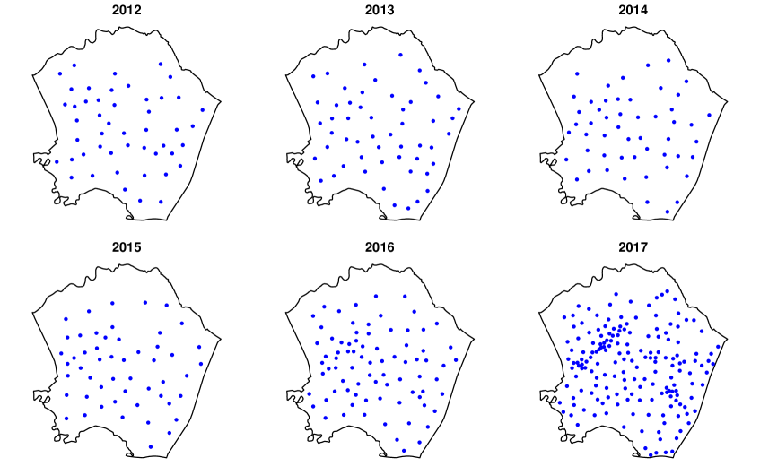
Figure 6 depicts the obtained barycenters, which except for the last pattern have cardinalities just slightly below the average weekly numbers of muggings of 51.7, 57.6, 52.8, 54.4, 82.5 and 196.9, respectively. The barycenters for the years 2012–2015 seem to be largely similar. Then in 2016 we start seeing patterns of denser structures forming along a line to the west and a center in the south-east of Kennedy. These can be actually identified as a main street and a major intersection in the densely populated parts of Kennedy.
6.2 Assault cases in Valencia
As a second application we analyze cases of assault in Valencia, Spain, reported to the police in the years 2010–2017. Since the addresses of the assaults and the street network are available, we treat this data as point patterns on a graph using shortest-path distance and . We acknowledge the local police in Valencia city together with the 112 emergency phone that kindly provided us the data after cleaning and removing any personal information.
We split up the graph and analyze the four central districts of Ciutat Vella, Eixample, Extramurs and El Pla del Real separately. For this we assigned each assault case to its district, but added also streets from other districts at the boundary, in order to enable more natural shortest-path computations. The north-south and east-west extensions of the districts vary roughly between 1.6 and 3.3 km.
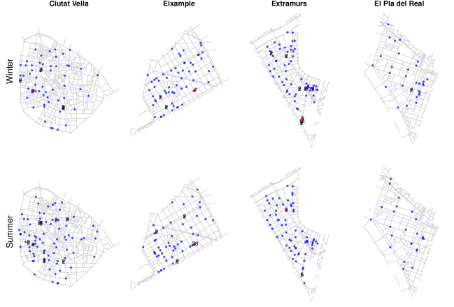
In the time domain we split up the assault data by year and season into seven winter patterns (data from December, January and February) and eight summer patterns (data from June, July and August), discarding for the present analysis data from the intermediate seasons, as well as from January and February 2010 and December 2017. We then computed barycenters per main season and district, obtaining “typical” assault patterns for summer and winter for each of the four districts considered, see Figure 7. The penalty was chosen as 800 m with respect to the shortest-path distance.
As mentioned in Subsection 4.1 when describing the subroutine optimBary that finds cluster centers on networks, we can calculate all distances that are relevant to the algorithm beforehand. For this we use the corresponding functionality built into the linnet objects in spatstat, which is very fast for the present purpose. On a standard laptop with a 1.6 GHz Intel i5 processor the computation took only about four seconds for the largest data set, which is Ciutat Vella in summer with a total of vertices (1676 street crossings plus 818 data points).
For the starting patterns in each district in summer and in winter, we chose random points, where ranged from times to times the median cardinality of the data point patterns. Since our present implementation of the kMeansBary algorithm on graphs runs without optimDelete and optimAdd steps, we based each barycenter on a large sample of starting patterns for each . This resulted in an overall total of calls to our algorithm for the eight scenarios, which on average took seconds each, using the precomputed distance matrices. One calculation in the largest setting (Ciutat Vella in summer) takes about seconds and in the smallest (El Pla del Real in summer) about seconds. The increase in the objective function was only up to 1% when decreasing the total number of calls to our algorithm by a factor of , resulting in a total computation time of well under one hour.
Due to the choice of it happens quite frequently that there are several optimal centers for some of the clusters obtained after convergence of the kMeansBary algorithm. In this case we take the average of their coordinates and project the result back onto the graph in order to obtain a somewhat more balanced result. The resulting point does not necessarily realize the same cluster cost as the original center points, but on a real street network it is not to be expected that the cost becomes considerably worse. In fact, for the data considered, the results hardly differed at all.
Figure 7 shows the barycenters for the different districts in winter and in summer. It seems that there are no very clear effects of the season on the assaults. In the first district (Ciutat Vella) there are substantially more assaults in summer, but their spatial distribution in the barycenter is more or less similar. In Eixample we see a concentration of assault cases in summer in the Barrio Ruzafa in the southern half of the district, whereas cases are more or less equally spread in winter. A notable feature is the occurrence of 23 barycenter points at a single crossing in summer and 7 points at the same crossing in winter with further points close by. This is due to the cul-de-sac visible in Figure 7, which in reality forms sort of a backyard that makes the area easy for assaults, especially in summer time when there are more people (especially tourists) moving around those parts of the city. The spot is well-known to the police and in recent years the number of assaults has decreased due to police interventions. The barycenters clearly reflect this (former) assault hot spot.
In the district of Extramurs both barycenters are more or less spread over the whole district, with two clusters of assaults occurring in the east and south. Both clusters are much more pronounced in winter. In the district of El Pla del Real there is some concentration in the winter month in the east and south-east. Apart from that the only noticeable difference is that there are substantially more assaults in winter than in summer, which may well be related to the fact that this is a popular student district.
7 Discussion and outlook
In this paper we have introduced the -th order TT- and RTT-metrics, which allow us to measure distances between point patterns in an intuitive way, generalizing several earlier metrics. We have investigated -th order barycenters with respect to the TT-metric and presented two variants of a heuristic algorithm. These variants return local minimizers of the Fréchet functional that mimic properties of the actual barycenter well and attain consistent objective function values. They are computable in a few seconds for medium-sized problems, such as 100 patterns of 100 points.
For the proof of Proposition 3.3 it was necessary to set . While such a choice may seem natural, we point out that due to the separate interpretations of as the order for matching points in the metric on (higher tends to balance out the matching distances) and as the order of the empirical moment in , it may well be desirable to combine .
In the present paper we have only dealt with the descriptive aspects of barycenters. It is thus clear that our applications in Section 6 can only be seen as explorative studies. In order to determine whether differences between group barycenters are statistically significant, we need to take the distribution of the point patterns around their barycenters into account and perform appropriate hypothesis tests.
Fortunately, the Fréchet functional (3.1) provides us with a natural quantification of scatter around the barycenter. For it is quite common to refer to
as (empirical) Fréchet variance, due to Equation (3.2). Detailed asymptotic theory for performing an analysis of variance (ANOVA) in metric spaces based on comparing Fréchet variances has been recently developed in Dubey and Müller, (2017). The application and adaptation of this theory for the point pattern space and an investigation of the performance of our heuristic algorithm in this context will be the subject of a future paper.
In a similar vein, a fast computation of reliable barycenters opens many doors to more advanced procedures in statistics and machine learning. This includes barycenter-based dimension reduction techniques, such as Wasserstein dictionary learning, see Schmitz et al., (2018), and functional principal component analysis of point patterns evolving in time, see Dubey and Müller, (2019).
Appendix: Proofs left out in the main text
Lemma A.1.
Let , and let be a metric space with . For set , where are pairwise different, and define
Then is a metric space.
Proof.
Identity and symmetry properties of the map follow immediately. Since is a metric on and is a metric on , we only have to check the triangle inequality for a few special cases. If and (or vice versa), then . Since one of and has to be regardless of , we obtain . If and , then
Likewise, if and , then
∎
Proof of Theorem 2.1.
Since , it is enough to show the statement for .
Let be a permutation that minimizes . Writing we obtain
| (A.1) |
Therefore, enumerating in arbitrary order as for some and setting for , we have
| (A.2) |
Thus .
Conversely, let minimize . This implies for all , because otherwise we could obtain a smaller value by removing , from the vector. Writing , it implies also that for all and , because otherwise we could obtain a smaller value by adding , to the vector. Let then be any permutation satisfying for all . With this we obtain exactly the -distances in (A.1) for all and hence (A.2) holds again. Thus . ∎
Proof of Proposition 2.3.
We start with the map . If , then and there is a permutation such that for . Hence , choosing and . If on the other hand , we must have to be able to achieve and there must be such that for . Since the is a metric, this yields . The symmetry of is immediately clear from the symmetric form of (2.1).
For the proof of the triangle inequality we use the metric space introduced before Theorem 2.1. Let . After filling up patterns to the maximum of the three cardinalities by adding points at the auxiliary location , we may assume that , and have the same cardinality. Noting that given two point patterns of the same cardinality we may add any number of extra points located at to both of them without changing their -distance, Theorem 2.1 yields that there are such that
Then matches the points of and in such a way that
and Theorem 2.1 and the triangle inequality for the -norm yields that
We turn to the map . Since , we may inherit the identity and symmetry properties for directly from . To show the triangle inequality, let , and be in and set . If , we obtain the desired result from the triangle inequality of as
If , we use a slightly different construction for the extended metric space. Let for two different . Setting
we obtain by Lemma A.1 that is again a metric space. Setting for and for , we may define and . Note that an optimal permutation for can be extended to an optimal permutation for by setting for . Furthermore, for any with , we have . Combining these two facts, we obtain
and therefore
where the second inequality holds since the cardinalities of all point patterns are equal and the equality holds by two more applications of Theorem 2.1. ∎
Proof of Proposition 2.4.
The equivalence for (a) was already used in Diez et al., (2012). We give a quick argument for the sake of completeness. We may assume without loss of generality that, in an admissible path for the minimization problem (2.3),
-
only moves from to occur;
-
only points are added;
-
only points are deleted;
because if any of these conditions were violated, the total cost of the path could only become larger (for the first item we use the triangle inequality for ). The minimization (2.3) is then equivalent to choosing points to be moved from -points with indices to -points with indices , respectively, at cost for each move. The remaining points of are deleted at cost per deletion, and the remaining points of are added at cost per addition. This yields exactly the minimization problem (2.1).
The equivalence (b) is an immediate consequence of Theorem 2.1. ∎
References
- Agueh and Carlier, (2011) Agueh, M. and Carlier, G. (2011). Barycenters in the Wasserstein space. SIAM J. Math. Analysis, 43:904–924.
- Anderes et al., (2016) Anderes, E., Borgwardt, S., and Miller, J. (2016). Discrete Wasserstein barycenters: optimal transport for discrete data. Math. Methods Oper. Res., 84(2):389–409.
- Baddeley et al., (2015) Baddeley, A., Rubak, E., and Turner, R. (2015). Spatial point patterns: methodology and applications with R. Chapman and Hall/CRC.
- Bandelt et al., (1994) Bandelt, H.-J., Crama, Y., and Spieksma, F. C. R. (1994). Approximation algorithms for multi-dimensional assignment problems with decomposable costs. Discrete Appl. Math., 49:25–50.
- Bertsekas, (1988) Bertsekas, D. P. (1988). The auction algorithm: A distributed relaxation method for the assignment problem. Annals of Operations Research, 14:105–123.
- Błaszczyszyn et al., (2018) Błaszczyszyn, B., Haenggi, M., Keeler, P., and Mukherjee, S. (2018). Stochastic geometry analysis of cellular networks. Cambridge University Press.
- Borgwardt and Patterson, (2018) Borgwardt, S. and Patterson, S. (2018). Improved linear programs for discrete barycenters. Preprint. https://arxiv.org/abs/1803.11313.
- Chiaraviglio et al., (2016) Chiaraviglio, L., Cuomo, F., Maisto, M., Gigli, A., Lorincz, J., Zhou, Y., Zhao, Z., Qi, C., and Zhang, H. (2016). What is the best spatial distribution to model base station density? A deep dive into two European mobile networks. IEEE Access, 4:1434–1443.
- Chizat, (2017) Chizat, L. (2017). Unbalanced Optimal Transport: Models, Numerical Methods, Applications. PhD thesis, PSL Research University.
- Chizat et al., (2018) Chizat, L., Peyré, G., Schmitzer, B., and Vialard, F.-X. (2018). Scaling algorithms for unbalanced optimal transport problems. Mathematics of Computation, 87(314):2563–2609.
- Cormen et al., (2009) Cormen, T. H., Leiserson, C. E., Rivest, R. L., and Stein, C. (2009). Introduction to Algorithms. MIT Press, Cambridge, MA, third edition.
- Cuturi and Doucet, (2014) Cuturi, M. and Doucet, A. (2014). Fast computation of Wasserstein barycenters. In Xing, E. P. and Jebara, T., editors, Proceedings of the 31st International Conference on Machine Learning, pages 685–693.
- del Barrio et al., (2019) del Barrio, E., Cuesta-Albertos, J. A., Matrán, C., and Mayo-Íscar, A. (2019). Robust clustering tools based on optimal transportation. Statistics and Computing, 29:139–160.
- Diez et al., (2012) Diez, D. M., Schoenberg, F. P., and Woody, C. D. (2012). Algorithms for computing spike time distance and point process prototypes with application to feline neuronal responses to acoustic stimuli. Journal of Neuroscience Methods, 203(1):186–192.
- Diggle, (2013) Diggle, P. J. (2013). Statistical analysis of spatial and spatio-temporal point patterns. Chapman and Hall/CRC.
- Dubey and Müller, (2017) Dubey, P. and Müller, H.-G. (2017). Fréchet analysis of variance for random objects. Preprint. https://arxiv.org/abs/1710.02761.
- Dubey and Müller, (2019) Dubey, P. and Müller, H.-G. (2019). Functional models for time-varying random objects. Preprint. https://arxiv.org/abs/1907.10829.
- Fréchet, (1948) Fréchet, M. (1948). Les éléments aléatoires de nature quelconque dans un espace distancié. Ann. Inst. H. Poincaré, 10:215–310.
- Hakimi, (1964) Hakimi, S. L. (1964). Optimum locations of switching centers and the absolute centers and medians of a graph. Operations Research, 12(3):456–458.
- Koliander et al., (2018) Koliander, G., Schuhmacher, D., and Hlawatsch, F. (2018). Rate-distortion theory of finite point processes. IEEE Transactions on Information Theory, 64(8):5832–5861.
- Konstantinoudis et al., (2019) Konstantinoudis, G., Schuhmacher, D., Ammann, R., Diesch, T., Kuehni, C., and Spycher, B. D. (2019). Bayesian spatial modelling of childhood cancer incidence in Switzerland using exact point data: A nationwide study during 1985–2015. Preprint. https://www.medrxiv.org/content/early/2019/07/15/19001545.
- Kuhn, (1955) Kuhn, H. W. (1955). The Hungarian method for the assignment problem. Naval Res. Logist. Quart., 2:83–97.
- Liero et al., (2018) Liero, M., Mielke, A., and Savaré, G. (2018). Optimal entropy-transport problems and a new Hellinger–Kantorovich distance between positive measures. Inventiones mathematicae, 211(3):969–1117.
- Lin and Müller, (2019) Lin, Z. and Müller, H.-G. (2019). Total variation regularized Fréchet regression for metric-space valued data. Preprint. https://arxiv.org/abs/1904.09647.
- Lombardo et al., (2018) Lombardo, L., Opitz, T., and Huser, R. (2018). Point process-based modeling of multiple debris flow landslides using INLA: an application to the 2009 Messina disaster. Stochastic environmental research and risk assessment, 32(7):2179–2198.
- Luenberger and Ye, (2008) Luenberger, D. G. and Ye, Y. (2008). Linear and nonlinear programming. Springer, New York, third edition.
- Mateu et al., (2015) Mateu, J., Schoenberg, F. P., Diez, D. M., Gonzáles, J. A., and Lu, W. (2015). On measures of dissimilarity between point patterns: Classification based on prototypes and multidimensional scaling. Biometrical Journal, 57(2):340–358.
- Moradi and Mateu, (2019) Moradi, M. and Mateu, J. (2019). First and second-order characteristics of spatio-temporal point processes on linear networks. Journal of Computational and Graphical Statistics, page to appear.
- Moradi et al., (2018) Moradi, M., Rodriguez-Cortes, F., and Mateu, J. (2018). On kernel-based intensity estimation of spatial point patterns on linear networks. Journal of Computational and Graphical Statistics, 27(2):302–311.
- Petersen and Müller, (2019) Petersen, A. and Müller, H.-G. (2019). Fréchet regression for random objects with Euclidean predictors. Annals of Statistics, 47(2):691–719.
- R Core Team, (2019) R Core Team (2019). R: A Language and Environment for Statistical Computing. R Foundation for Statistical Computing, Vienna, Austria.
- Rakshit et al., (2019) Rakshit, S., Davies, T., Moradi, M., McSwiggan, G., Nair, G., Mateu, J., and Baddeley, A. (2019). Fast kernel smoothing of point patterns on a large network using 2d convolution. International Statistical Review.
- Samartsidis et al., (2019) Samartsidis, P., Eickhoff, C. R., Eickhoff, S. B., Wager, T. D., Barrett, L. F., Atzil, S., Johnson, T. D., and Nichols, T. E. (2019). Bayesian log-Gaussian Cox process regression: applications to meta-analysis of neuroimaging working memory studies. Journal of the Royal Statistical Society: Series C, 68(1):217–234.
- Schmitz et al., (2018) Schmitz, M. A., Heitz, M., Bonneel, N., Ngole, F., Coeurjolly, D., Cuturi, M., Peyré, G., and Starck, J.-L. (2018). Wasserstein dictionary learning: Optimal transport-based unsupervised nonlinear dictionary learning. SIAM Journal on Imaging Sciences, 11(1):643–678.
- Schoenberg and Tranbarger, (2008) Schoenberg, F. P. and Tranbarger, K. E. (2008). Description of earthquake aftershock sequences using prototype point patterns. Environmetrics, 19(3):271–286.
- Schuhmacher, (2014) Schuhmacher, D. (2014). Stein’s method for approximating complex distributions, with a view towards point processes. In Schmidt, V., editor, Stochastic Geometry, Spatial Statistics and Random Fields, Vol. II: Models and Algorithms, pages 1–30. Springer. Lecture Notes in Mathematics 2120.
- Schuhmacher et al., (2008) Schuhmacher, D., Vo, B.-T., and Vo, B.-N. (2008). A consistent metric for performance evaluation of multi-object filters. IEEE Trans. Signal Processing, 56(8, part 1):3447–3457.
- Schuhmacher and Xia, (2008) Schuhmacher, D. and Xia, A. (2008). A new metric between distributions of point processes. Adv. in Appl. Probab., 40(3):651–672.
- Victor and Purpura, (1997) Victor, J. D. and Purpura, K. P. (1997). Metric-space analysis of spike trains: Theory, algorithms and application. Network: Comput. Neural Syst., 8:127–164.
- Weiszfeld, (1937) Weiszfeld, E. (1937). Sur le point pour lequel la somme des distances de points donnés est minimum. Tohoku Mathematical Journal, 43:355–386.