Chiral symmetry and Heun’s equation

Abstract

We show that the current quark mass should vanish to be consistent with the QCD color confinement: a bag model leads us to Heun’s equation, which requests that not only the energy but also the string tension should be quantized. This is due to the presence of higher order singularity which requests higher regularity condition demanding that parameters of the theory should be related to one another. As a result, the Hadron spectrum is consistent with the Regge trajectory only when quark mass vanishes. Therefore, in this model, the chiral symmetry is a consequence of the confinement.

1 Introduction

It has been understood that the QCD vacuum is working as a dual superconductor confining the color flux. As a consequence the Hadron spectrum is linear in quantum number $n$,

$$\alpha^{\prime}m^{2}=n+\beta,$$ (1)

which is the Regge trajectory that led to the discovery of the string theory. It is also known that chiral symmetry is one of the leading principle for the Hadron dynamics. For the chiral symmetry, the mass of the quarks should vanish at least approximately. Indeed, the current quark mass contribute less than 1% in counting the proton mass. However, little is understood why this should be so. In this paper, we will relate the vanishingly small quark mass to the Regge trajectory itself, which is a consequence of the confinement of the QCD color flux.

To show this, we will use a bag model which will lead us to the Heun’s differential equation(DE), which can be characterized by a DE with more than three singularities. The highest singularity at infinity and the one at 0, can be cancelled by factoring out two asymptotic behaviors. So if we have three singularities the left over singularity leads us two term recurrence relation and we can make the wave function normalizable by tuning the energy parameter such that the remaining factor of the wave function is truncated to a polynomial, which is the well known energy quantization.

Now if we have four or more singularities, then we need to tune two or more parameters of the differential equation to make the wave function normalizable. In terms of the Schrödinger equation, the result is rather dramatic: Not only the energy but also a parameter of the potential must be quantized. Sometimes, such extra quantization leads to obvious mismatch with the experimental data or well known principle unless some parameter vanishes. In our case, the spectrum of the hadron will be consistent with Regge trajectory only when the current quark mass vanishes. This result can be used to relate the origin of the chiral symmetry to QCD color confinement.

2 Quark-antiquark system with scalar interaction

To discuss the relation between the quark-mass and confinement, we use an old but simplest model where the confinement dynamics is captured as a Regge trajectory. Lichtenberg and collaborators[7] found a semi-relativistic Hamiltonian which leads to a Krolikowski type second order differential equation [8, 9, 10] in order to calculate meson and baryon masses in 1982. In the center-of-mass system, the relativistic expression for the total energy $H$ of two free particles of masses $m_{1}$, and $m_{2}$, and three-momentum $\vec{\mathbf{p}}$ is

$$H=\sqrt{\vec{\mathbf{p}}^{2}+m_{1}^{2}}+\sqrt{\vec{\mathbf{p}}^{2}+m_{2}^{2}}$$ (2)

Let $S$ be an interaction which is a Lorentz scalar and $V$ be an interaction which is a time component of a Lorentz vector. Then it is natural to incorporate the $V$ and $S$ into (2) by making the replacements

$$H\rightarrow H-V,\hskip 28.45274ptm_{i}\rightarrow m_{i}+\frac{1}{2}S,\qquad i=1,2.$$ (3)

Setting $m_{1}=m_{2}=m$, $V=0$ followed by (3), and introducing the scalar potential $S=br$, Gürsey et al. got a spin-free Hamiltonian for the meson ($q\bar{q}$) system [1, 2, 3, 4]:

$$H^{2}=4\left[(m+\frac{1}{2}br)^{2}+P_{r}^{2}+\frac{L(L+1)}{r^{2}}\right]$$ (4)

where we used $\vec{\mathbf{p}}^{2}=P_{r}^{2}+\frac{L(L+1)}{r^{2}}$ with $P_{r}^{2}=-\frac{\partial^{2}}{\partial r^{2}}-\frac{2}{r}\frac{\partial}{\partial r}$, and $L$ is the angular momentum and $b$ is real positive constant. Notice that the meaning of the linear scalar potential is to enforce the confinement of the quarks bound by a QCD flux string with constant string tension $b$. We will call the model simply a bag model afterward. For $m=0$, they could solve the eigenvalue problem $H^{2}\Psi=E^{2}\Psi$ and obtained energy eigenvalues

$$E^{2}=4b\left(L+N_{r}+3/2\right),$$ (5)

where $N_{r}=0,1,2,\cdots$ is the quantum number counting the radial nodes.

Notice that the energy is measured in the center of mass system therefore it is equal to the total mass of the system, namely the meson mass. Therefore above result is consistent with the Regge trajectories of slope $\frac{1}{4b}$. The purpose of this paper is to understand what happens in the case $m\neq 0$.

3 Heun’s equation

We start from the Schroedinger type equation $H^{2}\Psi=E^{2}\Psi$ with $H^{2}$ given by the Eq.(4), which can be considered as a non-relativistic Shcrödinger equation of the harmonic oscillator with extra linear potential apart from the usual quadratic potential.

Factoring out the asymptotic behaviors of wave function $\Psi$ near $r=0$ and $r=\infty$ by

$${\footnotesize\Psi(r)=\exp\left(-\frac{b}{4}\left(r+\frac{2m}{b}\right)^{2}\right)r^{L}y(r)Y_{L}^{M}(\theta,\phi)},$$ (6)

the differential equation for (4) becomes

$$r\frac{\partial^{2}{y}}{\partial{r}^{2}}+\left(-br^{2}-2mr+2(l+1)\right)\frac{\partial{y}}{\partial{r}}+\left(\left(\frac{E^{2}}{4}-b\left(L+\frac{3}{2}\right)\right)r-2m(L+1)\right)y=0$$ (7)

which is a bi-confluent Heun (BCH) equation whose canonical form is defined by

$$\rho\frac{d^{2}{y}}{d{\rho}^{2}}+\left(\mu\rho^{2}+\varepsilon\rho+\nu\right)\frac{d{y}}{d{\rho}}+\left(\Omega\rho+\varepsilon\omega\right)y=0$$ (8)

where $\mu$, $\varepsilon$, $\nu$, $\Omega$ and $\omega$ are real or imaginary parameters. It has a regular singularity at the origin and an irregular singularity at the infinity of rank 2 [5, 6].

Substituting $y(\rho)=\sum_{n=0}^{\infty}d_{n}\rho^{n}$ into (8), we obtain the following recurrence relation:

$$d_{n+1}=A_{n}\;d_{n}+B_{n}\;d_{n-1}\hskip 28.45274pt\quad\hbox{for }n\geq 1,$$ (9)

$$\hbox{\!\!where }A_{n}=-\frac{\varepsilon(n+\omega)}{(n+1)(n+\nu)},\quad B_{n}=-\frac{\Omega+\mu(n-1)}{(n+1)(n+\nu)},$$ (10)

and $d_{1}=A_{0}d_{0}$ for $n=0$. Comparing (7) with (8), the former is a special case of the latter with $\mu=-b$, $\varepsilon=-2m$, $\nu=2(L+1)$, $\omega=L+1$ and

$$\Omega=E^{2}/4-b(L+3/2).$$ (11)

Unless $y(\rho)$ is a polynomial, $\Psi$ is divergent as $\rho\rightarrow\infty$.

4 Normalizable solutions for the modified BCH equation

It has been believed that we can make the wave function normalizable whatever form is the Schroeding equation by tuning the energy eigenvalue. However, what we shall meet is the fact that we need to fine tune one more parameter apart from the energy in order to build normalizable (polynomial) solution for the Heun equations. This is because their series expansions consist of a three term recurrence relation given in Eq.(9) even after we factored out asymptotic behavior. Notice, on the other hand, hypergeometric-type functions gives only two term recursive relations, in which case we can construct normalizable polynomial solution by tuning the single parameter, energy. Actually, the necessary and sufficient condition for constructing polynomials with a single parameter is that its power series should be reduced to the two term recurrence relation. For the Heun equation case, we cannot reduce its recursive relation to the two term case. We can build polynomials by fine tuning two parameters, for example, $b$ and $E^{2}$.

For polynomials of (7) around $r=0$, we treat $m$ as a free variable; consider $-\Omega/\mu=E^{2}/4b-(L+3/2)$ to be a positive integer; and treat $b$ as a fixed value. Through (9), we are able to see that a series expansion becomes a polynomial of degree $N$ if we impose two conditions

$$B_{N+1}=d_{N+1}=0\hskip 28.45274pt\hbox{ for some }\;N\in\mathbb{N}_{0}$$ (12)

Eq. (12) is sufficient to give $d_{N+2}=d_{N+3}=d_{N+4}=\cdots=0$ successively and the solution to eq.(7) becomes a polynomial of order $N$.

To see what is going on we follow a few low order process.
For $N=0$, Eq.(12) gives $B_{1}=\frac{-\Omega}{2(2L+3)}=0$ and $d_{1}=A_{0}d_{0}=md_{0}=0$. If we choose $d_{0}=0$ the whole series solution vanishes. Therefore there is no solution unless $m=0$, in which case the solution is reduced to that of the Hypergeometric case with $E^{2}=4b(L+3/2)$. Since we are considering the case $m\neq 0$, we conclude that there is no solution with radial nodal number $N=0$.

For $N=1$, $B_{2}=\frac{-\Omega+b}{3(2L+4)}$ and $d_{2}=A_{1}d_{1}+B_{1}d_{0}=(A_{0}A_{1}+B_{1})d_{0}=\left(\frac{4m^{2}(L+1)(L+2)}{2(2L+2)(2L+3)}-\frac{b}{2(2L+3)}\right)d_{0}$. Requesting both $B_{2}$ and $d_{2}$ to be zero, we get $b=2m^{2}(L+2)$ and $E^{2}=4b(L+1+3/2)=8m^{2}(L+2)(L+5/2)$ with $L=0,1,2,\cdots$. In this case, $y(\rho)=\sum_{n=0}^{1}d_{n}\rho^{n}=1+m\rho$ where $d_{0}=1$ chosen for simplicity from now on. Since N=0 is not allowed for $m\neq 0$, $N=1$ is the case containing the ground state.

For $N=2$, we have $B_{3}=\frac{-\Omega+2b}{4(2L+5)}$ and $d_{3}=A_{2}d_{2}+B_{2}d_{1}=\left(\frac{2(L+2)(L+3)m^{3}}{3(2L+3)(2L+4)}-\frac{2(L+3)mb}{3(2L+3)(2L+4)}-\frac{mb}{3(2L+4)}\right)d_{0}$. So, the Eq.(12) gives $b=\frac{2m^{2}(L+2)(L+3)}{4L+9}$ and $E^{2}=\frac{8m^{2}(L+2)(L+3)(L+7/2)}{4L+9}$ with $L=0,1,2,\cdots$. Its eigenfunction is $y(\rho)=\sum_{n=0}^{2}d_{n}\rho^{n}=1+m\rho+\frac{L+2}{4L+9}m^{2}\rho^{2}$.

For larger $N$, the energy eigenvalue is determined from $B_{N+1}=0$, or equivalently $\Omega=-\mu N=bN$. Eq.(11) gives

$$E^{2}=4b\left(N+L+\frac{3}{2}\right),$$ (13)

with $L=0,1,2,\cdots,N$. Allowed values of $b$’s are obtained from $d_{N+1}=0$, which are quantized. Its eigenfunction is $N$-th order polynomial

$$y_{N}(\rho)=1+m\rho+\sum_{i=2}^{N}d_{i}\rho^{i}.$$ (14)

5 Necessity of extra quantization

We observed that both $E$ and $b$ are quantized in order to have a polynomial solution (14) when we have three term recurrence relation. However, for many people including the authors, it is not easy to accept the idea that one more parameter other than the energy should be quantized. The question of extra quantization is equivalent to asking whether imposing both conditions in Eq.(12) are the only way to get the normalizable solution, although it is clear that they are sufficient.

Here we demonstrate numerically that we can not construct a normalizable solution of the BCH equation by tuning only $E^{2}$ using the shooting method. Let $m=1$ and $L=0$ in (7) for simplicity. According to previous section, the ground state for $m\neq 1$ happened at $N=1$ with $E^{2}=E_{0}=40$, but $b=b_{0}=4$ was also required. In this case polynomial was given by $1+r$. What will happen if we do not request quantizing $b$?

Let $b$ is different from the quantized value $b_{0}$ so that $b=b_{0}+1.0$. We look for a proper value of $E^{2}$ with initial conditions $y(0)=d_{0}=1,y^{\prime}(0)=d_{1}=m=1$. Then we try to construct a normalizable solution by shooting method.

(1)	$E^{2}=E_{0}+7.496817$
(2)	$E^{2}=E_{0}+7.496818$
(3)	$E^{2}=E_{0}+7.49681789$
(4)	$E^{2}=E_{0}+7.49681790$
(5)	$E^{2}=E_{0}+7.4968178907$
(6)	$E^{2}=E_{0}+7.4968178908$
(7)	$E^{2}=E_{0}+7.496817890781$
(8)	$E^{2}=E_{0}+7.496817890782$
(9)	$E^{2}=E_{0}+7.4968178907817$
(10)	$E^{2}=E_{0}+7.4968178907818$
(11)	$E^{2}=E_{0}+7.49681789078176$
(12)	$E^{2}=E_{0}+7.49681789078177$
(13)	$E^{2}=E_{0}+7.496817890781766$
(14)	$E^{2}=E_{0}+7.496817890781767$
(15)	$E^{2}=E_{0}+7.4968178907817661$
(16)	$E^{2}=E_{0}+7.4968178907817662$

Table 1: $E^{2}$ of $y(r)$ for $b=b_{0}+1.0$.
See Fig. 2

.

(1)	$E^{2}=E_{0}-10^{-6}$
(2)	$E^{2}=E_{0}+10^{-6}$
(3)	$E^{2}=E_{0}-10^{-8}$
(4)	$E^{2}=E_{0}+10^{-8}$
(5)	$E^{2}=E_{0}-10^{-10}$
(6)	$E^{2}=E_{0}+10^{-10}$
(7)	$E^{2}=E_{0}-10^{-12}$
(8)	$E^{2}=E_{0}+10^{-12}$
(9)	$E^{2}=E_{0}-10^{-13}$
(10)	$E^{2}=E_{0}+10^{-13}$
(11)	$E^{2}=E_{0}-10^{-14}$
(12)	$E^{2}=E_{0}+10^{-14}$
(13)	$E^{2}=E_{0}-10^{-15}$
(14)	$E^{2}=E_{0}+10^{-15}$
(15)	$E^{2}=E_{0}-10^{-16}$
(16)	$E^{2}=E_{0}+10^{-16}$

Table 2: $E^{2}$ of $y(r)$ for $b=b_{0}$.
See Fig. 2

.

In Fig. 2 shows how the trial wave functions approach to $1+r$ as we increase the precision of the eigenvalue $E^{2}$. The odd numbered solutions (1),(2), … are undershooted ones and even numbered ones are overshooted ones. Starting from a under-shooted solution, one can increase the precision of the eigenvalue $E^{2}$ by increasing minimal amount in the next digit to get the over-shooted solution. Similarly, starting from a over-shooted solution one can increase the precision of the eigenvalue by decreasing minimal amount in the next digit to get the under-shooted solution. After a number of iterations, the solutions stop to approach to $1+r$ although we increase the precision by alternating the over- and under-shooting. This can be seen from the Fig. 2: there is a limit to pushing the solution to the right as we see from overlapped solutions (11), (13), (15), and (12), (14), (16). When $E^{2}$ reaches around $E_{0}+7.49681789078176$, $y(r)$ starts to be flipped violently without moving to the right any more.

This should be contrasted with $b=b_{0}$ case shown in Fig. 2 where the solution $y(r)$ is pushed to the right as $E^{2}$ approaches 40 with $b=b_{0}=4$ without problem. And we can easily check that if $E^{2}$ is exactly 40, $y(r)=1+r$ numerically also.

Above demonstration help us to accept necessity of two quantized parameters ($E^{2}$ and $b$) to create a polynomial, when a series solution of (7) have of a three term recurrence relation.

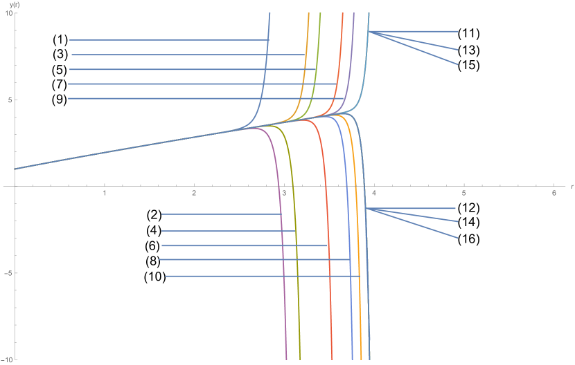
Figure 1: $y(r)$ with a fixed $b=b_{0}+1.0$ and unfixed $E^{2}$’s as $m=1$

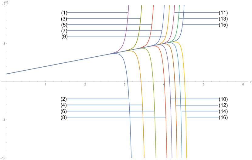
Figure 2: $y(r)$ with a fixed $b=b_{0}$ and unfixed $E^{2}$’s as $m=1$

6 Quantization of $b$

Once we are convinced that both $E$ and $b$ are quantized, we will find what are the available quantized values of $b$ for higher orders in the case of a decrease in energy level. For $N=L=10$, there are 5 possible real values of $b/m^{2}$: 0.366018, 0.579236, 1.03967, 2.35494 and 9.45702. We choose the biggest real roots of $b/m^{2}$ in each case because it minimizes energy loss in a decrease in energy level: Also, the biggest one makes $E_{1}<E_{3}<E_{5}<\cdots$ and $E_{2}<E_{4}<E_{6}<\cdots$, here, $E_{i}$ is the $i^{th}$ excited eigenvalue.

Fig. 3 shows us the biggest real values of $b/m^{2}$ with given odd $N$ and $L$. There are $(N+1)/2$ of $b/m^{2}$ corresponding to each $L=0,1,2,\cdots$. In each $N$, the lowest point is the numeric value of $b/m^{2}$ for $L=0$; the next point is for $L=1$; the top point is for $L=21$. We observe that $b/m^{2}$ increases as $N$ increases with fixed $L$. As $N\rightarrow\infty$, $b/m^{2}$ goes to infinity for any fixed $L$. Figs. 3 shows us that the gap between two successive points is constant with given $N$ as $L$ increases. Similarly, we find that the biggest real values of $b/m^{2}$ with given even $N$ and $L$ is 1/4 less than the biggest real ones with odd $N$ and $L$.

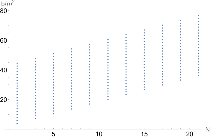
Figure 3: Real values of $b/m^{2}$’s for $N=1,3,5,\cdots$ & $L=0,1,2,\cdots,N$.

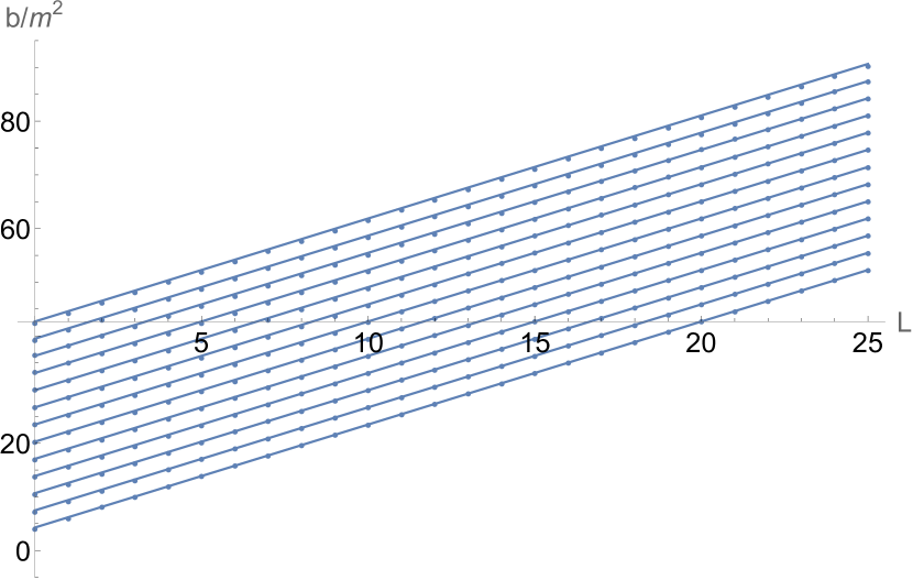
Figure 4: Fitting of $b/m^{2}$ by eq.(15) as functions of $L$ with odd $N$.

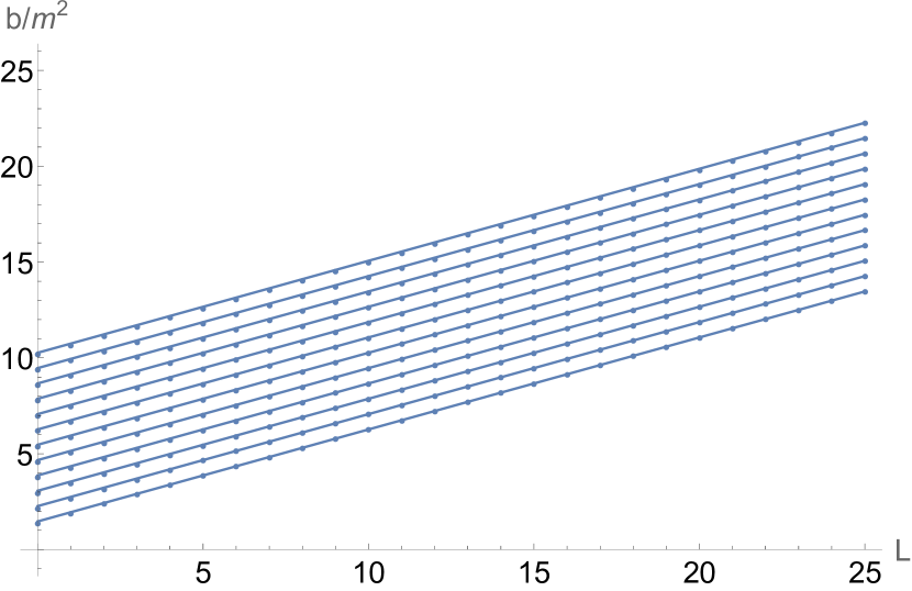
Figure 5: Fitting of $b/m^{2}$ by eq.(16) as functions of $L$ with even $N$.

For odd $N$, Fig. 4 shows us that the allowed value of $b/m^{2}$ is linear in $L$ and can be approximated by the rational function

$$\frac{b}{m^{2}}=\frac{8}{5}\left(N+\frac{6}{5}L+\frac{5}{3}\right)$$ (15)

. For the figure, we calculated 625 different values of $b/m^{2}$’s at various $(N,L)$. The lowest fit line is for $N=1$, the top one which has the most steep slop is for $N=25$.

For even $N$, Fig. 5 shows us that the allowed value of $b/m^{2}$ is also linear in $L$ and can be approximated

$$\frac{b}{m^{2}}=\frac{2}{5}\left(N+\frac{6}{5}L+\frac{5}{3}\right)$$ (16)

.

By substituting eq.(15) and eq.(16) into eq.(13), we get the experimental fit to the eigenvalue $E^{2}$:

For odd $N$,

$$E^{2}\approx\frac{32}{5}\left(N+\frac{6}{5}L+\frac{5}{3}\right)\left(N+L+\frac{3}{2}\right)m^{2}$$ (17)

For even $N$,

$$E^{2}\approx\frac{8}{5}\left(N+\frac{6}{5}L+\frac{5}{3}\right)\left(N+L+\frac{3}{2}\right)m^{2}$$ (18)

One obvious consequence of our analysis is that the mass spectrum which is roughly given by Eq.(17) and Eq.(18) can not be linear in $N$ unlike $m=0$ case given in Eq.(5). This is attributed to the fact that higher order singularity of the differential equation requests higher regularity condition so that $b$ should be determined by other parameters, which in turn introduces extra dependence of $E^{2}$ on $N$ and $L$ through that of $b$.

7 Conclusion

In this paper, we considered the spectrum of a bag model with non-zero quark mass, and found that the mass of the hadrons are non-linear, while it is linear if the quark mass is zero. In the model given by Eq.(4), the presence of current quark mass introduces a higher order singularity which requires extra regularity condition so that the string tension $b$ must be related to the other parameter of the model and should be quantized. As a result, $b$ gets extra $N$ dependence and the spectrum becomes non linear, which is inconsistent with the Regge trajectory that is tied with the color confinement. In this sense and context, we can say that chiral symmetry is induced by the color confinement. It would be interesting if similar argument can be done in other approach of hadrons.

References

- [1] Catto, S. and Gürsey, F., “Algebraic treatment of effective supersymmetry,” Nuovo Cim. 86A. (1985)201.
- [2] Catto, S. and Gürsey, F., “New realizations of hadronic supersymmetry,” Nuovo Cim. 99A, (1985)685.
- [3] Catto, S., Cheung, H. Y., Gursey, F., “Effective Hamiltonian of the relativistic Quark model,” Mod. Phys. Lett. A 38, (1991)3485.
- [4] Gürsey, F., Comments on hardronic mass formulae, in A. Das., ed., From Symmetries to Strings: Forty Years of Rochester Conferences, World Scientific, Singapore, (1990).
- [5] NIST Digital Library of Mathematical Functions, “Confluent Forms of Heun Equation,” http://dlmf.nist.gov/31.12
- [6] Slavyanov, S. Yu., Lay W. Special Functions: A Unified Theory Based on Singularities, Oxford Mathematical Monographs, Oxford University Press, Oxford, (2000).
- [7] Lichtenberg, D. B., Namgung, W., Predazzi, E. and Wills,J. G., “Baryon masses in a relativistic quark-diquark model,” Phys. Lett. 48, 1653(1982).
- [8] Krolikowski, W., “Relativistic three-body equation for one Dirac and two Klein-Gordon particles,” Acta Phys. Pol. B. 11(5), 387–391(1980).
- [9] Krolikowski, W., “Solving nonperturbatively the breit equation for parapositronium,” Acta Phys. Pol. B. 12(9), 891–895(1980).
- [10] Todorov, I. T., “Quasipotential Equation Corresponding to the Relativistic Eikonal Approximation,” Phys. Rev. D3, 2351(1971)