Quasi-simultons in thermal atomic vapors

Abstract

The propagation of two-color laser fields through optically thick atomic ensembles is studied. We demonstrate how the interaction between these two fields spawns the formation of co-propagating, two-color soliton-like pulses akin to the simultons found by Konopnicki and Eberly [Phys. Rev. A 24, 2567 (1981)]. For the particular case of thermal Rb atoms, exposed to a combination of a weak cw laser field resonant on the D1 transition and a strong, sub-ns laser pulse resonant on the D2 transition, simulton formation is initiated by an interplay between the 5s_1/2 – 5p_1/2 and 5s_1/2 – 5p_3/2 coherences which amplifies the D1 field at the arrival of the D2 pulse producing sech-squared pulse with a length of less than 10 microns. This amplification is demonstrated in a time-resolved measurement of the light transmitted through a thin thermal cell. We find good agreement between experiment and a model that includes the hyperfine structure of the relevant levels. With the addition of Rydberg dressing, quasi-simultons offer interesting prospects for strong photon-photon interactions in a robust environment.

Self-induced transparency manifests dramatically by the formation of optical solitons propagating undistorted over long distances in a medium opaque to a cw field of the same wavelength McCall . A short light pulse may propagate as a soliton or split into multiple solitons only if it is sufficiently intense area . However, it has been known for some time that a weak soliton-like pulse at one frequency can co-propagate with a stronger soliton-like pulse at another frequency. Solutions of the Maxwell-Bloch equations describing this situation in doubly resonant 3-level V-systems were first found in the form of matched sech pulses, or simultons, under the condition that the two transitions have the same oscillator strength Kono81 ; seealso . Remarkably, the two pulses may co-propagate as a simulton even if neither of them is strong enough to support a soliton in the absence of the other field Rahman . The condition that the two transitions have the same oscillator strength is difficult to realize experimentally othersystems but makes the Maxwell-Bloch equations integrable in the sense of the inverse scattering transform (in a suitable approximation), which permits an in depth analysis of their analytical solutions multisimultons .

However, this condition can be relaxed without compromising the formation of pairs of soliton-like pulses co-propagating with little distortion over much longer distances than allowed by Beer’s law Bolshov85 ; Bolshov88 . We refer to such pairs of pulses as quasi-simultons, to distinguish them from the ideal sech-simultons of Ref. Kono81 . It has been noted, in particular, that a soliton on one transition of a V-system may enhance transmission of a weak pulse on the other transition even if the latter has a different oscillator strength Kozlov98 . The soliton may amplify the weak pulse and transport it through the medium simulton-like KozlovandKozlova2009 ; KK2010 . The term soliton-induced transparency has been coined for this effect KozlovandKozlova2009 . To our knowledge, it has previously been observed only in the propagation of superradiance pulses in a neon plasma Denisova98 .

In this paper, we show that soliton-induced transparency is readily seen in experiments using thermal vapor cells, in our case a thin cell containing a rubidium vapor cell ; james addressed by a cw field resonant on the D1 transition and a pulsed field resonant on the D2 transition. The numerical simulations described below reproduce the observed increase in transmission and pulse shaping indicating that this change signals the formation of a quasi-simulton.

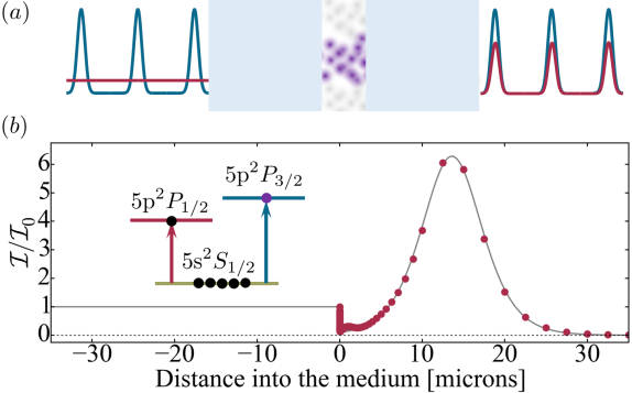
Figure 1: (color online) (a) Schematic of the experiment (not to scale). A cw probe field (red) resonant with the 5s${}_{1/2}(F=3)$ – 5p${}_{1/2}(F=3)$ transition of ⁸⁵Rb co-propagates with a pulsed coupling field (blue) resonant with the 5s${}_{1/2}(F=3)$ – 5p${}_{3/2}(F=4)$ transition. These two beams are focused to a waist of order 10 $\mu$m inside a 2 $\mu$m vapor cell containing Rb. (b) Inset: The level scheme indicating the probe and coupling fields. Main plot: Snapshot of the intensity of the probe field inside the medium, relative to the incident intensity, taken 0.05 ns after the coupling pulse reached its maximum at the front of the medium; the circles are calculated points and the solid line is a fit of these with a sech-squared pulse of width 8.6 $\mu$m (fwhm).

A sketch of the experiment is shown in Fig. 1(a). A dense, 2-$\mu$m thick thermal vapor of rubidium atoms in their natural isotopic abundances interacts with two co-propagating monochromatic laser beams forming a V-type excitation scheme. The probe and coupling beams are linearly polarized in orthogonal directions. They are resonant on, respectively, the $5{\rm s}_{1/2}(F=3)$ – $5{\rm p}_{1/2}(F=3)$ and $5{\rm s}_{1/2}(F=3)$ – $5{\rm p}_{3/2}(F=4)$ transitions of ⁸⁵Rb. The coupling beam is focused to a waist of $\sim\!20~{}\mu\mathrm{m}$ while the probe beam is focused more tightly to a waist of $\sim\!10~{}\mu\mathrm{m}$, which minimizes variation of the coupling intensity for the atoms in the probe beam. The probe field applied to the cell is cw. The coupling field is shaped to a short, nearly Gaussian pulse of a duration of typically 0.8 ns full width at half maximum (fwhm). Taking losses into account, we estimate that at the front of the medium, and on axis, the coupling field had an intensity of 3.7 kW cm^-2 at a measured peak power of 85 mW and the probe field an intensity of 24 W cm^-2. Following propagation the two fields are separated by a polarizing beam splitter and their transmission through the medium is monitored using a fast photodiode Supplemental ; Scully . The temporal variation of the measured probe field for various peak powers of the coupling pulse is shown in Fig. 2(a). The main feature of these data is a strong increase in transmission on the raising edge of the coupling pulse.

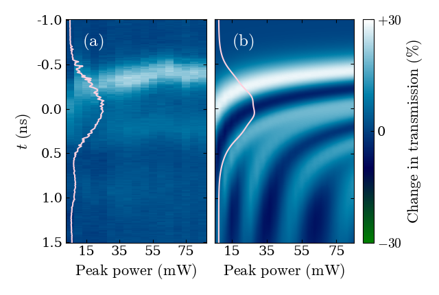
Figure 2: (color online) The change in the transmission at the probe frequency for a 2 $\mu$m-long Rb vapor relative to the average transmission at $t<-1$ ns, vs. the peak power of the incident coupling pulse. The pink curves represent the temporal intensity profile of the latter, at the back of the medium, for an initial peak power of 85 mW. The zero of the color scale corresponds to no change compared to the transmission before the arrival of the coupling pulse. The temperature is 200^∘C. (a): As measured. (b): As predicted by the model described in the text.

The other panel of this figure shows the results predicted by a model described below. Before addressing these, we first consider a simplified model consisting of a single ground state (state 0) resonantly coupled to a first excited state by a weak field (the probe field) and to a second excited state by a strong pulse (the coupling field) [Fig. 1(b)]. We take the coupling field at the front of the medium to be a Gaussian pulse of 1 kW cm^-2 peak intensity and 0.8 ns duration (fwhm in intensity), and the probe field to have an initial constant intensity of 10 $\mu$W cm^-2. We set the excited states lifetimes and the transition wavelengths and dipole moments to values corresponding to the D1 and D2 lines of ⁸⁵Rb, respectively. The oscillator strengths of the two transitions thus differ by a factor of 2 here. We neglect Doppler broadening, self-broadening and the hyperfine structure of the states for the time being. We assume 1D propagation transverse , make the rotating wave and slowly varying envelope approximations, and solve the resulting Maxwell-Bloch equations numerically, taking the atoms to be initially in the steady state driven by the probe field.

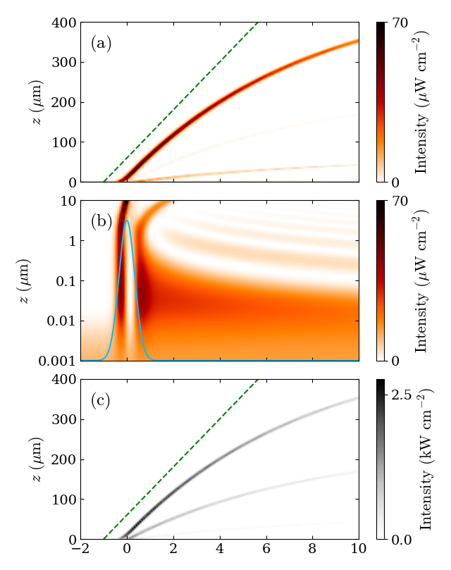
Figure 3: (color online) Formation of quasi-simultons in a 3-state model of an isotopically pure ⁸⁵Rb vapor, neglecting Doppler broadening and self-broadening. The atomic density corresponds to a temperature of 220^∘C. (a): The intensity of the probe field vs. time and propagation distance within the medium. This field is resonant on the D1 transition and has a constant intensity of 10 $\mu$W cm^-2 at the entrance of the medium ($z=0$). The 0.8-ns coupling pulse is resonant on the D2 transition and has a peak intensity of 1 kW cm^-2 at $(t=0,z=0)$. The dashed green line indicates the trajectory which a pulse propagating at a constant speed of $2\times 10^{-4}\;c$ would trace in the figure. (b): Enlargement of the small-$z$ region of panel (a). The blue curve represents the temporal profile of the coupling pulse (the intensity scale is arbitrary). (c): The same as (a) but for the coupling field.

Fig. 1(b) and Fig. 3 show how the probe and coupling fields vary both in space and in time within this 3-state model. Figs. 3(a) and (b) refer to the probe field. As seen from these figures, this field practically vanishes as soon as it enter the medium, prior to the arrival of the coupling pulse (the attenuation is extremely fast because the field is resonant with the transition and Doppler broadening is neglected). However, the arrival of that pulse triggers a more complicated dynamics. Microscopically, the onset of this dynamics can be traced to a rapid increase of the $\rho_{12}$ coherence. This increase, in turns, produces a large variation and a change of sign of the $\rho_{01}$ coherence, leading to an amplification of the probe field without a population inversion between the ground state and the first excited state Kozlov98 ; Denisova98 . In particular, the probe field develops into three successive pulses penetrating far deeper into the medium than the initial cw field. As shown in Fig. 3(a), these three pulses propagate soliton-like over many tens of micrometers, each at a different speed (the second of these three pulses is almost invisible in the figure). The first one is the fastest, although its maximum speed is only about $2\times 10^{-4}\,c$. It is also the strongest, and at its peak reaches an intensity larger than that of the incident cw field by almost a factor of 7. Like the other two, it becomes weaker and slower as it propagates. A snapshot of the spatial profile of the probe field at a time when this first pulse has just formed is shown in Fig. 1(b). The strong spatial localization of this pulse caused by the slow light effect is worth noting, as is its almost pure sech² profile.

The 0.8 ns coupling pulse also splits into three soliton-like pulses; the first and second ones are well visible in Fig. 3(c), but not the third one. This pulse is strong enough to break into three solitons even in the absence of the probe field. The presence of the latter does not affect the propagation of the coupling field significantly, but each of these three solitons co-propagates with a pulse at the probe frequency, thereby forming three quasi-simultons.

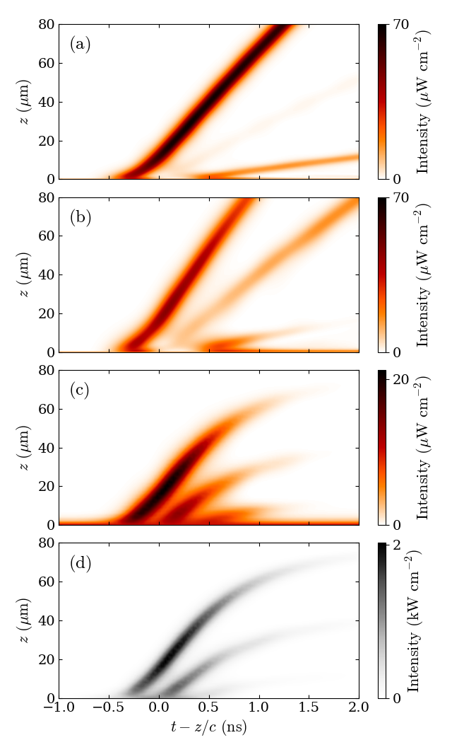
Figure 4: (color online) (a): The intensity of the probe field in the 3-state model of Fig. 3. This part of the figure is an enlargement of the small $|t-z/c|$, small $z$ region of Fig. 3(b). (b): The same as (a) but with the full hyperfine structure of the 5s_1/2, 5p_1/2 and 5p_3/2 states included in the calculation. (c): The same as (b) but now also including Doppler broadening and self-broadening. (d): The same as (c) but for the coupling field.

Differences in transition dipole moments between the magnetic substates coupled to each other by the two fields may compromise the formation of simultons when the relevant levels have a hyperfine structure. However, this issue is not of major importance here because the bandwidth of the coupling pulse is sufficiently large compared to the energy splitting between the relevant hyperfine states fewcycle . Fig. 4 compares the predictions of the 3-state model, in (a), to the results obtained when the complete hyperfine structure of the relevant levels is included in the calculation, in (b). While there are differences between these two sets of results, it is clear that in the present case the hyperfine structure does not prevent the formation of quasi-simultons and their propagation over a considerable distance. However, the hyperfine structure of the 5s and 5p levels is an important issue for longer coupling pulses Supplemental ; magneticfield .

We now include not only the hyperfine structure but also Doppler broadening and self-broadening. The corresponding results are shown in panels (c) and (d) of Fig. 4. Quasi-simultons are still found in these more complete calculations. Although not as stable, they still propagate over far longer distances than would be the case for weak cw fields of the same wavelengths, and the probe field is still amplified through its interaction with the coupling pulse.

We used the same model as in Figs. 4(c) and (d) to obtain the results displayed in Fig. 2(b), except that we assumed the incident probe field had the same (much higher) intensity as in the experiment. We ignored the transverse Gaussian profiles of the laser beam, as factoring these in would have led to excessively long computations. Interaction with the windows was taken into account by broadening each state by 30 MHz JamesThesis . Comparing Fig. 2(b) to Fig. 2(a), we see that the model does not predict the rapid damping of the dynamics which follows the initial increase in transmission on the raising edge of the coupling pulse (the origin of this damping as yet unknown). However, it reproduces this strong increase well.

We also ran this calculation for a 50 $\mu$m-long cell, so as to see how this increase in the transmission develops over longer propagation distances (Fig. 5). Taking pulse re-shaping into account would be necessary for comparing to measurements for a cell of that length; however, here we only aim at illustrating how the 1D dynamics would evolve beyond 2 $\mu$m if it was remaining unperturbed. As seen from the figure, this enhancement would develop into a well defined pulse co-propagating with the first of the solitons the coupling pulse splits into. It can thus be identified with the formation of a quasi-simulton.

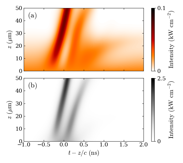
Figure 5: (color online) (a) The calculated probe field for the conditions of Fig. 2, now for a much longer propagation distance of 50 $\mu$m. The peak power of the coupling pulse is 35 mW. (b) The corresponding coupling field.

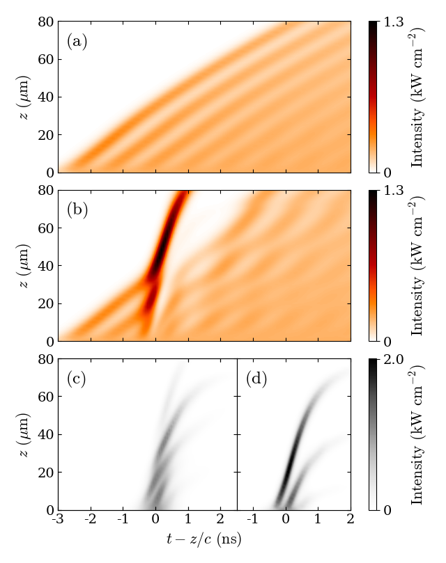
Figure 6: (color online) (a) The probe field in the absence of a coupling pulse, assuming that at $z=0$ this field is a flat-top pulse smoothly turned on from 0 to 200 W cm^-2 between $t=-5$ and $t=-2$ ns. As in Fig. 4(c), the model includes Doppler and self-broadening as well as the full hyperfine structure of the 5s and 5p energy levels. (b) The same as (a) but here assuming an incident 0.8 ns coupling pulse of 1 kW cm^-2 peak intensity. (c): The coupling field corresponding to the probe field shown in (b). (d): The same as (c) but assuming an incident intensity of only 10 $\mu$W cm² at the probe frequency, instead of 200 W cm^-2.

It is interesting to explore this dynamics for still higher intensities of the probe field. To avoid strong optical pumping, we now assume that the probe field at the entrance of the medium is a flat-top pulse turned on over 3 ns. Taking the intensity after turn on to be 200 W cm^-2 yields the results shown in panels (a), (b) and (c) of Fig. 6. Panel (a) shows the probe field in the absence of a coupling pulse: at this high intensity, the incident flat-top pulse splits into a periodic train of soliton-like pulses upon entering the medium. Adding a strong coupling pulse perturbs this dynamics considerably, as shown in panel (b). In particular, we note the formation and amplification of a strong pulse at the probe frequency associated with the pulse at the coupling frequency. However, the latter [panel (c)] is now strongly affected by its interaction with the former, contrary to what is found at lower intensities of the probe field [compare Fig. 6(c) to Fig. 6(d), which shows the coupling field found when the probe intensity at $z=0$ is only 10 $\mu$W cm^-2 after turn on].

In conclusion, we have demonstrated the amplification of a weak probe field by a strong pulse — the first step in the formation of quasi-simultons. Such simultons allow the propagation of weak localised fields through optical thick media. The satisfactory agreement between theory and experiment found in Fig. 2 shows the applicability of our model, extended as necessary, to the exploration of what other two-color propagation phenomena could be observed in thermal atomic vapors. Future work will include investigating the single photon regime, the potential of Rydberg dressing rydberg to induce strong photon-photon interaction, and the possibility of photon crystals.

SUPPLEMENTAL MATERIAL

Method

Experiment

As is explained in the paper, the experimental setup involves two laser beams (the probe beam and the coupling beam) co-propagating through a thin cell containing a Rb vapor.

The probe beam is first split by a polarizing beam-splitter cube (PBSC). Part of it is sent to a HighFinesse WS-7 wavemeter, resolution 0.1 pm. The wavelength is monitored through the latter and controlled by a LABVIEW program locking the probe laser to the 5s${}_{1/2}(F=3)$ – 5p${}_{1/2}(F=3)$ transition of ⁸⁵Rb. The rest of the beam is sent to the cell.

The coupling beam is also first split by a PBSC. The split beam is used to lock the laser on the 5s${}_{1/2}(F=3)$ – 5p${}_{3/2}(F=4)$ transition by polarization spectroscopy Pearman . The rest of the coupling beam is sent to a Pockels cell immediately preceded and immediately followed by crossed Glan-Taylor PBSCs with an extinction ratio exceeding $10^{5}$. This very high extinction ratio results in negligible beam power transmitted through the Pockells cell when it is not activated. This cell is connected to an electric pulse generator producing an approximately Gaussian pulse with a fwhm of 0.8 ns. The temporal profile of the light pulse so generated is recorded using a single-photon counting module.

The two beams have orthogonal linear polarizations, so that they can be separated with a PBSC after the cell. In addition to this polarization filter (extinction $\sim$ 200), we use a Semrock FF01-800/12 bandpass filter passing 795 nm light with 95% transmission and blocking 780 nm light with a measured extinction of $3.5\times 10^{3}$. This setup ensures that there is no detectable probe signal when the 780 nm coupling beam is on with the probe beam off.

For detection, we use a fast photodiode with a 8 GHz bandwidth, forming the input to a PicoScope 9221A 12 GHz bandwidth sampling oscilloscope with an effective sampling rate of $\sim$ 400 GS s^-1 (as the PicoScope is a sampling oscilloscope, not a real-time oscilloscope, the data is an average over many pulse cycles). Systematic noise is removed by recording signals with the probe laser off.

The cell has an inner length of 2 $\mu$m and is connected to a reservoir of Rb in natural abundance. The assembly is heated to a temperature of 200 ^∘C or higher so as to achieve a sufficiently high atomic density.

The probe beam is focussed to a waist of $\sim$ 10 $\mu$m whilst the coupling beam is focussed less tightly to a waist of $\sim$ 20 $\mu$m to minimize any intensity variation of the coupling field over the probe beam. The same optics is used for focussing both beams. The intensity of the beams inside the cell is derived from spectroscopic measurements of Rabi splitting in cw fields JamesThesis .

.1 Theory

We reduce the propagation problem to a form more easily amenable to numerical calculation by making the rotating wave and slowly-varying envelope approximations old . We assume 1D propagation in the $z$-direction and work in terms of the total electric field vector

$${\bf E}(z,t)=\mbox{\boldmath${\hat{\epsilon}}$}_{\rm p}E_{\rm p}(z,t)+\mbox{\boldmath${\hat{\epsilon}}$}_{\rm c}E_{\rm c}(z,t),$$ (1)

where the subscripts ${\rm p}$ and ${\rm c}$ refer to the probe and coupling fields and $\mbox{\boldmath${\hat{\epsilon}}$}_{{\rm p},{\rm c}}$ are unit polarization vectors. Writing the induced polarization field as

$${\bf P}(z,t)=\mbox{\boldmath${\hat{\epsilon}}$}_{\rm p}P_{\rm p}(z,t)+\mbox{\boldmath${\hat{\epsilon}}$}_{\rm c}P_{\rm c}(z,t),$$ (2)

we reduce the wave equation to the scalar form

$${\partial^{2}E_{\alpha}\over\partial z^{2}}-{1\over c^{2}}\,{\partial^{2}E_{\alpha}\over\partial t^{2}}=\mu_{0}{\partial^{2}P_{\alpha}\over\partial t^{2}},\quad\alpha={\rm p},{\rm c}.$$ (3)

We approximate each of these fields as the product of a slowy-varying complex envelope and a carrier wave with angular frequency $\omega_{\alpha}$ and wavenumber $k_{\alpha}$ ($\alpha={\rm p},{\rm c}$):

$$E_{\alpha}(z,t) ={1\over 2}{\cal E}_{\alpha}(z,t)\exp[i(k_{\alpha}z-\omega_{\alpha}t)]+\mbox{c.\ c.},$$ (4)

$$P_{\alpha}(z,t) ={1\over 2}{\cal P}_{\alpha}(z,t)\exp[i(k_{\alpha}z-\omega_{\alpha}t)]+\mbox{c.\ c.}$$ (5)

Making the slowly-varying envelope approximation yields a first-order propagation equation for each field:

$$\left[{\partial\;\over\partial z}+{1\over c}\,{\partial\;\over\partial t}\right]{\cal E}_{\alpha}={ik\over 2\epsilon_{0}}\,{\cal P}_{\alpha},\quad\alpha={\rm p},{\rm c}.$$ (6)

The fields can thus be computed by integrating these equations subject to the relevant initial condition (at the entrance of the medium), given the polarization fields ${\cal P}_{\rm p}(z,t)$ and ${\cal P}_{\rm c}(z,t)$.

We calculate the latter from the microscopic definition of the total polarization as the expectation value of the dipole operator multiplied by the number density. Without inhomogenous broadening,

$${\bf P}(z,t)={\cal N}\mbox{Tr}\,[{\bf d}\,\rho(z,t)],$$ (7)

where ${\cal N}$ is the number of ⁸⁵Rb atoms per unit volume, ${\bf d}$ is the dipole operator and $\rho(z,t)$ is the density operator representing the state of the atoms driven by the field. When taking Doppler broadening into account we use

$${\bf P}(z,t)={\cal N}\int_{-\infty}^{\infty}f(v_{z})\mbox{Tr}\,[{\bf d}\,\rho(z,t;v_{z})]\,{\rm d}v_{z},$$ (8)

where $v_{z}$ is the velocity in the $z$-direction, $\rho(z,t;v_{z})$ is the density operator for atoms with that velocity, and $f(v_{z})$ is the Maxwell-Boltzmann probability distribution. In either case, we calculate the necessary coherences by solving the optical Bloch equations within the rotating wave approximation. We use either a 3-state model comprising only a ground state and two excited states, as described in Fig. 1 of the paper, or a model comprising all the hyperfine components of the 5s_1/2, 5p_1/2 and 5s_3/2 states (which brings the number of coupled states from 3 to 46 46not48 ).

We set ${\cal N}=2.0\times 10^{15}$ cm^-3 in most of the calculations reported in this publication, which is the number density corresponding to the Rb vapor pressure for a temperature of 220 ^∘C assuming an isotopically pure vapor. The results shown in Figs. 2(b) and 5 of the paper were calculated for ${\cal N}=6.6\times 10^{14}$ cm^-3, the number density of ⁸⁵Rb atoms at 200 ^∘C for the natural isotopic abundance, assuming no absorption by the ⁸⁷Rb atoms present in the medium.

The matrix elements of the dipole operator are well known for ⁸⁵Rb Steck :

$$\langle 5 {\rm s}_{1/2}(F,m_{F})\,|\,er_{q}\,|\,5{\rm p}_{J^{\prime}}(F^{\prime},m_{F}^{\prime})\rangle=$$

$$\;\;(-1)^{F^{\prime}}\langle 5{\rm s}_{1/2}\,||\,e\,{\bf r}\,||\,5{\rm p}_{J^{\prime}}\rangle\langle F\,m_{F}|F^{\prime}\,1\,m_{F}^{\prime}\,q\rangle$$

$$\qquad\qquad\;\;\;\;\;\times\sqrt{2(2F^{\prime}+1)}\left\{\begin{matrix}1/2&J^{\prime}&1\\ F^{\prime}&F&5/2\end{matrix}\right\},$$ (9)

with $\langle 5{\rm s}_{1/2}\,||\,e\,{\bf r}\,||\,5{\rm p}_{1/2}\rangle=2.54\times 10^{-29}$ C m and $\langle 5{\rm s}_{1/2}\,||\,e\,{\bf r}\,||\,5{\rm p}_{3/2}\rangle=3.58\times 10^{-29}$ C m. We entirely neglect the hyperfine structure of the 5s and 5p levels in the 3-state model of Figs. 3 and 4(a) of the paper; instead, we assume $z$-polarization and $m_{J}=m_{J}^{\prime}=1/2$, and use

$$\langle 5{\rm s}_{1/2},m_{J}=1/2\,|\,er_{0}\, |\,5{\rm p}_{J^{\prime}},m_{J}^{\prime}=1/2\rangle=$$

$$-\langle 5{\rm s}_{1/2}\,||\,e\,{\bf r}\,||\,5{\rm p}_{J^{\prime}}\rangle/\sqrt{3}.$$ (10)

The natural frequency widths of the 5p_1/2 and 5p_3/2 states are, respectively, 5.75 and 6.07 MHz. We treat self-broadening (collisional broadening) as an additional dephasing term, using the same decay widths as in Ref. Leepaper and the same branching ratios between states as for spontaneous decay.

What state the atoms are in prior to the arrival of the pulse at the coupling frequency matters considerably. In the 3-state model, each atom is initially in the $m=1/2$ ground state, and we let this state evolve into a stationary coherent superposition of the 5s_1/2 and 5p_1/2 states under the effect of the probe field alone before applying the coupling pulse note . For the very weak probe field considered in Fig. 3 of the paper, it makes practically no difference whether this stationary state is taken to be the exact solution of the optical Bloch equations in the long time limit or the solution obtained within the weak field approximation. (The latter is that obtained by finding the stationary solution of the optical Bloch equations subject to the constraint that the excited states have zero population.) The results shown in Fig. 3, which were obtained within the weak field approximation, cannot be distinguished from the results obtained without this approximation on the scale of the figure.

However, making or not making the weak field approximation yields markedly different stationary states once the hyperfine structure of the levels is built in the model. We assume that the atoms are at first uniformly distributed between the twelve 5s${}_{1/2}(F=2)$ and 5s${}_{1/2}(F=3)$ states. Making the weak field approximation yields a density matrix with populations of 1/12 for each of the 5s${}_{1/2}(F=3)$ states, whereas not making it reduces these populations to much lower values through optical pumping to the 5s${}_{1/2}(F=2)$ states. The medium is then almost transparent to both fields, which changes the dynamics dramatically (Fig. S1).

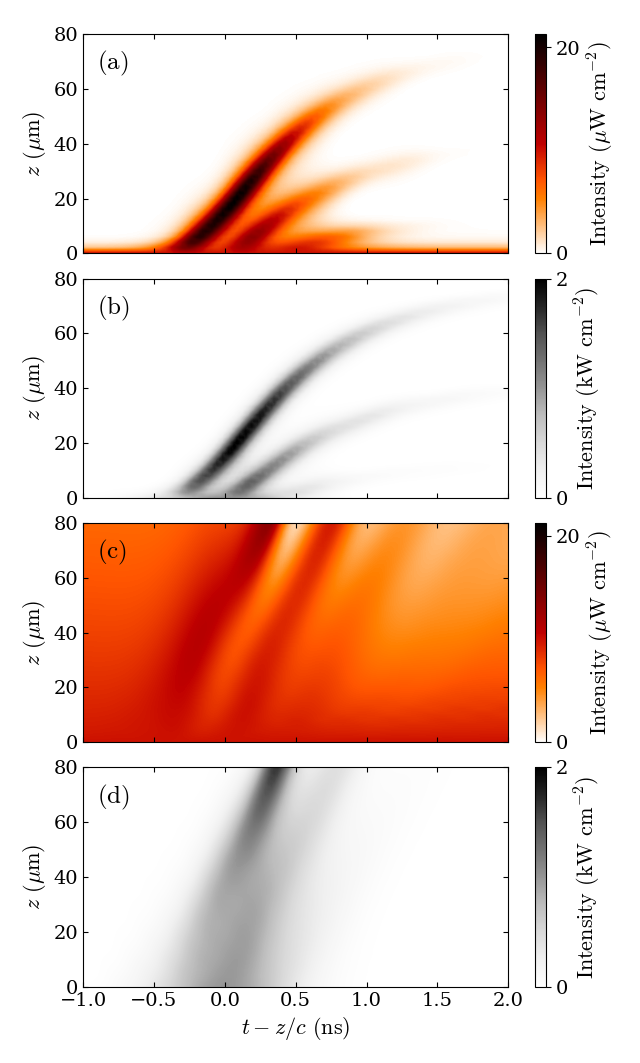
Figure 7: Predictions of the 46-state model including Doppler broadening and self-broadening for two different states of the medium prior to the arrival of the coupling pulse. (a) and (b): the medium is initially in the steady state obtained in the weak field approximation. (c) and (d): the medium is initially in the steady state predicted by the full optical Bloch equations. (a) and (c): the intensity of the probe field. (b) and (d): the intensity of the coupling field.

We generally use the weak field approximation when comparing to the 3-state model, so as to compare like to like. Doing so would not be appropriate when comparing to the data, though, given the strength of the probe field used in the experiment. As the atoms evolve rapidly into a state close if not practically identical to a steady, optically pumped state when they cross the beams, we take the state of the medium prior to the arrival of the coupling pulse to be the exact stationary solution of the optical Bloch equations for the probe field alone. Broadening each state by 30 MHz on account of the interaction with the windows of the nanocell JamesThesis reduces optical pumping, which leads to a larger absorption as would otherwise be the case — compare Figs. S1(c) and (d) to Figs. 5(a) and (b) of the paper.

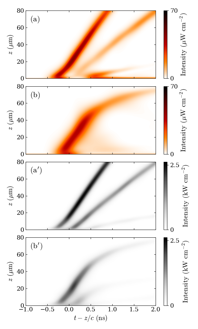
Figure 8: (a) and (a’): the fields obtained within the 46-state model of Fig. 4(b) of the paper. (b) and (b’): the fields obtained when the non-resonant hyperfine levels are ignored. Top two panels: the intensity of the probe field. Bottom two panels: the intensity of the coupling field.

Computations

Like previous investigators old , we worked in terms of the distance $z^{\prime}=z$ and the retarded time $\tau=t-z/c$, in view of the fact that

$${\partial\;\over\partial z}+{1\over c}\,{\partial\;\over\partial t}\rightarrow{\partial\;\over\partial z^{\prime}}$$ (11)

under this change of variables. We divided the relevant ranges of values of $z^{\prime}$ and $\tau$ into a sufficient number of steps — e.g., 16 steps in $z^{\prime}$ in the case of Fig. 2(b) of the paper, but as many as 32,000 in the case of Figs. 3(b) and 3(c). We calculated the fields by integrating the Maxwell-Bloch equations over $z^{\prime}$, starting at $z^{\prime}=0$ (the front of the medium, where the fields have given values): knowing the fields and the polarization of the medium at $z^{\prime}$ (the polarization being calculated as described below), we calculated the fields at $z^{\prime}+\delta z^{\prime}$. We normally used a non-adaptative predictor-corrector approach for this, in which a third-order Adams-Bashforth step was followed by a fourth-order Adams-Moulton step, the fourth-order Runge-Kutta rule being used to start the integration. In some cases, where convergence tests indicated this to be more efficient, we used the second-order Adams-Bashforth rule instead (started with the mid-point formula), without an Adams-Moulton step.

At each step in $z^{\prime}$ we obtained the polarization of the medium by solving the optical Bloch equations. To this effect we used either the fourth-order Runge-Kutta formula or Butcher’s fifth-order Runge-Kutta formula Butcher , whichever was the most efficient for the case at hand. The integral over $v_{z}$ appearing in Eq. (8) was calculated using a 24-point Clenshaw-Curtis rule, which was sufficiently accurate at the temperatures considered.

I Role of the hyperfine structure

Fig. S2 illustrates the importance of taking into account the whole of the hyperfine structure of the levels, not just that of the resonantly coupled 5s${}_{1/2}(F=3)$, 5p${}_{1/2}(F=3)$ and 5p${}_{3/2}(F=4)$ states. Panels (a) and (a’) of this figure show the intensity distribution of the fields inside the medium as calculated with the entire hyperfine structure included (46 states in total), whereas panels (b) and (b’) show the results obtained when only the Zeeman substates of the 5s${}_{1/2}(F=3)$, 5p${}_{1/2}(F=3)$ and 5p${}_{3/2}(F=4)$ states are included. It is clear from Fig. S2 that neglecting the 5s${}_{1/2}(F=2)$, 5p${}_{1/2}(F=2)$ and 5p${}_{3/2}(F=1,2,3)$ states reduces the stability of the quasi-simultons or even prevents their formation. This difference originates from the fact that different pairs of states differing by the values of $m_{F}$ and $m_{F}^{\prime}$ have different transition dipole moments, which compromises the coherent propagation of the two fields through the medium. However, the bandwidth of the coupling pulse ($\sim$ 0.4 GHz for a duration of 0.8 ns) is larger than the hyperfine splitting of the 5p_3/2 level (0.21 GHz) and comparable to that of the 5p_1/2 level (0.36 GHz). The atoms thus tend to couple to the field as if these levels had no hyperfine structure. If the hyperfine splitting was really zero, and ignoring the 5s${}_{1/2}(F=2)$ states (which are far off resonance), the system would be equivalent to the 3-state system discussed in the paper and there would be only a single transition dipole moment for each of the two frequencies. Mathematically, the equivalence arises from the following sum rule,

$$\sum_{F^{\prime}}|\langle 5{\rm s}_{1/2}(F,m_{F}) \,|\,er_{0}\,|\,5{\rm p}_{J^{\prime}}(F^{\prime},m_{F})\rangle|^{2}=$$

$$|\langle 5{\rm s}_{1/2}\,||\,e\,{\bf r}\,||\,5{\rm p}_{J^{\prime}}\rangle|^{2}/3,$$ (12)

which applies for both $F=3$ and $F=2$ and relates the dipole moments of Eq. (9) to those of Eq. (10).

The equivalence with the 3-state model is not exact, though, both because the hyperfine splitting of the 5p states is not completely negligible compared to the bandwidths of the pulse and because only 7/12 of the population is initially in the 5s${}_{1/2}(F=3)$ state in the 46-state model. By contrast, 100% of the population is initially in the ground state in the 3-state model. The density of atoms resonantly coupled to the 5p states by the two fields being smaller in the 46-state model, the quasi-simultons tend to propagate faster in that model than in the 3-state model — e.g., compare Fig. 4(b) of the paper to Fig. 4(a).

By the same token, decreasing the bandwidth of the coupling pulse by increasing its duration also reduces the stability of the quasi-simultons. This is illustrated by Fig. S3. The models, field strengths and coupling pulse duration are the same in panels (a), (a’), (d) and (d’) as in Figs. 4(a) and 4(b) of the paper. Compared to the first column of the figure, the coupling pulse is 2.5 times longer in the second column and 5 times longer in the third column. The peak intensity of this pulse is reduced correspondingly so as to keep its initial area the same (in all three cases, this pulse splits into three solitons in the 3-state model). As seen from the figure, the agreement between the 3-state and 46-state results degrades significantly as the hyperfine splitting of the states starts exceeding the bandwidth of the coupling pulse. For a pulse duration of 4 ns, the probe and coupling fields do no longer co-propagate in the form of clearly defined quasi-simultons.

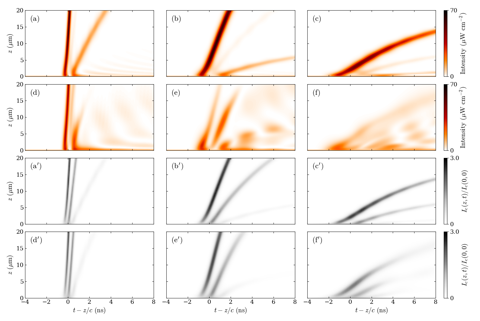
Figure 9: Comparison between the 3-state model of Figs. 3 and 4(a) of the paper and the 46-state model of Fig. 4(b) for different lengths of the coupling pulse. Top two rows: the intensity of the probe field. Bottom two rows: the intensity of the coupling field. (a), (b) and (c), (a’), (b’) and (c’): the 3-state model. (d), (e) and (f), (d’), (e’) and (f’): the 46-state model. (a), (d), (a’) and (d’): $\tau_{\rm c}=0.8$ ns and $I_{\rm c}(z=0,t=0)=1$ kW cm^-2. (b), (e), (b’) and (e’): $\tau_{\rm c}=2$ ns and $I_{\rm c}(z=0,t=0)=0.16$ kW cm^-2. (c), (f), (c’) and (f’): $\tau_{\rm c}=4$ ns and $I_{\rm c}(z=0,t=0)=0.04$ kW cm^-2.

References

- (1) C. P. Pearman, C. S. Adams, S. G. Cox, P. F. Griffin, D. A. Smith and I. G. Hughes, J. Phys. B: At. Mol. Opt. Phys. 35, 5141 (2002).
- (2) J. Keaveney, Ph. D. thesis, Durham University (2013).
- (3) E.g., A. Icsevgi and W. E. Lamb, Jr., Phys. Rev. 185, 517 (1969).
- (4) There are 48 hyperfine 5s and 5p states in total. However, taking the quantization axis parallel to the polarization direction of the coupling field, the 5p states are not coupled to any of the other 46 states.
- (5) D. A. Steck, “Rubidium 85 D Line Data,” available online at http://steck.us/alkalidata (revision 2.1.4, 22 December 2010).
- (6) L. Weller, R. J. Bettles, P. Siddons, C. S. Adams and I. G. Hughes, J. Phys. B: At. Mol. Opt. Phys. 44, 195006 (2011).
- (7) Adding the states to this model and assuming that half the atoms are initially in the ground state and half in the ground state would lead to exactly the same results.
- (8) J. C. Butcher, The Numerical Analysis of Ordinary Differential Equations: Runge-Kutta and General Linear Methods, Wiley, Chichester (1987), Eq. (332e).