New Perspective of Interpretability of Deep Neural Networks
Abstract
Deep neural networks (DNNs) are known as black-box models. In other words, it is difficult to interpret the internal state of the model. Improving the interpretability of DNNs is one of the hot research topics. However, at present, the definition of interpretability for DNNs is vague, and the question of what is a highly explanatory model is still controversial. To address this issue, we provide the definition of the human predictability of the model, as a part of the interpretability of the DNNs. The human predictability proposed in this paper is defined by easiness to predict the change of the inference when perturbating the model of the DNNs. In addition, we introduce one example of high human-predictable DNNs. We discuss that our definition will help to the research of the interpretability of the DNNs considering various types of applications.
Introduction
In recent years, Deep Neural Networks (DNNs) have achieved great success in a number of tasks (?; ?). Nevertheless, the internal state of DNNs are known to be difficult for humans to understand because of their complexity. Due to these black-box properties of the DNNs, numerous iterations of trial-and-error are required to develop the DNN-based applications. One approach to solve this problem is AutoML (?; ?). AutoML is a field of machine learning concerned with automating repetitive tasks such as model selection or hyperparameter optimization. However, AutoML is still a very challenging problem, especially when given complex data.
In practice, human insight is essential to improve the performance of DNN-based applications. This kind of development involving human is called Human-In-The-Loop (HITL) machine learning (?; ?).In the human-in-the-loop approach, people are involved in a virtuous circle where they train, tune, and test a particular algorithm. The goal of HITL machine learning is to train more desired models by human intervention compared to simple end-to-end training. Interpretability and/or explainability of the DNN model is one of the critical aspects of the HITL machine learning.
So-called explainable AI (XAI) has become one of the hot topics in the machine learning field (?; ?). However, a big issue is that the definition of the interpretability and/or explainability of the DNN model is ambiguous.
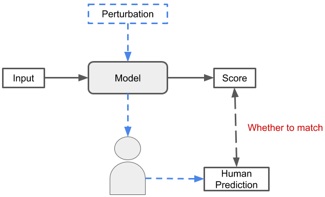
To tackle this problem, we define ”human predictability of the model” as ”easiness for the human to predict the change of the inference when perturbing the model.” Figure 1 shows the overview of our definition. This means that even if the function is complex, the result of the operation on it must match human intuition. In this paper, we show that some functions other than DNNs fit our definition. Furthermore, we propose an example of a neural network architecture and operation pair that satisfies our definition.
Related Works
Humain-In-The-Loop Machine Learning
Human-in-the-loop (HITL) is a research topic of machine learning scheme that leverages both human and machine to create intelligent models. One of the essential paradigms of HITL machine learning is active learning (?). The active learning is a framework that allows humans to select and input training data that maximizes the performance of the next training-step model based on the current model’s output and dataset information. There are several different problem scenarios in active learning.
For example, if we focus on the training data that humans can observe, we can classify them into stream-based and pool-based active learning. In the stream-based active learning (?), humans decide whether to use the training data sampled each time. The stream-based active learning scenario has been studied in several real-world tasks, such as part-of-speech tagging (?) or sensor scheduling (?).
In the pool-based active learning (?), a set of candidate training data is given in advance, and humans select candidate subsets based on the current model output. The pool-based active learning is the major problem setting and has been studied for many tasks, such as image classification (?) and speech recognition (?).
The main difference between the stream-based and the pool-based active learning is that the stream-based active learning obtains the data sequentially and makes query decisions individually, whereas the pool-based active learning evaluates the entire dataset before selecting the best query. In this paper, humans intervene in the context of perturbing to DNNs during inference.
Interpretability of DNNs
Currently, several analyses of the machine learning model’s interpretation have been proposed. We overview some of them.
Sensitivity Analysis
Sensitivity analysis (?; ?) is a method to explain a prediction based on the model’s locally evaluated gradient. Sensitivity analysis quantifies the importance of each input variable as
| (1) |
This measure assumes that the more relevant input features are those to which the output is more sensitive.
Layer-Wise Relevance Propagation
Layer-wise relevance propagation (LRP) (?) explains the classifier’s decisions by decomposition. LRP redistributes the prediction backward via local redistribution rules until it assigns a relevance score to each input variable. Mathematically, the redistribution can be summarized as
| (2) |
The relevance scores define how much the respect variable has contributed to the prediction.
Visual Explanation with Attention Mechanism
There are many studies on visual explanation using attention mechanism (?; ?; ?; ?).
CAM (?) allows us to visualize attention maps for each class using the response of a convolution layer and the weight at the last fully-connected layer. CAM can obtain a good result for weakly-supervised object localization problem but not as well in image classification due to replacing fully-connected layers with convolution layers and passing through global average pooling layer.
Grad-CAM (?) and Grad-CAM++ (?) are the gradient-based visual explanation methods. They can visualize an attention map using positive gradients at a specific class in backpropagation.
Feature Importance
Feature importance approach assumes the importance of a feature by calculating the increase in the model’s prediction error after permuting the feature (?). Permutation feature importance does not require retraining the model or any additional module such as attention mechanism or global average pooling.
Surrogate of Black-Box Model
Surrogate models are trained to approximate the predictions of the underlying black-box model.
LIME (?) focuses on training local surrogate models of the black-box models to explain individual predictions. LIME examine what happens to the predictions when inputting the data into the target model. LIME generates a new dataset consisting of permuted samples and the corresponding predictions of the black-box model. On this new dataset, LIME then trains an interpretable model. The new model is weighted by the proximity of the sampled instances to the instance of interest.
Human Predictability of the Model
The interpretability of the DNNs includes several concepts. The definition of the interpretability of the DDNs is still unclear. In this paper, we introduce the concept of the human predictability of the model, which is closely related to the interpretability. Here, we first provide the definition of the human predictability of the model. Then, we explain it with simple regression models.
Definition
The partial dependence plot and the feature importance are widely used to analyze the relationship between the inference and the input or the feature. Those analyses basically observe the inference while perturbating the input or the feature. The reason why those kinds of numerical analyses are required is that the human cannot predict the tendency of the change of the inference when perturbating the input or the feature. In this sense, if the human can easily predict the tendency of the change of the inference when perturbating the input or the feature of the model, we can say that the model has high interpretability. Based on those observations, in this paper, we define the human predictability of the model by ”easiness to predict the change of the inference when perturbating the model.” In the next subsection, we explain our definition of the human predictability of the model with simple regression models.
Example of Simple Regression Models
Here, we consider simple regression problem for given data , where , with three different regression models: (1) naive polynomials, (2) Legendre polynomials, and (3) Fourier series. The naive polynomial model can be expressed as
| (3) |
where is coefficient. In some senses, the naive polynomial model is straightforward and easy to understand. However, as we discuss later, from the point of view of our definition, the human predictability of the naive polynomial model is not so good, because each term of the naive polynomial is not orthogonal each other.
Legendre polynomials is well-known orthogonal basis, which can be expressed as
| (4) |
where
| (9) | |||||
| (12) |
where is the factorial of . The Legendre polynomial model seems to be complicated compared to the naive polynomial model in Eq. 3. However, it can be considered that the Legendre polynomial model has higher human predictability compared to the naive polynomial model because each term of the Legendre polynomial model is orthogonal each other. That property means that the modification of the coefficient does not affect other terms.
A Fourier series is also known as orthogonal basis, which is expressed as
| (13) |
where and are coefficients.
Now, we compare the human predictability of those three models. Let us consider perturbation for the coefficient of each model. For the Fourier series, the frequency component associated with the perturbed coefficient is only affected. It is straightforward to predict for human. The Legendre polynomial has similar properties to the Fourier series because the Legendre polynomial is the orthogonal basis. The difference between the Legendre polynomial and the Fourier series is the meaning of the basis. The basis of the Legendre polynomial is difficult to imagine for the human, while the base of the Fourier series is easy to imagine for the human because the basis of the Fourier series corresponds the wave with a specific frequency. From those properties, we can say the Fourier series has higher human predictability than the Legendre polynomial. The naive polynomial is the lowest human predictability among the three models because the basis is not orthogonal. It means that the perturbation of the coefficient affects other components. It is difficult to predict the change for human.
Human Predictable DNNs
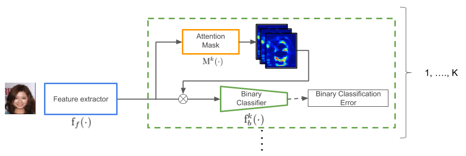
In this section, we introduce one example of human interpretable DNNs which have high human interpretability for the perturbation of the operations of “Semantic Channel Pruning” and “Intentional Attention Mask Transformation.” Figure 2 shows the outline of our proposed network architecture.
Our network basically recognizes multi-attribute for the input image. It is easy to obtain the correlation between features. Our proposed network architecture consists of the following two modules.
-
•
Feature Extractor
-
•
Binary Classifiers with Channel Attention
We aim to obtain highly interpretable neural networks that satisfy our definition using an attention mechanism to acquire features that are important for classifiers.
Feature Extractor
Feature extractor extracts generic feature used by all the following networks. This component performs feature extraction. For this component, we use the dilation network (?). Table 1 shows the detailed architecture of the feature extractor that we used in the experiment.
Binary Classifiers with Attention Mechanism
Binary classifiers , where is number of attributes, are components that perform binary classification corresponding to each attribute of the image. This network is our main component. The loss for the binary classifiers can be expressed by a sum of binary cross entropy of each attribute as
| (15) |
where is the attention mask for -th attribute, and represents element-wise product operation. Note that the attention mask has the same number of channels as that of feature . It differentiates from existing importance visualization algorithms.
The overall loss function is:
| (16) |
where, is the weight parameter, and means sparseness to the attention mask which is used to extract features that are really important for the data. Table 2 shows the detailed architecture of Binary Classifier that we used in the experiment.
Our main idea is to train sub-networks with multi-channel attention mask for each attribute. The attention mask applied to the sub-network is not common in the feature map but has the same number of channels as the feature map. This channel attention mechanism can reveal which channel in the feature map focuses on which part of the image. This transparency of the feature space leads to predictability for perturbing DNNs.
| RGB image |
|---|
| , stride=, padding=, dilation=, conv |
| BatchNorm |
| slope= LeakyReLU |
| , stride=, padding=, dilation=, conv |
| BatchNorm |
| slope= LeakyReLU |
| , stride=, padding=, dilation=, conv |
| BatchNorm |
| slope= LeakyReLU |
| , stride=, padding=, dilation=, conv |
| BatchNorm |
| slope= LeakyReLU |
| Attention Mask |
| Global Average Pooling |
| sigmoid |
Semantic Channel Pruning
In this section, we introduce Semantic Channel Pruning as an example of an operation for a human-predictable neural network. Channel pruning (?; ?) is a technique for acquiring sparse DNNs by removing channels in the layers. Identifying the informative (or important) channels, also known as channel selection, is a key issue in channel pruning. Therefore, we present an example of channel selection using our proposed human-predictable network architecture.
Figure 3 shows the overview of Semantic Channel Pruning operation. Our main idea is that we do not need multiple channels for a specific role. In other words, we assume that if there are multiple channels with similar roles, it is possible to prune all but one.
First, we train the network with the proposed architecture. Next, we use the trained network and the training data to calculate the correlation matrix among the channels of the network. Note that the weight of the trained network is fixed at this time. Finally, we sequentially scan the highly correlated channel pairs and prune the channel with the lower -norm of the weights. Our proposed network architecture that accepts this operation satisfies our definition.
| Method | Average of accuracy [%] |
|---|---|
| FaceTracer | 81.13 |
| PANDA-1 | 85.43 |
| LNet+ANet | 87.30 |
| MOON | 90.93 |
| ABN | 91.07 |
| ResNet101 | 90.69 |
| Ours | 90.72 |
Intentional Attention Mask Transformation
Here, we propose the ”Intentional Attention Mask Transformation” to improve the robustness of CNNs. Our main idea is to reduce the effect of noise by only focusing on important features area for the classification of each attribute. To achieve this goal, we introduce the following simple attention mask transformation function .
| (17) | |||||
| (18) |
where and are parameters to adjust the emphasis and suppression of the mask. The function is symmetric with respect to 0.5, and the function emphasizes large values in the mask .
The output of a binary classifier applying our intentional attention mask transformation is:
| (19) |
The above equations emphasize important features about the attribute of sample .
This transformation function is similar to the intensity tone curve in image retouching. In this paper, the symmetric function inspired by the tone curve is used as the transformation function, and the slope and bias of the symmetric function are used as the side information, but any function and side information (such as prior knowledge of data) can be used.
According to our definition, a model that accepts this operation can be said to be human-predictable because we can know in advance the accuracy change when we change internal parameters.
| Target Attribute | Top5 Highly Correlated Attributes |
|---|---|
| Black Hair | Blond Hair, Brown Hair, Bald, Wearing Hat, Gray Hair |
| Heavy Makeup | Wearing Lipstick, Male, Rosy Cheeks, Attractive, Young |
| Bushy Eyebrows | Bags Under Eyes, Eyeglasses, Arched Eyebrows, Heavy Makeup, Attractive |
Experimental Results
We evaluate our approach using the CelebA dataset (?), which consists of 40 facial attribute labels and 202,599 images (182,637 training images and 19,962 testing images). The parameter of sparseness in Eq. 16 is . The dimension of the attention mask and feature map is 128. Tables 1 and 2 show the details of the network architecture used in this experiment.
Table 3 shows the overall test accuracies of several networks. We evaluate the accuracy rate using FaceTracer (?), PANDA (?), LNet+ANet (?), mixed objective optimization network (MOON) (?), Attention Branch Network (ABN) (?) and ResNet101. Although the accuracy of our network is not the best, our aim is to increase the interpretability of the network. In this sense, the performance of the proposed network is reasonably good, even compared with the state-of-the-art network.
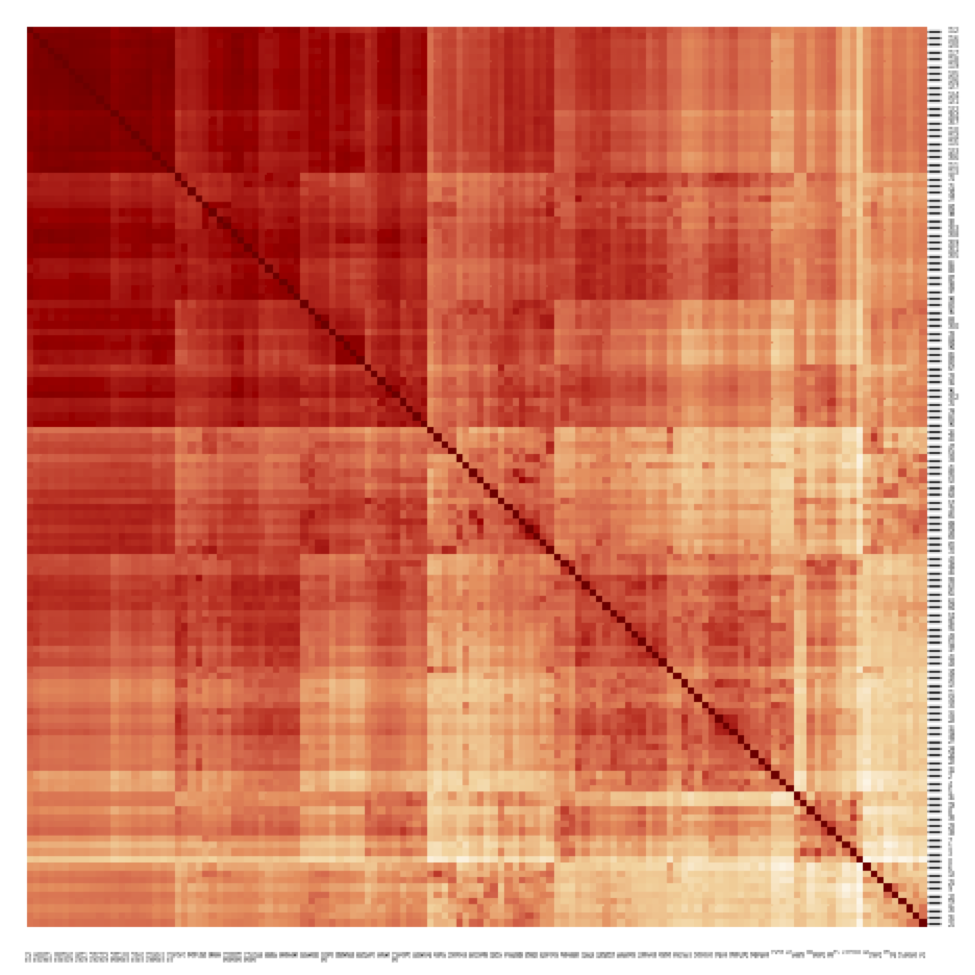
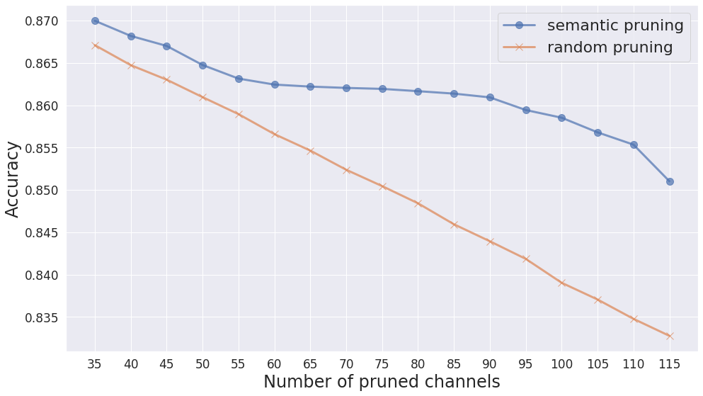
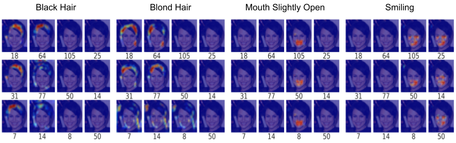
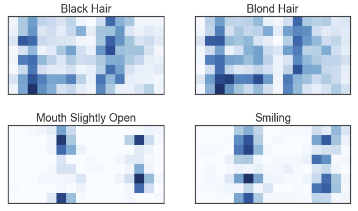
Figure 4 shows the visualization of the attention mask by our proposed method. In this figure, common feature channels are visualized for each attribute, and each column means the top three features which have high importance for each attribute. Our attention masks focus on areas that may be important to attributes. In addition, this experimental result suggests that analysis of feature space reveals the relationship among attributes. For example, feature IDs 25, 14 and 50 are not used to predict the attribute of Mouse Slightly Open, although they are used for the attribute of Smiling. On the other hand, IDs 105 and 50 are commonly used in the attributes of Smiling and Mouse Slightly Open, and ID 8 is not used in Smiling. Only the mouth region is focused for the attribute of Mouse Slightly Open, while a broad part including mouse and eyes are focused for the attribute of Smiling. Those results are consistent with human intuition. In addition, it can be seen that even in different channels, there are cases where attention focus to the same location in the image.
The network architecture we proposed in the previous section can reveal channels that are similar in the role. Figure 6 shows the visualization of the correlations between features.
Figure 5 shows a grid visualization of the mean values of each channel of attention masks. Our analysis reveals that similar channels of features are commonly used for attributes of ”Black Hair” and ”Blond Hair.” Relevant channels for attributes of ”Mouth Slightly Open” and ”Smiling” are also similar.
Table 4 lists some of the attributes and their highly correlated attributes. Here, we calculate the correlation among attention masks corresponding to each attribute. In other words, considering the data in Figure 5 as one vector data, Table 4 uses the correlation of the vector data. Attributes that are intuitively similar are highly correlated. This result makes it possible to group highly correlated attributes. In addition, experimental results may even reveal potential relationships among attributes. In other words, our network architecture makes it easy for humans to understand changes in the internal structure of the network.
Channel Pruning Experiment
Previous results allow us to prune unnecessary channels after understanding the role of each channel in the network. In our proposed method, the group of channels with the same role becomes the target of pruning. The channel to be pruned is determined based on the correlation matrix in Figure 6, that is, the channel pair with high correlation in the correlation matrix is considered as a pair with similar roles, and the channel with the higher -norm is pruned.
Figure 7 shows the experimental result of our Semantic Channel Pruning operation. We gradually increased the number of channels to be pruned and evaluated the transition of classification performance. In random pruning, the performance degrades linearly as the number of pruned channels increases. On the other hand, we can see that our proposed channel pruning method selects meaningful channels compared to random selection.
Mask Transformation Experiment
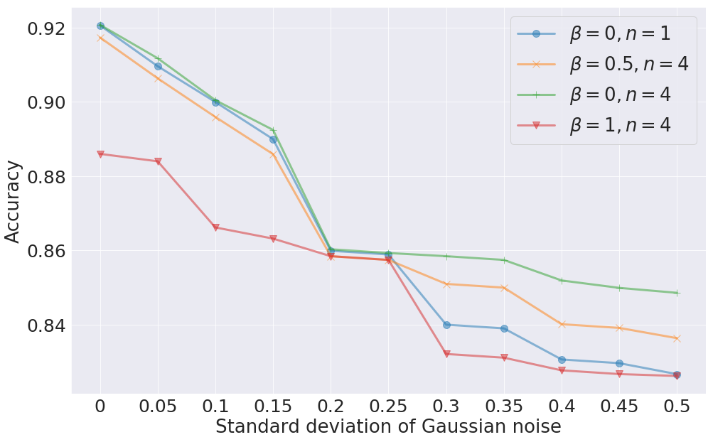
We evaluate the robustness of the network by the Intentional Attention Mask Transformation. We add Gaussian noise with a standard deviation of 0 to 0.5 to the input images to create pseudo noisy data. Figure 8 shows the experimental results of observing the transition of the performance for this noisy input data for a combination of multiple parameters. The experimental results show that the transformation of the attention mask makes the network robust against performance degradation due to noise. The result of and is the performance transition of the network without the intentional attention mask transformation, and by adjusting and , the performance improvement for noisy input is achieved.
Conclusion
In this paper, We proposed the novel aspect of the interpretability of DNNs. We define ”human predictability of the model” as ”easiness for the human to predict the change of the inference when perturbing the model.” This means that even if the function is complex, the result of the operation on it must match human intuition. Furthermore, we propose an example of a neural network architecture and operation pair that satisfies our definition.
We suggest that considering various applications according to our definition will lead to a wide range of research. As one of the future works, we need to find more model-operation pairs that satisfy our definition and show the potential for the broader application of our definition.
References
- [Bach et al. 2015] Bach, S.; Binder, A.; Montavon, G.; Klauschen, F.; Müller, K.-R.; and Samek, W. 2015. On pixel-wise explanations for non-linear classifier decisions by layer-wise relevance propagation. PloS one 10(7):e0130140.
- [Baehrens et al. 2010] Baehrens, D.; Schroeter, T.; Harmeling, S.; Kawanabe, M.; Hansen, K.; and MÞller, K.-R. 2010. How to explain individual classification decisions. Journal of Machine Learning Research 11(Jun):1803–1831.
- [Chattopadhay et al. 2018] Chattopadhay, A.; Sarkar, A.; Howlader, P.; and Balasubramanian, V. N. 2018. Grad-cam++: Generalized gradient-based visual explanations for deep convolutional networks. In 2018 IEEE Winter Conference on Applications of Computer Vision (WACV), 839–847. IEEE.
- [Dagan and Engelson 1995] Dagan, I., and Engelson, S. P. 1995. Committee-based sampling for training probabilistic classifiers. In Machine Learning Proceedings 1995. Elsevier. 150–157.
- [Dasgupta, Hsu, and Monteleoni 2008] Dasgupta, S.; Hsu, D. J.; and Monteleoni, C. 2008. A general agnostic active learning algorithm. In Advances in neural information processing systems, 353–360.
- [Deng et al. 2009] Deng, J.; Dong, W.; Socher, R.; Li, L.-J.; Li, K.; and Fei-Fei, L. 2009. Imagenet: A large-scale hierarchical image database. In 2009 IEEE conference on computer vision and pattern recognition, 248–255. Ieee.
- [Elsken, Metzen, and Hutter 2018] Elsken, T.; Metzen, J. H.; and Hutter, F. 2018. Neural architecture search: A survey. arXiv preprint arXiv:1808.05377.
- [Fails and Olsen Jr 2003] Fails, J. A., and Olsen Jr, D. R. 2003. Interactive machine learning. In Proceedings of the 8th international conference on Intelligent user interfaces, 39–45. ACM.
- [Fisher, Rudin, and Dominici 2018] Fisher, A.; Rudin, C.; and Dominici, F. 2018. Model class reliance: Variable importance measures for any machine learning model class, from the “rashomon” perspective. arXiv preprint arXiv:1801.01489.
- [Fukui et al. 2019] Fukui, H.; Hirakawa, T.; Yamashita, T.; and Fujiyoshi, H. 2019. Attention branch network: Learning of attention mechanism for visual explanation. In Proceedings of the IEEE Conference on Computer Vision and Pattern Recognition, 10705–10714.
- [Gunning 2017] Gunning, D. 2017. Explainable artificial intelligence (xai). Defense Advanced Research Projects Agency (DARPA), nd Web 2.
- [He, Zhang, and Sun 2017] He, Y.; Zhang, X.; and Sun, J. 2017. Channel pruning for accelerating very deep neural networks. In Proceedings of the IEEE International Conference on Computer Vision, 1389–1397.
- [Holzinger 2016] Holzinger, A. 2016. Interactive machine learning for health informatics: when do we need the human-in-the-loop? Brain Informatics 3(2):119–131.
- [Kimura and Tanaka 2019] Kimura, M., and Tanaka, M. 2019. Interpretation of feature space using multi-channel attentional sub-networks. In Proceedings of the IEEE Conference on Computer Vision and Pattern Recognition Workshops, 36–39.
- [Krishnamurthy 2002] Krishnamurthy, V. 2002. Algorithms for optimal scheduling and management of hidden markov model sensors. IEEE Transactions on Signal Processing 50(6):1382–1397.
- [Kumar, Belhumeur, and Nayar 2008] Kumar, N.; Belhumeur, P.; and Nayar, S. 2008. Facetracer: A search engine for large collections of images with faces. In European conference on computer vision, 340–353. Springer.
- [Lewis and Catlett 1994] Lewis, D. D., and Catlett, J. 1994. Heterogeneous uncertainty sampling for supervised learning. In Machine learning proceedings 1994. Elsevier. 148–156.
- [Liu et al. 2015] Liu, Z.; Luo, P.; Wang, X.; and Tang, X. 2015. Deep learning face attributes in the wild. In Proceedings of the IEEE international conference on computer vision, 3730–3738.
- [Liu et al. 2017] Liu, W.; Wang, Z.; Liu, X.; Zeng, N.; Liu, Y.; and Alsaadi, F. E. 2017. A survey of deep neural network architectures and their applications. Neurocomputing 234:11–26.
- [Ribeiro, Singh, and Guestrin 2016] Ribeiro, M. T.; Singh, S.; and Guestrin, C. 2016. Why should i trust you?: Explaining the predictions of any classifier. In Proceedings of the 22nd ACM SIGKDD international conference on knowledge discovery and data mining, 1135–1144. ACM.
- [Rudd, Günther, and Boult 2016] Rudd, E. M.; Günther, M.; and Boult, T. E. 2016. Moon: A mixed objective optimization network for the recognition of facial attributes. In European Conference on Computer Vision, 19–35. Springer.
- [Samek, Wiegand, and Müller 2017] Samek, W.; Wiegand, T.; and Müller, K.-R. 2017. Explainable artificial intelligence: Understanding, visualizing and interpreting deep learning models. arXiv preprint arXiv:1708.08296.
- [Settles 2009] Settles, B. 2009. Active learning literature survey. Technical report, University of Wisconsin-Madison Department of Computer Sciences.
- [Simonyan, Vedaldi, and Zisserman 2013] Simonyan, K.; Vedaldi, A.; and Zisserman, A. 2013. Deep inside convolutional networks: Visualising image classification models and saliency maps. arXiv preprint arXiv:1312.6034.
- [Tong and Chang 2001] Tong, S., and Chang, E. 2001. Support vector machine active learning for image retrieval. In Proceedings of the ninth ACM international conference on Multimedia, 107–118. ACM.
- [Tur, Hakkani-Tür, and Schapire 2005] Tur, G.; Hakkani-Tür, D.; and Schapire, R. E. 2005. Combining active and semi-supervised learning for spoken language understanding. Speech Communication 45(2):171–186.
- [Ye et al. 2018] Ye, J.; Lu, X.; Lin, Z.; and Wang, J. Z. 2018. Rethinking the smaller-norm-less-informative assumption in channel pruning of convolution layers. arXiv preprint arXiv:1802.00124.
- [Yu and Koltun 2016] Yu, F., and Koltun, V. 2016. Multi-scale context aggregation by dilated convolutions. In International Conference on Learning Representations.
- [Zhang et al. 2014] Zhang, N.; Paluri, M.; Ranzato, M.; Darrell, T.; and Bourdev, L. 2014. Panda: Pose aligned networks for deep attribute modeling. In Proceedings of the IEEE conference on computer vision and pattern recognition, 1637–1644.
- [Zhou et al. 2016] Zhou, B.; Khosla, A.; Lapedriza, A.; Oliva, A.; and Torralba, A. 2016. Learning deep features for discriminative localization. In Proceedings of the IEEE conference on computer vision and pattern recognition, 2921–2929.
- [Zoph and Le 2016] Zoph, B., and Le, Q. V. 2016. Neural architecture search with reinforcement learning. arXiv preprint arXiv:1611.01578.