Quantum phase communication channels assisted by non-deterministic noiseless amplifiers

Abstract

We address quantum $M$-ary phase-shift keyed (PSK) communication channels in the presence of phase diffusion, and analyze the use of probabilistic noiseless linear amplifiers (NLA) to enhance performance of coherent signals. We consider both static and dynamical phase diffusion and assess the performances of the channel for ideal and realistic phase receivers. Our results show that NLA employed at the stage of signal preparations is a useful resource, especially in the regime of weak signals. We also discuss the interplay between the use of NLA, and the memory effects occurring with dynamical noise, in determining the capacity of the channel.

1 Introduction

Quantum communication channels based on continuous variables (CV) have attracted an increasing interest in the recent years, due to their robustness against noise [1]. For lossless CV channels, the capacity at fixed energy is maximised by thermal encoding of information onto Fock states[2]. On the other hand, when propagation and detection are affected by loss and/or noise, alternative strategies, where information is encoded onto either the phase or the amplitude of coherent signals, have proven effective [3, 4].

In a phase modulation scheme, where the information is encoded in the phase of a quantum seed signal [5, 6], the most detrimental noise is phase diffusion [7, 8]. In particular, when the seed state is coherent, it has been shown that time-independent Markovian noise is detrimental to information transfer and may undermine the overall performance of the channel [9, 10]. However, in quantum optical communications, the Markovian hypothesis may be violated by the spectral structure of the environment leading to non-Markovian damping or diffusion channels [10, 11]. Thereby, reservoir engineering may lead to substantial improvements in optical communication channels, by properly handling the unavoidable interaction with the environment during propagation.

More generally, in order to reduce the detrimental effects of the noise, and the corresponding loss of information, different types of amplification processes may be employed. None of them, however, is expected to restore ideal conditions, due to the inherent quantum limits of amplification. In particular, the noise figure $R$ (i.e. the ratio between the input and the output, signal-to-noise ratios) of linear quantum amplifiers is bounded by $R>2$, leading to the well known $3$dB standard quantum noise limit [12]. In this paper, we exploit the possibility of overcoming a possible this fundamental quantum limitation is by means of probabilistic amplification based on conditional dynamics in quantum phase communication channels. Furthermore, we investigate the use of probabilistic (and noiseless) linear amplifier (NLA) at the stage of signal preparation to improve the performances of noisy phase channels based on coherent signals.

We consider a protocol where information is encoded in the phase-shift of a seed state, which is then transferred to a receiver station along a transmission line where phase diffusion (static noise) or phase fluctuations (dynamical noise) may occur. We consider static phase noise induced by a Markovian environment as well as a dynamical noise leading to non-Markovian evolution. We evaluate the mutual information for NL-amplified coherent states for both ideal and realistic phase receivers at the detection stage. In practice, the successfully (heralded) amplified states serve as careers for phase information transmission processes, and undergo the whole process of encoding-transfer along the noisy channel-decoding, whereas when the amplification fails, the sender abstains from imprinting letters in the distorted states and discard them instead. We then compare their performances and also compare those phase channels to noisy amplitude-based ones, where information is encoded onto the amplitude of coherent states. Finally, we discuss the interplay between the use of NLA and the memory effects occurring with dynamical noise in determining the capacity of the channel.

Among the different possible implementations of NLA schemes, we focus attention on a feasible one [13] which, in turn, has been experimentally achieved with current technology [14], at least for a given values of the gain. Our results are therefore of practical interest and may be experimentally verified.

The paper is organized as follows. In sec 2, we review the model of the probabilistic linear amplifier considered in our work and address its action on coherent states. In section 3, we describe in some details of the dephasing dynamics. We then review, in sec 4 the main steps of the encoding-decoding strategy in the quantum phase channel. Sec 5 is devoted to illustrate our results for both static and dynamical phase noise. Finally, sec 6 closes the paper with some concluding remarks.

2 Model of the noiseless linear amplifier

An ideal, noiseless deterministic amplification of a quantum state is inherently forbidden by the unitarity and linearity of quantum evolution. In fact, so as to reinstate the uncertainty principle, an unavoidable noise has to be introduced. A quantum-noise limit has been drawn up for both the two versions of linear deterministic amplifiers: phase-sensitive and phase-insensitive [12]. Recently, much attention has been devoted to a new generation of linear amplifiers whose action differs from the conventional devices: probabilistic noiseless amplifiers [15]. In turn, the non-deterministic nature of those devices enables to elude the theoretical limitation prohibiting noiseless amplification. Hereafter, several theoretical schemes and implementation of the NLA have been proposed [16, 17, 18, 19]. Here, we consider the theoretical model suggested in [13] and experimentally demonstrated in [14] for a given value of the gain.

Let us now describe the noiseless amplification in the Schrödinger picture, where it may be perceived as the operation that takes a coherent state $|\alpha\rangle$ to its approximated amplified version $|g\alpha\rangle$ with a rate of success $p_{s}$ that depends on the mean energy of the input state. A probabilistic noiseless amplification may thus be described by the non-unitary operator

$${\mathcal{M}}(g)=g^{{a^{\dagger}a}}\,,$$ (1)

$a$ being the field mode operator. The instance we are interested is $g>1$, where $g$ refers to the gain of the amplifier. The action of such operator on Fock states $|n\rangle$ consists to assign a factor $g^{n}$ to their amplitudes. The operator ${\mathcal{M}}(g)$ is unbounded, and the physical consequence of this mathematical issue is that a noiseless amplification may only be approximately achieved with a finite success probability. In particular, it may be implemented by truncating the expansion of $g^{{a^{\dagger}a}}$ to a given order in the number operator, that we refer to as the truncation order. This approximation is well justified for the class of weak signals we are going to consider in the following. In particular, let us consider the case where the truncation order is set to one. A good figure of merit to assess the performance of the amplification process is the so-called effective gain, defined as the ratio of the amplitude of the amplified state

$${\varrho}_{\text{a}}=\frac{\mathcal{M}(g)|\alpha\rangle\langle\alpha|\mathcal{M}^{\dagger}(g)}{\operatorname{tr}\left[\mathcal{M}(g)|\alpha\rangle\langle\alpha|\mathcal{M}^{\dagger}(g)\right]}\,,$$

to that of the input coherent state, i.e.

$$g_{\text{eff}}=\frac{1}{\alpha}\operatorname{tr}\left[{a}\,{\varrho}_{\text{a}}\right].$$ (2)

Fundamental constraints to noiseless amplification require the fidelity of the output state to the ideally amplified coherent state to approach unit value and the effective and nominal gains to coincide $g_{\text{eff}}=g$ in the limit of vanishing input energies. Upon truncating the Taylor series expansion of the NLA operator in its first order and fulfilling the previously raised constraints, we derive the expression of the approximate NLA operator [14]

$$\mathcal{M}(g)=1+\left(g-1\right){a^{\dagger}a}.$$ (3)

In the following, we refer to the state resulting from the action of the approximate NLA in Eq. (3) on coherent input as (AC) $|\alpha\rangle_{\text{a}}$. Its density matrix elements in the Fock basis may be expressed as follows

$$\varrho_{n,m}=\frac{e^{-\bar{n}}}{\mathcal{A}}\frac{\bar{n}^{\frac{n+m}{2}}}{\sqrt{n!\,m!}}\big{[}1+(g-1)n\big{]}\big{[}1+(g-1)m\big{]}\,,$$ (4)

where $\bar{n}$ denotes the average photons number and $\mathcal{A}^{-1}$ a normalisation constant given by

$$\mathcal{A}=1+\left(g^{2}-1\right)\bar{n}+\left(g-1\right)^{2}\bar{n}^{2}\,,$$ (5)

As it is apparent from Eq. (3), the NLA with gain $g=2$ reduces to photon addition and photon subtraction [20] performed in a sequence, a procedure which is experimentally available [14] with current technology. It is worth noting that the model of NLA considered throughout the paper presents several advantages compared to other physical schemes, as demonstrated by its performances quantified by the effective gain and fidelity [14]. Besides the realistic implementations mentioned so far, more abstract schemes for noiseless amplification have been recently proposed [21, 22, 23]. Their operating principle is based on a postselection of classical data collected from heterodyne detection that emulate a noiseless amplification. Despite being experimentally friendly, as only feasible Gaussian operations are required, the emulated NLA is not suited for our protocol due to the restrictive need of being directly followed by a heterodyne detection, thereby embedded within the detection stage.

3 Static and dynamical phase diffusion

This section is devoted to model the dynamics induced by a phase diffusive classical environment on a continuous variable system. In particular, we show that treating the environment as a classical stochastic field (CSF) provides an effective description of the dynamics, able to describe rich phenomenology that canonical Master Equations approach, usually derived from too restrictive approximations, may not capture.

Let us consider a single bosonic mode interacting with a classical stochastic field (CSF). The dynamics of the system is governed by the total Hamiltonian, i.e. the sum of the free and interaction Hamiltonians given respectively by

$${H}_{0}=\hbar\omega_{0}{a}^{\dagger}{a}$$ (6)

$${H}_{i}=\hbar{a}^{\dagger}{a}\left[F(t)e^{-i\omega t}+F^{*}(t)e^{i\omega t}\right]$$ (7)

where $\omega_{0}$ is the proper frequency of the oscillator and $F(t)e^{-i\omega}$ an external fluctuating field with a complex amplitude that oscillates in time with a central frequency $\omega$. $F(t)$ describes the realizations of a stochastic process with zero mean, accounting for the noise induced by the surrounding degrees of freedom and $F(t)^{*}$ denotes its complex conjugate. As the interaction and free Hamiltonians commute, the Hamiltonian operator in the interaction picture reads (in units of $\hbar$)

$${H}={a}^{\dagger}{a}\left[F(t)e^{-i\omega t}+F^{*}(t)e^{i\omega t}\right]$$ (8)

where the stochastic field $F(t)$ assume a dimension of frequency. The Hamiltonian being self-commuting at different times, i.e. $\left[{H}(t),{H}(t^{{}^{\prime}})\right]=0$, the evaluation of the evolution operator expression is made straightforward. As it appears, the evolution operator coincides with a unitary phase-shift :

$${U}(t)=e^{i\phi(t){a}^{\dagger}{a}}$$ (9)

where $\phi(t)=\int_{0}^{t}ds\left[F(s)e^{-i\omega s}+F(s)^{*}e^{i\omega s}\right]$ accounts for the phase-shift performed on the system and depends essentially on the (CSF). After expanding the initial state in a Fock basis, the evolved density matrix at time $t$ reads

$${\varrho}(t)= \left\langle{U}(t){\varrho}(0){U}^{\dagger}(t)\right\rangle_{F}$$ (10)

$$= \sum_{n,m}\left\langle e^{-i\phi(t)(n-m)}\right\rangle_{F}\varrho_{nm}|n\rangle\langle m|,$$

where $\left\langle.\right\rangle_{F}$ represents the average over all possible realisations of the stochastic process. From now on, we consider Gaussian stochastic processes that are fully characterized by their two first order statistics, that is, the mean $\mu(t)=\left\langle F(t)\right\rangle_{F}$ and the autocorrelation function $K(t,t^{{}^{\prime}})=\left\langle F(t)F(t^{\prime})\right\rangle_{F}$. In particular, we will focus on stochastic fields with zero mean and autocorrelation matrix assuming a diagonal form

$$\left\langle\mathcal{R}\left[F(t)\right]\mathcal{R}\left[F(t^{\prime})\right]\right\rangle_{F}=\left\langle\mathcal{I}\left[F(t)\right]\mathcal{I}\left[F(t^{\prime})\right]\right\rangle_{F}=K(t,t^{{}^{\prime}})$$ (11)

$$\left\langle\mathcal{R}\left[F(t)\right]\mathcal{I}\left[F(t^{\prime})\right]\right\rangle_{F}=\left\langle\mathcal{I}\left[F(t)\right]\mathcal{R}\left[F(t^{\prime})\right]\right\rangle_{F}=0,$$ (12)

where $\mathcal{R}\left[F(t)\right]$ and $\mathcal{I}\left[F(t)\right]$ denote respectively the real and the imaginary parts of the stochastic field. The rearrangement of the phase $\phi(t)$ in terms of two distinct contributions coming from the real and imaginary parts of the (CSF) simplifies remarkably the evaluation of the evolved density matrix. The average in Eq (10) reduces to the evaluation of the joint characteristic function of two Gaussian variables

$$\left\langle e^{-i\phi(t)(n-m)}\right\rangle_{F}=e^{-\frac{1}{2}(n-m)^{2}\sigma(t)},$$ (13)

with $\sigma(t)$ being a function that depends on the kernel of the stochastic process

$$\sigma(t)=\int_{0}^{t}\int_{0}^{t}dsds^{\prime}cos\left[\omega(s-s^{\prime})\right]K(s,s^{\prime}).$$ (14)

The evolved density matrix of Eq (10) then simplifies to

$${\varrho}(t)=\sum_{n,m}e^{-\frac{1}{2}(n-m)^{2}\sigma(t)}\varrho_{n,m}|n\rangle\langle m|.$$ (15)

As it appears the diagonal elements $\varrho_{nn}$ are left unchanged under the phase diffusion, thus preserving the occupation probabilities, while the off-diagonal matrix elements vanish exponentially. When $\sigma(t)$ displays a linear behaviour in time, the Gaussian process is said to be static. In that case, one recovers the solution of the Master Equation that governs the evolution of a system undergoing Markovian phase diffusion noise. We defer a detailed discussion for the following parts where a specific model of Gaussian stochastic process (the power-law process) will be analyzed.

4 Quantum phase-shift keyed communication

In phase-modulation-based communication channels $M$ symbols selected from a given ensemble are encoded using $M$ uniformly spaced phase shifts $\phi_{l}$ ranging from $0$ to $2\pi$. The encoding procedure is carried out by a phase-shift operation ${U}(\phi_{l})$ on a seed single-mode state ${\varrho}_{0}$ that yields the deterministic state ${\varrho}_{l}={U}(\phi_{l}){\varrho}_{0}{U}^{\dagger}(\phi_{l})$. Next, the signal ${\varrho}_{l}$ is sent through a transmission line to a receiving station where a phase measurement, followed by a suitable inference strategy are performed so as to extract the information. A straightforward strategy consists on dividing the ensemble of possible outcomes to $M$ intervals

$$\Sigma_{l}=\left[\phi_{l}-\frac{\Delta}{2},\phi_{m}+\frac{\Delta}{2}\right)\,,$$

of width $\Delta=2\pi/M$ and associate each measured phase that falls into $\Sigma_{l}$ with the corresponding symbol that the phase-shift $\phi_{l}$ accounts for. It’s evident that the intervals $\Sigma_{l}$ sum up to $\left[0,2\pi\right)$. We point out that, naturally, one may opt for a different inference strategy where a non-uniform width of the intervals is chosen. As a symmetric choice is generally optimal, we adopt the previously-presented scheme that may be summarized in the following terms: for each outcome $\phi$ of the phase measurement, if $\phi\in\Sigma_{l}$, then $\phi\mapsto\phi_{l}$. The statistics of a phase measurement outcomes are described by a positive operator-valued measure (POVM) $\left\{\pi(\theta)\right\}$ where $\theta\in\left[0,2\pi\right)$. The recipe that provides the probabilities of the receiver’s outcomes $\Pi_{l}$ reads as [24]

$${\Pi}_{l}=\int_{\Sigma_{l}}\pi(\theta)d\theta.$$ (16)

A covariant phase measurement can always be described by a POVM $\left\{\pi(\theta)\right\}$ that assumes the following form:

$${\pi}(\theta)=\frac{1}{2\pi}\sum_{n,m=0}^{\infty}\,A_{n,m}\,e^{-i(n-m)\theta}|n\rangle\langle m|,$$ (17)

where $A_{n,m}=2\pi\langle m|{\pi}(0)|n\rangle$ are the elements of a positive and Hermitian matrix $A$ set by the chosen phase measurement. We remark that the covariance of the phase measurement performed by the receiver is ensured by the covariance property of $\left\{{\pi}(\theta)\right\}$. This implies :

$${\Pi}_{l}(\theta)={U}(\phi_{l}){\Pi}(0){U}^{\dagger}(\phi_{l}).$$ (18)

Starting from Eqs (17) and (16), we arrive to the compact formula

$${\Pi}_{l}(\theta)=\sum_{n,m=0}^{\infty}A_{n,m}f_{n-m}(l)|n\rangle\langle m|$$ (19)

where $f_{d}(l)=\frac{1}{2\pi}\int_{\Sigma_{l}}e^{-id\theta}d\theta$ refers to as the resolution function. Since the phase-shifts are equidistant ($\phi_{l}=2\pi l/M$) and the range of possible outcomes is uniform, the resolution function assumes the following form

$$f_{d}(l)=\frac{e^{-\frac{2\pi ld}{M}}}{\pi d}\sin{\frac{\pi d}{M}}.$$ (20)

In order to quantify the performance of the phase-shift keyed communication channel, we employ the mutual information (MI) between output and input, as a suitable figure of merit that measures the amount of information transferred along the transmission line at each use of the channel. MI is given by: $I=S(O)-S(O|I)$, $S(O)=\sum_{l=0}^{M-1}p^{\prime}(l)\log{\left(p^{\prime}(l)\right)}$ being the total information available at the receiver (output) and $S(O|I)=\sum_{k=0}^{M-1}p(k)S(O|k)=\sum_{l,k=0}^{M-1}p(k)p(l|k)\log{p(l|k)}$ the conditional information available at the output knowing which element ($\phi_{k}$) from the input ensemble was sent averaged over the possible inputs. We clearly notice that the mutual information is determined by three quantities: the prior probability that a given symbol ($\phi_{k}$) carried by the state ${\varrho}_{k}$ was transmitted, the probability for the receiver to read out a given symbol ($\phi_{l}$), that reads $p^{\prime}(l)=\sum_{k=0}^{M-1}p(l|k)p(k)$ and finally, the conditional probability $p(l|k)$ for the receiver to measure a phase ($\phi_{l}$) given that the input symbol encoded in ($\phi_{k}$) was transmitted. The classical channel capacity, namely the maximum information reliably transferred through the transmission line per use is given by the maximum over the prior probability $p(k)$ of the mutual information. Throughout this paper, we assume a uniform prior. In other words, the states ${\varrho}_{k}$ are transmitted according to the same probability i.e. ($p(\phi_{k})\equiv p(k)=1/M$). Hence, the evaluation of the mutual information depends mainly on the conditional probability $p(j|k)$ and its expression reads

$$I=\frac{1}{M}\sum_{l,k=0}^{M-1}p(l|k)\log{\frac{Mp(l|k)}{\sum_{k=0}^{M-1}p(l|k)}}.$$ (21)

The conditional probability $p(l|k)$ is thought as the probability that a measurement outcome belongs to the phase interval $\Sigma_{l}$ when the state ${\varrho}_{k}$ has been actually transmitted along the channel. Owing to the covariance property of the POVM ${{\Pi}_{l}}$, its expression can be written as

$$p(l|k)= \operatorname{tr}{\left[{\varrho}_{k}{\Pi}_{l}\right]}=\operatorname{tr}{\left[{\varrho}_{0}{\Pi}_{l-k}\right]}$$ (22)

$$= \sum_{n,m=0}^{\infty}A_{n,m}f_{n-m}(l-k)\varrho_{n,m}.$$

Besides, making use of the symmetries of the resolution function $f_{-d}(-l)=f_{d}(l)$, and upon introducing the positive index $s=\left|l-k\right|$ ranging from 0 to $M-1$, the mutual information (21) simplifies to

$$I\equiv I(M,\bar{n})=\log{M}+\sum_{s=0}^{M-1}q(s)\log{q(s)},$$ (23)

with $\bar{n}$ being the average photons number of the input state and $q(s)=\sum_{n,m=0}^{\infty}A_{n,m}f_{n-m}(s)\varrho_{n,m}$ a function that can be perceived as the probability that a phase difference of $\phi_{s}=2\pi s/M$ between the input and output signal is registered independently of the phase imprinted at the sending station.

Without loss of generality we may assume real matrix elements ${\varrho}_{n,m}$. It follows that the function $q(s)$ becomes

$$q(s)=\frac{1}{M}\left[1+\frac{2M}{\pi d}\sum_{n=0}^{\infty}\sum_{d=1}^{\infty}A_{n,n+d}\varrho_{n+d,n}\cos{\frac{2\pi ds}{M}}\sin{\frac{\pi d}{M}}\right]$$ (24)

The mutual information of a phase-shift keyed (PSK) communication channel thus depends essentially on the seed state carrying the transferred information ($\varrho_{0}$), the intrinsic characteristics of the channel and the phase measurement performed at the stage of the receiver (defined through the matrix elements $A_{n,m}$).

In the present work, we analyze the performances of two specific phase measurements: the canonical phase measurement [24, 25] and the angle margin of the Husimi Q-function [26, 27]. We emphasize the feasibility of this latter via heterodyne or eight-port homodyne detection. Regarding the canonical measurement, the matrix elements are given by $A_{n,m}=1$ whereas for the phase-space-based measurement, we have $A_{n,m}=\frac{\Gamma\left[1+(n+m)/2\right]}{(n!m!)^{1/2}}$, where $\Gamma\left[x\right]$ is the Euler Gamma function. We also notice that due to its appealing properties, the canonical phase measurement is the optimal choice among the phase POVMs. As its physical implementation remains an open problem [28, 29], we refer to as ideal phase measurement.

5 Phase-shift keyed quantum communication channels in the presence of noise

Quantum communication channels are characterized by the seed state chosen at the stage of the preparation, the intrinsic properties of the channel, namely, the noise induced along the transmission line and the detection measurement performed by the receiver. This section is devoted to assess the performances of a quantum phase channel where the information is imprinted onto the phase of amplified coherent state (AC) in the presence of static and dynamic phase diffusion. The analysis will be drawn up either for ideal phase measurement and phase-space-based one, that we dub "Q-measurement"

5.1 Static phase diffusive channels

Let us consider a travelling light beam in a static phase diffusive environment. Under the Born-Markov approximation, the evolution of the system is governed by the master equation:

$$\frac{d}{dt}{\varrho}(t)=\frac{\Gamma}{2}\mathcal{L}\left[{a}^{\dagger}{a}\right]{\varrho},$$ (25)

where $\mathcal{L}[{O}]{\varrho}=2{O}{\varrho}{O}^{\dagger}-{O}{O}^{\dagger}{\varrho}-{\varrho}{O}{O}^{\dagger}$ and $\Gamma$ denotes the phase noise factor. Given an initial seed ${\varrho}_{0}$, the time evolved density matrix is found to be

$${\varrho}(t)=\sum_{n,m=0}^{\infty}e^{-\frac{\tau}{2}(n-m)^{2}}\varrho_{n,m}|n\rangle\langle m|,$$ (26)

with $\tau\equiv\Gamma t$ being the dephasing parameter. As mentioned previously, the phase diffusive noise doesn’t affect the diagonal elements $\varrho_{n,n}$ (preserves the energy) while cancelling the coherences. Let us now consider a seed signal prepared through the action of a non-deterministic noiseless amplifier on coherent states (AC). Throughout the paper, we consider coherent sates with zero initial phase. The density matrix elements of the seed signal are thus given by Eq (4). The transferred state along the noisy channel corresponds to the time evolved density matrix (26) and its elements read:

$$\varrho_{n,m}(t)=e^{-\frac{\tau}{2}(n-m)^{2}}\varrho_{n,m}.$$ (27)

Since the matrix elements of the received state are now identified, the evaluation of the mutual information now depends only on the kind of phase measurement performed at the receiver’s stage. Concerning ideal phase measurement, i.e. $A_{n,m}=1$, the probability $q(s)$ in the presence of static phase noise is given by

$$\begin{split}q_{{\scriptscriptstyle I\!D}}(s)=&\frac{1}{M}\Big{[}1+\frac{2M}{\pi d}\cos{\frac{2\pi ds}{M}}\sin{\frac{\pi d}{M}}\\ &\times\sum_{n=0}^{\infty}\sum_{d=1}^{\infty}\varrho_{n+d,n}e^{-\frac{\tau}{2}(n-m)^{2}}\Big{]},\end{split}$$ (28)

whereas for Q-measurement the probability $q(s)$ reads:

$$\begin{split}q_{{\scriptscriptstyle Q}}(s)=&\frac{1}{M}\Big{[}1+\frac{2M}{\pi d}\cos{\frac{2\pi ds}{M}}\sin{\frac{\pi d}{M}}\\ &\times\sum_{n=0}^{\infty}\sum_{d=1}^{\infty}\frac{\Gamma\left[1+(n+m)/2\right]}{(n!m!)^{1/2}}\varrho_{n+d,n}e^{-\frac{\tau}{2}(n-m)^{2}}\Big{]},\end{split}$$ (29)

The mutual informations $I_{{\scriptscriptstyle I\!D}}$ and $I_{Q}$ of the two receivers are then evaluated by substituting expressions (28) and (29) of $q_{{\scriptscriptstyle I\!D}}(s)$ and $q_{{\scriptscriptstyle Q}}(s)$ in Eq (23) respectively. In the upper panel of Fig 1, we report the mutual informations $I_{{\scriptscriptstyle I\!D}}$ and $I_{{\scriptscriptstyle Q}}$ as functions of the dephasing parameter $\tau$ for different seed signals, corresponding to different values of the gain of the NLA. The mean photons number of the input coherent state at the stage of the seed preparation is set to $\bar{n}=1$, and the cardinality of the alphabet is fixed to $M=20$. We clearly notice the detrimental effects of the unavoidable phase noise on the amount of information transferred from the emitting station to the receiver. Nonetheless, the amplified coherent states tend to reduce the loss of information, yielding noticeable enhancement. As it is apparent from the plots, larger gains of the NLA better preserve the information flow either for an ideal receiver or a Q-measurement-based one. From now on, we will focus on the seed states prepared with an NLA calibrated such as its nominal gain is set to $g=2$. Our choice is motivated by the experimental feasibility of that particular amplifier.

As the mutual informations $I_{{\scriptscriptstyle I\!D}}$ and $I_{{\scriptscriptstyle Q}}$ follow a similar qualitative behaviour, we report, in the same figure (bottom panel on the left), the behaviour of their ratio $R_{{\scriptscriptstyle Q}/{\scriptscriptstyle I\!D}}=I_{{\scriptscriptstyle Q}}/I_{{\scriptscriptstyle I\!D}}$ as a function of $\tau$, for different input energies $\bar{n}$. As expected, the ratio is not achieving unit value, thus confirming the optimality of the canonical phase measurement. On the other hand, as it may be noticed from the plots, when the energy of the signals increases, the performances of the Q receiver approach those of its ideal counterpart, especially for large values of the dephasing parameter. In order to highlight the beneficial contribution of the NLA to enhance the mutual information, we use a 3D plot (bottom panel on the right) of the ratio $R_{{\scriptscriptstyle Q}}=I_{c}/I_{{\scriptscriptstyle A\!C}}$ as a function of input energy $\bar{n}$ and the dephasing parameter $\tau$ for a number of symbols $M=20$. Here $I_{c}$ and $I_{{\scriptscriptstyle A\!C}}$ account respectively for the mutual informations of a coherent seed signal and an amplified coherent seed (with $g=2$). The 3D plot reveals that the mutual information obtained with the amplified coherent state (AC) surpasses that of the standard coherent seed signal. Furthermore, a monotonic increase of the ratio $R_{{\scriptscriptstyle Q}}$ with $\bar{n}$ for any fixed value of $\tau$ is noticed. Thus, the weaker is the input energy, the more substantial is the enhancement brought by the NLA. These results show the beneficial advantages of the NLA when used at the stage of the seed preparation, in particular in the regime of low energies.

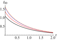
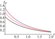
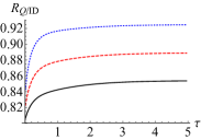
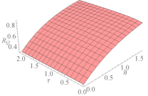
Figure 1: Color online) Upper panels: Performances of the ideal and Q receivers, namely, the mutual informations $I_{ID}$ (left) and Q $I_{Q}$ (right), in the presence of static noise as functions of the phase noise parameter $\tau$ for different seed signals: the solid black line represents the standard coherent state while the dashed red, dotted blue and dotdashed orange lines denote AC states generated respectively with the following NLA’s configurations: $g=1.2,1.6,2$. The input energy of the primary coherent state $\bar{n}=1$. Lower panel in left: The ratio $R_{Q/ID}=I_{Q}/I_{{\scriptscriptstyle I\!D}}$ as a function of $\tau$ for different values of mean photons number: $\bar{n}=0.5$(solid black), $\bar{n}=1$(red dashed) and $\bar{n}=2$(blue dotted). Lower panel in right: 3D plot of the ratio $R_{{\scriptscriptstyle Q}}=I_{c}/I_{{\scriptscriptstyle A\!C}}$ as a function of $\tau$ and $\bar{n}$. The symbols ensemble size is set to $M=20$ in all the plots.

We previously pointed out the optimality-in an ideal transmission line- of the encoding-decoding scheme based on Fock states transmitted following a thermal distribution and photodetection at the stage of the receiver [2]. We recall that the optimisation is performed under a constraint on the mean photons number in the information-bearing system. When it comes to realistic communications, however, the unavoidable presence of noise distorts the transmitted states and alternative encoding-decoding strategies may offer better performances. In fact, for a lossy bosonic channel, it has been shown that an amplitude coherent encoding (usually termed "amplitude-based" scheme), where information is imprinted into the amplitude of coherent states and extracted via heterodyne or double-homodyne detection is indeed optimal. The capacity of the amplitude-based scheme achieved by heterodyne detection is found to be

$$C_{\text{amp}}(\eta)=\log_{2}{(1+\eta\bar{n})},$$ (30)

where $0<\eta<1$ denote the loss parameter and $\bar{n}$ stands for the mean number of photons of the coherent seed state.

In other to deepen our current analysis, we compare the performances of the PSK scheme assisted by the NLA to those of the amplitude-based one. First, we focus on the ideal channel, namely, $\tau=0$ and $\eta=1$. In the right panel of Fig 2, we show the mutual informations for both the ideal $I_{{\scriptscriptstyle I\!D}}$ and the Q receivers $I_{Q}$ along with the capacity of the amplitude-based channel as functions of the mean photons number. We set the symbols ensemble size to $M=20$. Since we intend to establish a comparison between the two channels, the plots are realized for seed signals with equal energies. As it appears from the plots, the two considered schemes afford the same performances in the relevant regime of weak energies ($\bar{n}\ll 1$). However, in the remaining range of $\bar{n}$, the ideal receiver yields some trivial improvement when the average photons number don’t exceed a certain threshold while the Q receiver becomes less efficient as $\bar{n}$ increases.

Let us now compare realistic transmission lines, i.e. phase channels with phase diffusion and amplitude channels with loss. Since the experimental implementation of canonical phase measurement remains unavailable, we will focus on the performances of the $Q$ receiver. In the right panel of Fig 2, we show a 3D plot of the ratio $R_{{\scriptscriptstyle Q}/\text{amp}}=I_{{\scriptscriptstyle Q}}/C_{\text{amp}}$ as a function of the noise parameters $\tau$ and $\eta$ for different values of the mean photons number ($\bar{n}=0.2,1,2$).

The plot reveals the existence of a threshold value of $\bar{n}$, above which the phase channel provides better performances. Moreover, we notice that the region where the phase channel assisted by the NLA outperforms the amplitude-based one becomes larger as the average photons number decreases, thus proving its effectiveness in the relevant regime of weak signals.

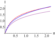
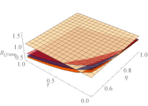
Figure 2: (Color online) Left panel: mutual informations $I_{{\scriptscriptstyle I\!D}}$ (dotted red) and the $I_{{\scriptscriptstyle Q}}$ (dotted purple) receivers together with the capacity of amplitude-based channel (solid blue) as functions of $\bar{n}$ for $M=30$. The considered quantities are evaluated for ideal channels, namely, $\eta=1$ and $\tau=0$. Right panel: 3D plots of the ratio $R_{{\scriptscriptstyle Q}/\text{amp}}=I_{{\scriptscriptstyle Q}}/C_{\text{amp}}$ as a function of $\eta$ and $\tau$ for different values of $\bar{n}$: from top to bottom $\bar{n}=0.2,1,2.$. The number of symbols is set to $M=20$.

5.2 Phase-shift keyed channels in the presence of dynamical noise

The noisy channels considered so far were characterized by a static noise, i.e. a constant phase noise factor. As it happens, the dynamic of the states transferred along the transmission line is well described by a full quantum view under the Markov assumption. In various situations [30, 31, 11, 32, 33], the interaction of the quantum system of interest happens with a structured environment, thus the Markov approximation is no more appropriate. Generally, the theoretical description of quantum systems interacting with correlated in time surrounding degrees of freedom poses real issues. However, when the noise introduced by the environment present classical characteristics-as, for instance, Gaussian noise- the dynamics of the system may be properly modelled by a classical stochastic field (CSF) [34, 35]. Furthermore, beyond its simple formulation, the CSF description enables to investigate the impact of the memory effects induced by the environment on the system.

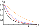
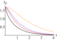
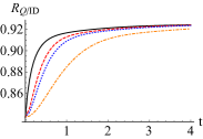
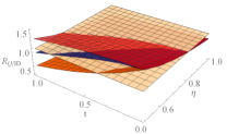
Figure 3: Color online) Upper panels: the mutual information $I_{{\scriptscriptstyle I\!D}}$ (left) and $I_{{\scriptscriptstyle Q}}$ (right) as a function of the interaction time $t$ in the presence of dynamical phase diffusion for different values of the characteristic correlation time $t_{E}$: $t_{E}=0.5$ (dashed red), $t_{E}=1$ (dotted blue),$t_{E}=5$ (dotdashed orange). We also report the plot of the mutual information in the presence of static noise (black solid). Lower left panel: the ratio $R_{{\scriptscriptstyle I\!D}/{\scriptscriptstyle Q}}=I_{{\scriptscriptstyle I\!D}}/I_{{\scriptscriptstyle Q}}$ as a function of $t$ for the same configurations of the upper panels. The colour code is also kept unchanged. Lower right panel: 3D plot of the ratio $R_{{\scriptscriptstyle Q}/\text{amp}}=I_{{\scriptscriptstyle Q}}/C_{\text{amp}}$ as a function of $\eta$ and $t$ for different phase diffusion noises: from bottom to top, static noise, noise with $t_{E}=1$ and noise with $t_{E}=5$. The remaining parameters in all the plots are set as follows: $\bar{n}=2$, $M=20$, $a=3$ and $\Gamma=1$ so as to be consistent with the static case.

In the following, we will address phase communication channels in the presence of dynamical Gaussian noise. We adopt the physical model introduced in Sec 3, where phase diffusion is modelled by a CSF. Given a seed state $\varrho(0)$, the evolved density matrix is given by Eq (15) and can be rewritten as:

$${\varrho}(t)=\int\!d\phi\,\mathcal{N}(\phi,\sigma)\,{U}(\phi)\varrho(0){U}^{\dagger}(\phi)\,,$$ (31)

where $\mathcal{N}(\phi,\sigma)$ is a normal distribution with zero mean and a time-dependant variance $\sigma(t)$. It entirely characterizes the stochastic Gaussian process (CSF) and is directly related to its autocorrelation function through Eq. (14) . The transformation (31) induced by the environment, takes an initial state $\varrho(0)$ to a statistical mixture of phase-shifted states distributed according to a Normal law around its initial phase. In the following, we will treat the case of the power-law (PL) process as an illustrative pattern of Gaussian CSF. The PL process is characterized by the kernel $K(t,t^{\prime})=\frac{a-1}{2}\frac{\gamma\Gamma}{\left(1+\gamma\left|t-t^{\prime}\right|\right)^{a}}$, where $\Gamma$ stands for the phase diffusion parameter and $\gamma=t_{E}^{-1}$, with $t_{E}$ being the correlation time of the environment. As it happens, for a null central frequency of the environment ($\omega=0$) the time-dependant variance $\sigma(t)$ reads

$$\sigma_{PL}(t)=\frac{\Gamma}{\gamma}\left[\frac{(1+\gamma t)^{2-a}+\gamma t(a-2)-1}{a-2}\right].$$ (32)

In the limit where $\gamma\rightarrow\infty$, or equivalently, the environment’s correlation time is negligible with respect to the interaction time ($t_{E}\ll t$), the variance reduces to

$$\sigma_{PL}(t)\simeq\Gamma t,$$ (33)

whereas for vanishing $\gamma$, namely, in the presence of consequential memory effects ($t_{E}\gg t$), it assumes the following form

$$\sigma_{PL}(t)\simeq\frac{\Gamma t^{2}}{2}\left(a-1\right),$$ (34)

As it appears from Eq (33), where the variance is linear in time, we are back to the static situation where memory effects are negligible, and the CSF is well described in the Markovian approximation, thereby, the mutual information shows the same behaviour as in Fig 2.

Let us now analyze the impact of memory effects on the information transferred along a phase diffusive channel. The mutual informations for both the ideal and the Q receiver are evaluated by performing the replacement $e^{-\frac{1}{2}d^{2}\tau}\rightarrow e^{-\frac{1}{2}d^{2}\sigma(t)}$ in the expressions (28) and (29) respectively. In the upper panels of Fig 3, we report variations of the mutual informations $I_{{\scriptscriptstyle I\!D}}$ and $I_{{\scriptscriptstyle Q}}$ with respect to the interaction time $t$ for different values of the environment’s correlation time $t_{E}$. For the sake of comparison, we also show the mutual information for the static phase noise. The plots reveal better performances for both the ideal and Q receiver in the presence of dynamical noise. Moreover, we observe that the larger is the correlation time, better preserved is the mutual information. In fact, the decay rate drops for consequential memory effects whereas being at its maximum for vanishing $t_{E}$ as illustrated by the transition (Eq(33)$\rightarrow$ (Eq(34))) from linear to quadratic variations in time of $\sigma(t)$. In the lower panel, right side, we show the ratio $R_{{\scriptscriptstyle Q}/{\scriptscriptstyle I\!D}}=I_{{\scriptscriptstyle Q}}/I_{{\scriptscriptstyle I\!D}}$ as a function of the interaction time $t$ for different values of $t_{E}$. We observe a decreasing ratio with respect to the correlation time, denoting that the dynamical phase noise disadvantages the Q receiver compared with the ideal one.

Let us now compare the performances to those of an amplitude-based channel in the presence of noise. Once again, we consider a dynamical noise originated from a long range power-Law process. Our results are depicted in the lower right panel of Fig 3, where we show a 3D plot of the ratio $R_{{\scriptscriptstyle Q}/\text{amp}}=I_{{\scriptscriptstyle Q}}/C_{\text{amp}}$ as a function of the amplitude loss parameter $\eta$ and the interaction time $t$, for two values of the correlation time of the environment ($t_{E}=1,5$). In order to emphasize the contribution coming from the memory effects, we also report the 3D plot of the ratio in the presence of static noise. It is worth noting that we have considered here the regime of weak energies ($\bar{n}=0.2$). We clearly notice that the environment memory effects enhance the performances of the noisy phase-based channel assisted by the NLA with respect to the amplitude-based one. This is illustrated by the increased area where the phase channel outperforms its amplitude counterpart for higher time-correlated environments. Overall, we conclude that memory effects are a resource to preserve information in the presence of phase diffusion.

6 Conclusion

We have investigated quantum phase communication channels assisted by probabilistic noiseless linear amplification and assessed their performances in presence of static and dynamical phase noise.

At first, we have shown that in the presence of Markovian noise, NL-amplification of the coherent seed signal improves the performances for both ideal and feasible receivers. Moreover, upon comparison with lossy coherent states amplitude-based scheme we have shown the existence of a threshold on the loss and phase noise parameters, above which phase channels better preserve the transfer of information. Then, we have shown that in the presence of time-correlated noise, leading to dynamical non-Markovian phase diffusion, the interplay between the use of NLA and the memory effects provide a noticeable improvement of performances, i.e memory effects better preserve the information transferred along the transmission line.

Overall, our results prove that quantum phase communication channels may be of interest for applications with current technology, and pave the way for their implementations in realistic scenarios.

References

- [1] A. S. Holevo and R. F. Werner, “Evaluating capacities of bosonic gaussian channels,” Phys. Rev. A 63, 032312 (2001).
- [2] H. P. Yuen and M. Ozawa, “Ultimate information carrying limit of quantum systems,” Phys. Rev. Lett. 70, 363–366 (1993).
- [3] V. Giovannetti, S. Guha, S. Lloyd, L. Maccone, J. H. Shapiro, and H. P. Yuen, “Classical capacity of the lossy bosonic channel: The exact solution,” Phys. Rev. Lett. 92, 027902 (2004).
- [4] V. Giovannetti, S. Guha, S. Lloyd, L. Maccone, J. Shapiro, B. J. Yen, and H. P. Yuen, “Classical capacity of free-space optical communication,” Quantum Inf. Comp. 4, 489 (2004).
- [5] R. Nair, B. J. Yen, S. Guha, J. H. Shapiro, and S. Pirandola, “Quantum m-ary phase shift keying,” in “2012 IEEE International Symposium on Information Theory Proceedings,” (2012), pp. 556–560.
- [6] G. M. D’Ariano, C. Macchiavello, N. Sterpi, and H. P. Yuen, “Quantum phase amplification,” Phys. Rev. A 54, 4712–4718 (1996).
- [7] S. Olivares, S. Cialdi, F. Castelli, and M. G. A. Paris, “Homodyne detection as a near-optimum receiver for phase-shift-keyed binary communication in the presence of phase diffusion,” Phys. Rev. A 87, 050303 (2013).
- [8] M. G. Genoni, S. Olivares, and M. G. A. Paris, “Optical phase estimation in the presence of phase diffusion,” Phys. Rev. Lett. 106, 153603 (2011).
- [9] B. Teklu, J. Trapani, S. Olivares, and M. G. A. Paris, “Noisy quantum phase communication channels,” Physica Scripta 90, 074027 (2015).
- [10] J. Trapani, B. Teklu, S. Olivares, and M. G. A. Paris, “Quantum phase communication channels in the presence of static and dynamical phase diffusion,” Phys. Rev. A 92, 012317 (2015).
- [11] R. Vasile, S. Olivares, M. A. Paris, and S. Maniscalco, “Continuous-variable quantum key distribution in non-markovian channels,” Phys. Rev. A 83, 042321 (2011).
- [12] C. M. Caves, “Quantum limits on noise in linear amplifiers,” Phys. Rev. D 26, 1817–1839 (1982).
- [13] J. Fiurášek, “Engineering quantum operations on traveling light beams by multiple photon addition and subtraction,” Phys. Rev. A 80, 053822 (2009).
- [14] A. Zavatta, J. Fiurášek, and M. Bellini, “A high-fidelity noiseless amplifier for quantum light states,” Nature Photonics 5, 52 (2011).
- [15] T. Ralph and A. Lund, “Nondeterministic noiseless linear amplification of quantum systems,” in “AIP Conference Proceedings,” , vol. 1110 (AIP, 2009), vol. 1110, pp. 155–160.
- [16] M. A. Usuga, C. R. Müller, C. Wittmann, P. Marek, R. Filip, C. Marquardt, G. Leuchs, and U. L. Andersen, “Noise-powered probabilistic concentration of phase information,” Nature Physics 6, 767 (2010).
- [17] F. Ferreyrol, M. Barbieri, R. Blandino, S. Fossier, R. Tualle-Brouri, and P. Grangier, “Implementation of a nondeterministic optical noiseless amplifier,” Phys. Rev. Lett. 104, 123603 (2010).
- [18] N. A. McMahon, A. P. Lund, and T. C. Ralph, “Optimal architecture for a nondeterministic noiseless linear amplifier,” Phys. Rev. A 89, 023846 (2014).
- [19] S. Pandey, Z. Jiang, J. Combes, and C. M. Caves, “Quantum limits on probabilistic amplifiers,” Phys. Rev. A 88, 033852 (2013).
- [20] S. Olivares and M. G. A. Paris, “Photon subtracted states and enhancement of nonlocality in the presence of noise,” Journal of Optics B: Quantum and Semiclassical Optics 7, S392–S397 (2005).
- [21] J. Fiurášek, and N. J. Cerf, “Gaussian postselection and virtual noiseless amplification in continuous-variable quantum key distribution,” Phys. Rev. A 86, 060302 (2012).
- [22] N. Walk, T. C. Ralph, T. Symul, and P. K. Lam, “Security of continuous-variable quantum cryptography with Gaussian postselection,” Phys. Rev. A 87, 020303 (2013).
- [23] H. M. Chrzanowski, N. Walk, S. M. Assad, J. Janousek, S. Hosseini, T. C. Ralph, et al. “Measurement-based noiseless linear amplification for quantum communication,” Nature Photonics, 8, 333 (2014).
- [24] U. Leonhardt, J. A. Vaccaro, B. Böhmer, and H. Paul, “Canonical and measured phase distributions,” Phys. Rev. A 51, 84–95 (1995).
- [25] M. G. A. Paris, “Sampling canonical phase distribution,” Phys. Rev. A 60, 5136–5139 (1999).
- [26] J. W. Noh, A. Fougères, and L. Mandel, “Measurement of the quantum phase by photon counting,” Phys. Rev. Lett. 67, 1426–1429 (1991).
- [27] G. M. D’Ariano and M. G. A. Paris, “Lower bounds on phase sensitivity in ideal and feasible measurements,” Phys. Rev. A 49, 3022–3036 (1994).
- [28] N. D. Pozza and M. G. A. Paris, “An effective iterative method to build the naimark extension of rank-n povms,” International Journal of Quantum Information 15, 1750029 (2017).
- [29] N. Dalla Pozza and M. G. A. Paris, “Naimark extension for the single-photon canonical phase measurement,” arXiv e-prints arXiv:1904.00632 (2019).
- [30] M. J. Biercuk, H. Uys, A. P. VanDevender, N. Shiga, W. M. Itano, and J. J. Bollinger, “Optimized dynamical decoupling in a model quantum memory,” Nature 458, 996 (2009).
- [31] A. W. Chin, S. F. Huelga, and M. B. Plenio, “Quantum metrology in non-markovian environments,” Phys. Rev. Lett. 109, 233601 (2012).
- [32] R. Schmidt, A. Negretti, J. Ankerhold, T. Calarco, and J. T. Stockburger, “Optimal control of open quantum systems: Cooperative effects of driving and dissipation,” Phys. Rev. Lett. 107, 130404 (2011).
- [33] M. Thorwart, J. Eckel, J. Reina, P. Nalbach, and S. Weiss, “Enhanced quantum entanglement in the non-markovian dynamics of biomolecular excitons,” Chemical Physics Letters 478, 234 – 237 (2009).
- [34] W. M. Witzel, K. Young, and S. Das Sarma, “Converting a real quantum spin bath to an effective classical noise acting on a central spin,” Phys. Rev. B 90, 115431 (2014).
- [35] J. Trapani, M. Bina, S. Maniscalco, and M. G. A. Paris, “Collapse and revival of quantum coherence for a harmonic oscillator interacting with a classical fluctuating environment,” Phys. Rev. A 91, 022113 (2015).