Let’s deflate that beach ball

Abstract

We investigate the relationship between pre-buckling and post-buckling states as a function of shell properties, within the deflation process of shells of an isotropic material. With an original and low-cost set-up that allows to measure simultaneously volume and pressure, elastic shells whose relative thicknesses span on a broad range are deflated until they buckle. We characterize the post-buckling state in the pressure-volume diagram, but also the relaxation toward this state. The main result is that before as well as after the buckling, the shells behave in a way compatible with predictions generated through thin shell assumption, and that this consistency persists for shells where the thickness reaches up to 0.3 the shell’s midsurface radius.

1 Introduction

Due to the boom of microfluidics and miniaturization, small spherical objects are increasingly studied in soft matter, many of them thin and prone to deformation. Deformation is usually accompanied by deflation (e.g. due to osmotic pressure, or leakage, or lateral expansion of the shell). There have been several theoretical or numerical studies Hutchinson 1967 ; LandauBook ; Quilliet2008 ; Quilliet2008err ; Knoche2011 ; Vliegen2011 ; Quilliet_2012 ; Hutchinson_2017 ; pezzulla2018 and some experimental investigations Carlson_1967 ; Carlson_1968 ; Zhang_2017 about the deflation of a thin, elastic, shell. Most of them focus essentially on understanding and quantifying the scenario of the buckling instability that occurs beyond a certain threshold of compression or deflation. Less is known about the post-buckling behaviour Quilliet2008 ; Quilliet2008err ; Knoche2011 ; Quilliet_2012 ; Knoche2014 , let alone when thin shell theory is a priori not valid. It is generally assumed that a 2D description of the shell is valid when $d/R<0.02$, where $d$ is the shell thickness and $R$ its mid-surface radius ($R-\frac{d}{2}$ and $R+\frac{d}{2}$ are then respectively the internal and external radii). In that case the 2D properties of the surface model can be interpreted in terms of shell thickness and 3D properties of the constituting material. These models indeed constitute a simplification compared to studies managing 3D features Church_1994 ; Knoche2011 .

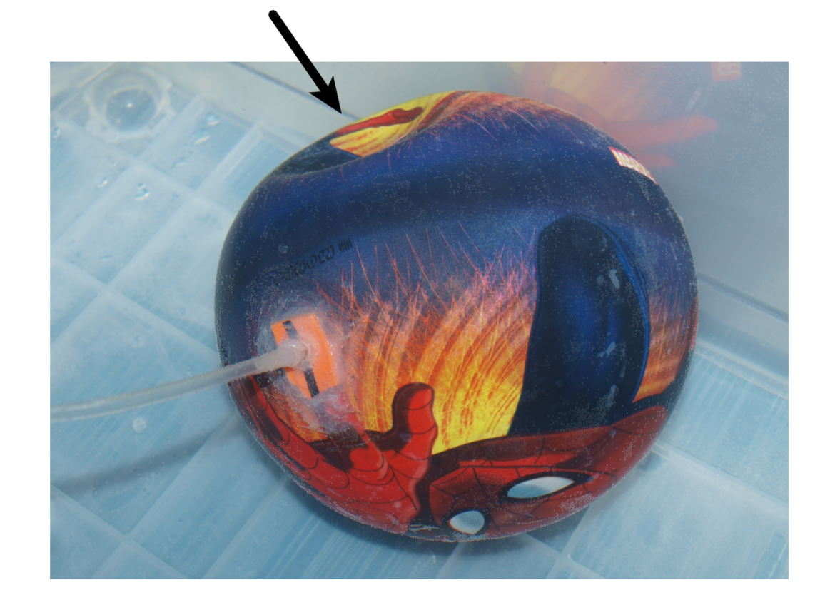
Figure 1: Buckled shell through volume loss: an axisymmetric depression (shown by arrow) suddenly appears when internal volume is slowly decreased. External radius $R+d/2=171$ mm; relative thickness $d/R=6.5\thinspace 10^{-3}$.

In this paper, we investigate experimentally the deflation of elastic macroscopic shells, down to buckling and post-buckling deformations, for a broad range of relative shell thicknesses. These results are compared to what is known from thin shell theory, which allows to discuss its validity range.

Our low-cost experimental set-up was conceived as an efficient and versatile tool for exploring with students instability issues and bifurcations diagrams under several conditions (volume or pressure imposed), and for characterizing shells before using them in a more complex environment Djellouli_2017 . Yet, it provides for the first time an experimental characterization of the relationship between pre-buckling and post-buckling states. Transition between these two states is accompanied by a fast release of energy, a feature present in Nature forterre05 ; vincent11 ; son2013 that has already been used in several applications with similar soft systems Djellouli_2017 ; holmes07 ; yang15 ; ramachandran2016 ; gomez2017 ; holmes2019 .

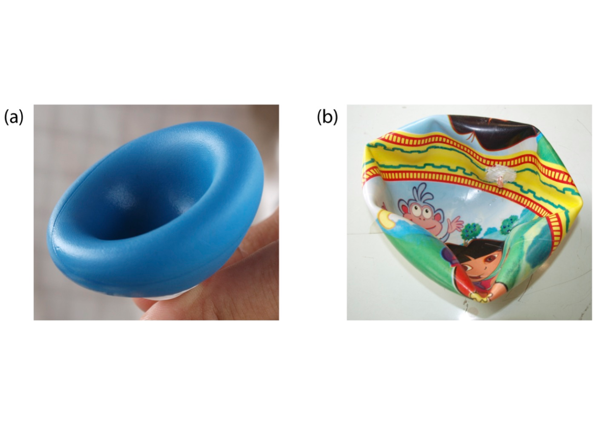
Figure 2: Elastic shells almost fully deflated; the hemisphere that is curved inward is in contact with the, mainly unchanged, other half of the shell. (a) Thick shell (relative thickness $d/R=0.18$; external radius $R+d/2=55.5\,\mathrm{mm}$), in which axisymmetry was conserved throughout the deflation. (b) Thin shell ($d/R=10.6\thinspace 10^{-3}$; external radius $R+d/2=190\,\mathrm{mm}$), where radial folds began to develop inside the depression at some point of the deflation process.

Spherical shells of an isotropic elastic material are expected to undergo sequences of shapes that depend only on intensive parameters: Poisson’s ratio $\nu$ and relative thickness $d/R$. Shells should first stay spherical while their radius decreases, up to the point where a buckling instability suddenly makes a circular depression appear, of characteristic dimension $\sqrt{dR}$ (Fig. 1) LandauBook ; Pogorelov . This step was only recently understood in terms of mode localization Hutchinson_2017 ; Hutchinson_2016 . According to simulations and theoretical studies, the depression then grows axisymmetrically when the shell is slowly deflated Quilliet2008 ; Quilliet2008err ; Knoche2011 ; Hutchinson_2017 . Thicker shells keep axisymmetry up to self-contact (Fig. 2-a), while for thinner shells, the depression looses its axisymmetry during deflation, progressively developing radial folds (Fig. 2-b) Quilliet2008 ; Quilliet2008err ; Quilliet_2012 ; Hutchinson_2017 ; Knoche2014 .

Quantitatively, the deflation is characterized by the volume change $\Delta V$ from the initial nondeflated state, and the pressure drop $\Delta P=P_{ext}-P_{int}>0$ it induces between both sides of the shell (outside and inside the ball). In a surface model, the denominator of the dimensionless relative volume variation $\frac{\Delta V}{V_{0}}$ is the volume enclosed by the initial undeformed surface. For this experimental study we chose to take as a reference the volume $V_{0}=\frac{4}{3}\pi R^{3}$ initially enclosed by the midsurface of the shell, instead of the volume $V_{int}=\frac{4}{3}\pi\left(R-\frac{d}{2}\right)^{3}$ effectively contained in the shell, thus allowing direct comparison with surface models. The set-up we developed provides the pressure drop and the volume variation of deflated spheres of known initial volume ; we could then follow and discuss deformation paths observed in a $\Delta P\,-\,\frac{\Delta V}{V_{0}}$ diagram. We denote by $\wp(\frac{\Delta V}{V_{0}})$ the state equation between both quantities at equilibrium. This function $\wp$ is to be determined in this paper.

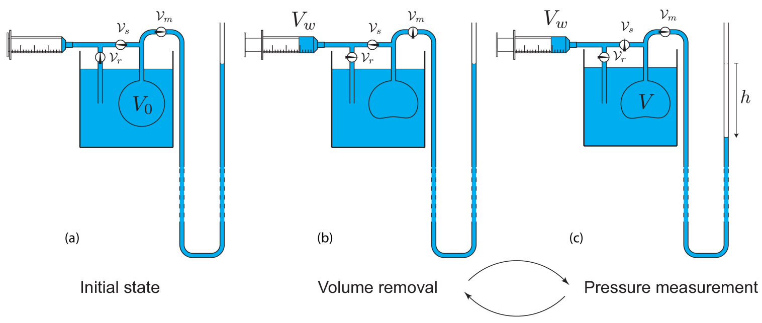
Figure 3: Principle of the experiment: an elastomer ball is plunged in a tank of water. The ball is filled with the same liquid, which avoids extra deformations due to internal-external differences of hydrostatic pressure. Its inner volume is linked either to a manometer (U tube on the right) through valve $\mathcal{V}_{m}$, or, through valve $\mathcal{V}_{s}$, to a syringe that modifies the volume whatever the pressure, or to the water tank through valves $\mathcal{V}_{s}$ and $\mathcal{V}_{r}$. (a) Initial state: pressures in the ball, in the manometer and in the water tank are equilibrated ($\mathcal{V}_{m}$, $\mathcal{V}_{s}$ and $\mathcal{V}_{r}$ open). The initial volume enclosed by its midsurface is $V_{0}=\frac{4}{3}\pi R^{3}$ (reference for subsequent calculation of the relative volume variation). At rest, the level in the manometer (which is a tiny tube) overtakes that in the tank by about a few millimeters, due to capillary effects. This level at rest is taken as the reference for pressure calculations. (b) Deflation: through open $\mathcal{V}_{s}$, the syringe removes a controlled volume of water $\delta V_{i}$ (this volume can safely be considered as incompressible even if inner pressure drastically drops). (c) After the closing of $\mathcal{V}_{s}$, the opening of $\mathcal{V}_{m}$, and equilibration, the pressure difference between both sides of the ball wall is calculated from the slump $h>0$ of water level in the manometer: $\Delta P=\rho gh$. The inner volume change due to the level adjustment in the manometer is not negligible and is taken into account in further calculations. Practically, deflation is done stepwise, through repetition of stages (b) and (c), this latter providing a series of equilibrium states corresponding to inner volume variations $\left(\Delta V_{1},...,\Delta V_{i},\Delta V_{i+1},...\right)$. When full, the syringe can be emptied through valve $\mathcal{V}_{r}$ without opening the system.

2 Set-up for deflation experiments

We considered about 25 commercial hollow balls (beach balls, squash balls, juggle balls, balls for rhythmic gymnastics…) made of elastomers, of external radii $R+d/2$ ranging between 39.5 and 190 mm, and $d/R$ ratios between $6.5\thinspace 10^{-3}$ and 0.25, plus a homemade ball of relative thickness 0.22 Djellouli_2017 . All Young moduli $Y_{3D}$ measured for small strains are between 0.5 and 7.5 MPa (see section 4).

In order to easily measure volumes and pressures, the ball is filled with an incompressible fluid (water). It is then also immersed in water so as to avoid gradients of hydrostatic pressure along the ball (which amounts to study shapes not deformed by gravity). The ball is connected to a U-shape manometer, a syringe, and a third tube connected to the tank of water so as to favor initial quick equilibration of all pressures (Fig. 3-a). In the initial state, the pressure difference $\Delta P$ is 0. Taps allow us to connect the ball either to the syringe or to the manometer. The manometer is made of a cylindrical tube of diameter ranging between 0.79 and 3.18 mm and thick enough to avoid tube buckling under the highest pressure differences 1 bar, which are met with thick squash balls. If required, the total height of the manometer could reach $10\,\mathrm{m}$ so as to measure such depressions.

The experiment is run as follows: an increasing amount of liquid $\Delta V_{w}$ is withdrawn from the ball through valve $\mathcal{V}_{s}$ (Fig. 3-b), via small volume intakes $\delta V_{i}$ ($\Delta V_{w}=\sum\delta V_{i}$). After each step the ball is put in contact with the sole manometer through valve $\mathcal{V}_{m}$. The displacement $h>0$ of the liquid in the manometer from the initial equilibrium situation yields the pressure difference $P_{ext}-P_{int}=\rho gh$ across the ball membrane, where $\rho$ is the density of water. Because of the fluid volume variations in the manometer, the inner volume variation $\Delta V$ of the shell is slightly different from the volume $\Delta V_{w}$ set through the syringe :

$$\Delta V=\Delta V_{w}-\pi r^{2}h,$$ (1)

where $r$ is the internal radius of the (cylindrical) manometer tube. Even though this correction is systematically taken into account, the problem with large sections $S=\pi r^{2}$ would be that the volume withdrawn in the syringe has to be much larger than the targeted $\Delta V$, which may possibly make the system jump to another stability branch. This could impede full characterization of the branch of interest ; this is discussed in detail in subsection 3.2.2. On the other hand, the limitation when decreasing $S$ lies in a possibly high equilibration time (see subsection 3.2.1). These experimental precautions being taken into account, for each ball the pressure difference $\Delta P$ at mechanical equilibrium can be plotted with respect to the relative volume variation $\frac{\Delta V}{V_{0}}$, giving insights on the state equation $\wp(\frac{\Delta V}{V_{0}})$ that is expected to depend on the relative thickness $d/R$ of the ball, and on its material’s properties ($Y_{3D}$, $\nu$).

The two-step procedure ensures to work at almost imposed volume and to discuss the time evolution of the system from a known state. Had the valves $\mathcal{V}_{s}$ and $\mathcal{V}_{m}$ always been kept open so as to measure simultaneously volumes and pressures, the interpretation of the dynamics towards equilibrium would have been more tricky, since sucking out fluids in the manometer amounts to imposing pressure in the shell once the withdrawal step is stopped. The relative contribution of the volume withdrawal in the shell and in the manometer would depend on the whole set-up configuration, and in particular on the tubings resistance, as well as on the shell mechanical properties.

3 Deflation of spherical shells

Deflation essentially occurs within two regimes. In a first mode of deformation, the ball roughly keeps its sphericity. Then a sudden transition LandauBook ; Knoche2011 ; Quilliet_2012 ; Hutchinson_2017 ; Church_1994 ; Hutchinson_2016 transforms the sphere into an axisymmetric shape with a dimple (Fig. 1). Further deflation makes the dimple size continuously increase (Fig. 2-a) Knoche2011 ; Quilliet_2012 ; Hutchinson_2017 . Note that quick deflation can lead to multi-dimple deformations, which were shown to correspond to branches of higher energy Quemeneur2012 , but this was not observed thanks to our small-stepped-deflation.

3.1 Linear regime before buckling

The first regime corresponds to constraints with a spherical symmetry, which results in a “in-plane” compression of the shell (i.e. parallel to the free surfaces). For materials with nonzero Poisson’s ratio, this induces elongationnal shear in the thickness of the shell but, in the surface model that is used to describe thin shells, spherical shrinking can be modelled by a uniform in-plane compression of a spherical surface Quilliet_2012 . In a $\Delta P$ versus $\frac{\Delta V}{V_{0}}$ diagram, quadratic compression energy corresponds to a linear evolution Quilliet_2012 ; Marmottant_2011 : $\Delta P=\frac{4\chi_{2D}}{3R}\left(\frac{\Delta V}{V_{0}}\right)$, where $\chi_{2D}$ is the surface compression modulus. For a thin shell of an isotropic material, this 2D effective parameter can be linked to the 3D properties of the shell through $\chi_{2D}=\frac{Y_{3D}d}{2\left(1-\nu\right)}$, where $Y_{3D}$ is the Young modulus of the material, and $\nu$ its Poisson’s ratio ($\nu\lesssim 0.5$ for most of the elastomeric materials, these latter being exclusively used for our experiments because they can undergo a 200% elongation without plastic deformation or fracturation). Hence:

$$\Delta P=\frac{2Y_{3D}}{3\left(1-\nu\right)}\times\frac{d}{R}\left(\frac{\Delta V}{V_{0}}\right).$$ (2)

Experiments effectively show the expected linear behaviour, as exemplified in Fig. 4. Values of the slope are used to nondimensionalise the characteristic post-buckling pressures in subsection 3.2.4, and are compared in section 4 to traction experiments which provided independent measurements of $Y_{3D}$ and $\nu$.

This linear regime persists up to the point where an instability causes a drastic change of shape (”buckling”) toward a configuration with a single axisymmetric dimple, together with a drop of $\Delta P$. The critical pressure at which buckling takes place was predicted from classical buckling theory Hutchinson 1967 ; Knoche2011 to be:

$$\Delta P_{c}=\frac{2}{\sqrt{3\left(1-\nu^{2}\right)}}\times Y_{3D}\left(\frac{d}{R}\right)^{2}.$$ (3)

In experiments, buckling often occurs before this threshold is reached, because of defects in the material Vella2011 ; Reis2017 , possibly down to 20% of the theoretical predictions for a perfect shell Hutchinson_2016 .

According to numerical studies Knoche2011 ; Quilliet_2012 ; Marmottant_2011 , proceeding with small deflation steps after this buckling hardly changes the value of $\Delta P$, which roughly plateaus during a substantial range of $\frac{\Delta V}{V_{0}}$. Plateauing, which is exemplified in Fig. 4-b is specifically studied in the next section. For the thinnest shells, further deflation steps lead to a second, softer transition where radial folds progressively appear in the dimple (see Fig. 2-b and refs. Quilliet2008 ; Quilliet2008err ; Quilliet_2012 ) ; this aspect is not addressed in the present paper.

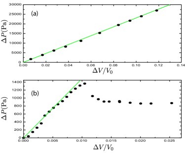
Figure 4: Outside-inside pressure difference $\Delta P=P_{ext}-P_{int}$ for different elastic shells, versus the relative volume variation. All measurements done at equilibrium for different water volume removals are represented. Green line: linear fit before buckling. (a) $R=22.5$ mm, $d/R=0.222,$ $Y_{3D}=0.5$ MPa (measured by traction experiments, see subsection 4). (b) $R=51.2$ mm, $d/R=0.0293$, $Y_{3D}=5.5$ MPa. Buckling can be observed here for $\frac{\Delta V}{V_{0}}\,\apprge\,0.01$, and plateauing (see subsection 3.2) for $\frac{\Delta V}{V_{0}}$ over about 0.015.

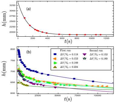
Figure 5: ”Slow devices”: Time evolution of the slump $h$ of water level in the manometer. (a) Monoexponential relaxation with a characteristic time $\tau=129$ s for a ball of radius $R=22.5$ mm and relative thickness $d/R=0.222$; relative volume variation after stabilization (i.e. calculated using $h_{asympt}$ in Eq. (1)) $\frac{\Delta V_{asympt}}{V_{0}}=0.211$. (b) Biexponential relaxation for different values of the volume sucked out from a ball of radius $R=58.7$ mm and $d/R=0.097$, during 2 different sequences of deflation. All theoretical curves correspond to a biexponential fit with the same pair of characteristic times ($\tau_{1}=440$ s, $\tau_{2}=15000$ s) and the same proportion $p=0.42$ of short-time exponential.

3.2 Post-buckling plateau

3.2.1 Stabilization time

During the spherical mode of deflation, the water level continuously falls (stabilizing within a few seconds) every time a small amount of water is sucked out from the ball. After buckling, it suddenly rises in the manometer. When deflation is performed further on, several behaviours may take place:

- For most ball+manometer devices, the water level in the manometer stabilizes within a few seconds at each post-buckling deflation step. When recorded for a large range of relative volume variations, the slump $h$ under the reference equilibrium level in the manometer hardly varies with $\frac{\Delta V}{V_{0}}$ (”plateauing”). It shows indeed a very weak minimum at some intermediate value (as examplified in fig. 4-b for $\frac{\Delta V}{V_{0}}$ above 0.015). Then, for the experiments carried at sufficiently large deflation, it re-increases which corresponds to an expected divergence when $\frac{\Delta V}{V_{0}}$ approaches 1 (ideally emptied ball)Knoche2011 . The minimum value $h{}_{min}$ of $h$ when it plateaus allows to determine the so-called ”plateauing pressure” $\Delta P_{pl}=\rho gh_{min}$. This quantity underwent a specific study in the numerical simulations of ref. Quilliet_2012 , which will be revisited hereafter.

- Nevertheless, for some ball+manometer devices, at all deflation steps $h$ systematically shows a steep increase (i.e. the water level is suddenly sucked down for a few seconds) every time the ball is reconnected to the manometer after the sucking out of $\delta V_{i}$; then it decreases during minutes or more before stabilization, down to a new equilibrium value $h_{asympt}$. In the following, these experimental configurations are named ”slow devices”. For most shells where post-buckling equilibrium is not immediately realized, it would have been too long to wait for $h$ reaching the $h_{asympt}$ value for each relative volume variation $\frac{\Delta V}{V_{0}}$ explored. Fortunately, we found out that the decrease of $h(t)$ was exponential for a few cases (fig. 5-a), and that in the other cases it could be fitted using a biexponential of general formula:

$$h\left(t\right)=h_{asympt}+\left(h_{init}-h_{asympt}\right)\left[p\,e^{-t/\tau_{1}}+\left(1-p\right)e^{-t/\tau_{2}}\right],$$ (4)

where $\tau_{1}$ and $\tau_{2}$ are respectively the short and long characteristic times, and $p$ the proportion of short-time exponential in the modelled signal (see Fig. 5-b).

Mechanical equilibrium is realized only when the water level in the manometer reaches its asymptotic value $h_{asympt}$. The $\left(\frac{\Delta V}{V_{0}},\Delta P=\rho gh_{asympt}\right)$ experimental graph shows plateauing as for balls without time delay. Results are presented and discussed in subsection 3.2.4.

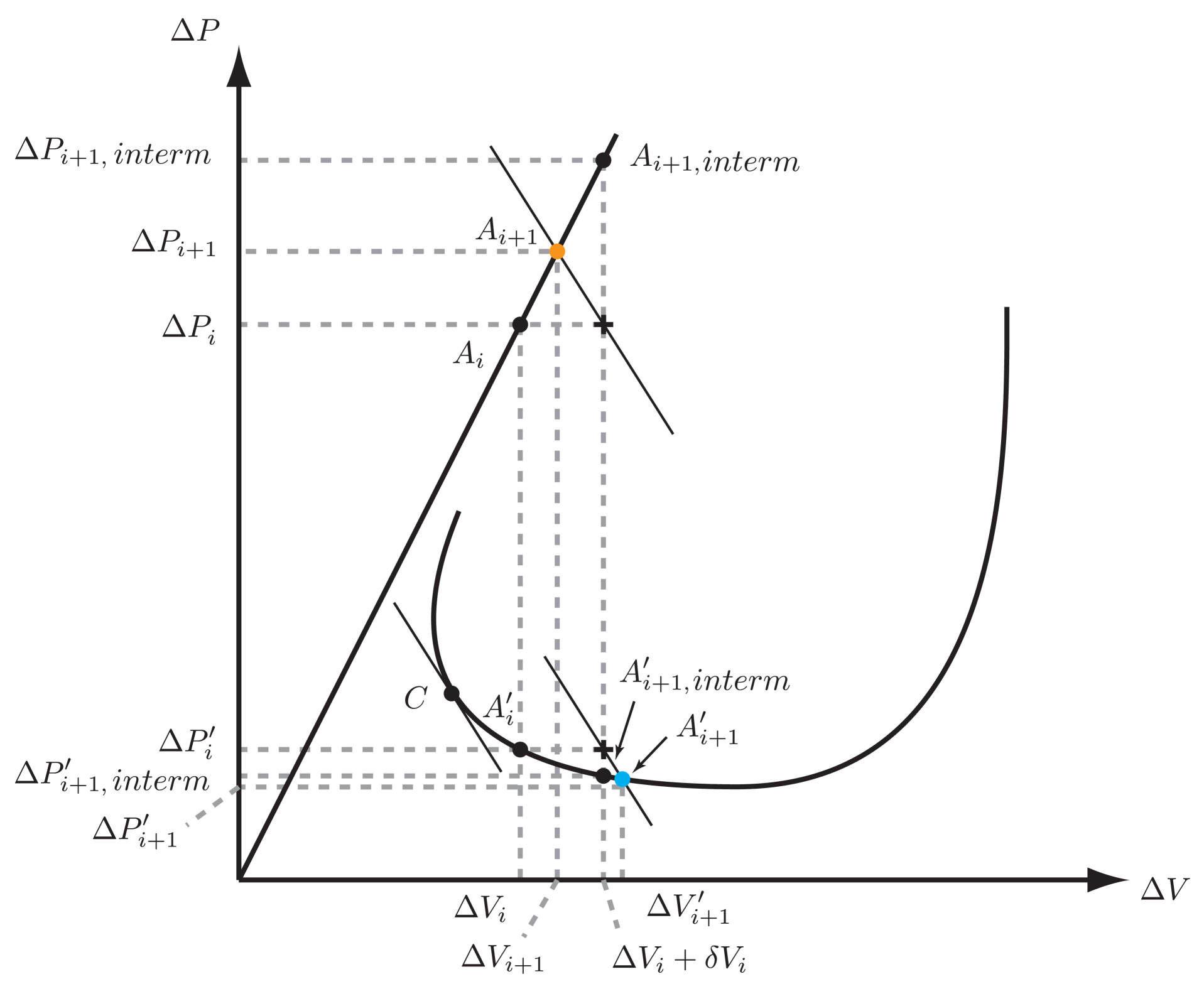
Figure 6: Continuous black lines: typical state function (see Knoche2011 ; Quilliet_2012 ), that can locally be denotated as $\wp(\Delta V)$. Upper branch: after removal of a volume of water $\delta V_{i}$ (with the syringe through valve $\mathcal{V}_{s}$) from the equilibrium state $A_{i}\left(\Delta V_{i},\Delta P_{i}\right)$, the shell finds a non-observable intermediate equilibrium state $A_{i+1,interm}\left(\Delta V_{i}+\delta V_{i},\Delta P_{i+1,interm}\right)$. Opening valve $\mathcal{V}_{m}$ for the measurement of the inner pressure leads to a new (observable) equilibrium state $A_{i+1}\left(\Delta V_{i+1},\Delta P_{i+1}\right)$, in orange, at the intersection of $\wp(\Delta V)$ and the straight line of slope $\left(-\frac{\rho g}{\pi r^{2}}\right)$ (cf Eq. (5)) that passes through the point $\left(\Delta V_{i}+\delta V_{i},\Delta P_{i}\right)$). Since $\frac{d\wp}{d(\Delta V)}>0$, one gets $\Delta V_{i+1}<\Delta V_{i}+\delta V_{i}$. Lower branch: same construction (with primed symbols) for intermediate and final state (in blue). As $\frac{d\wp}{d(\Delta V)}<0$ there, the inequality reverts: $\Delta V_{i+1}>\Delta V_{i}+\delta V_{i}$. This construction shows that on the lower stability branch, states corresponding to a $\Delta P$ higher than in state C, where the slope equals to $\left(-\frac{\rho g}{\pi r^{2}}\right)$, cannot be explored.

3.2.2 Equilibrium and manometer

The equilibrium configurations, and the route toward them, are obtained while the shell is in contact with the manometer. In the two following subsections, we establish how this coupling influences the way the state diagram is explored and how the dynamical features intrinsic to the shell can be extracted.

After closing of valve $\mathcal{V}_{s}$ and opening of valve $\mathcal{V}_{m}$ (see Fig. 3), pressure adaptation between the ball and the manometer occurs through water exchange, which in turn modifies (i) the pressure exerted by the water column in the ball (ii) the volume of the ball, hence the pressure exerted by the shell. The final state emerges from this feedback. Two characteristic situations are displayed in Fig. 6. After a volume $\delta V_{i}$ has been sucked out from a ball at equilibrium with state $\left(\Delta V_{i},\Delta P_{i}\right)$, the ball finds itself in a state $\left(\Delta V_{i}+\delta V_{i},\Delta P_{i+1,interm}\right)$, which we assume here to be an equilibrium state. Nevertheless, features of this new state are not known by the experimentalist, who has to open valve $\mathcal{V}_{m}$ in order to measure the pressure. Once the ball and manometer are in contact, the pressure difference $\Delta P_{i+1,interm}$ between both extremities of the manometer is not a priori equilibrated by the water withdrawal $h_{i}$ (that previously equilibrated $\Delta P_{i}$). This leads to a flow in the manometer until the outside-inside pressure difference $\Delta P=P_{ext}-P_{int}$ is equilibrated by the hydrostatic pressure associated with withdrawal $h$: $\Delta P_{i}-\Delta P=\rho g\left(h_{i}-h\right)$. On an other hand, conservation of water volume implies that $\Delta V-\Delta V_{i}=\delta V_{i}-\pi r^{2}\left(h-h_{i}\right)$; hence:

$$\Delta P=\Delta P_{i}+\frac{\rho g}{\pi r^{2}}\left(\Delta V_{i}+\delta V_{i}-\Delta V\right).$$ (5)

In a $\Delta P-\Delta V$ diagram, this is the equation of the straight line (”operating curve”) of slope $\left(-\frac{\rho g}{\pi r^{2}}\right)$ that passes through the point $\left(\Delta V_{i}+\delta V_{i},\Delta P_{i}\right)$ (Fig. 6). The measured equilibrium state $\left(\Delta V_{i+1},\Delta P_{i+1}\right)$ is then found by following the state curve $\wp(\Delta V)$ from the intermediate equilibrium state (with valve $\mathcal{V}_{m}$ closed) $(\Delta V_{i}+\delta V_{i},\Delta P_{i+1,interm})$ up to its intersection with the straight line of equation (5). Of course, if several branches of the state function are intersected, the final state is expected to lie on the same branch as that reached by the intermediate state (see Fig. 6). Two limit cases for the operating curve are horizontality, which marks deformations at imposed pressure difference, and verticality (imposed volume). Comparing the slopes of the linear part of the $\Delta P-\Delta V$ diagram and of the operating curve provides a threshold value $r_{c}=\left(\frac{\rho gR^{4}}{dY_{3D}}\right)^{1/2}$ for the inner radius of the manometer, so that $r\ll r_{c}$ corresponds to deflation at imposed volume, and $r\gg r_{c}$ to deflation at constant pressure. For our experimental conditions, $r_{c}\approx 1\,$mm: experiments are done in an intermediate regime where, in particular, the jump between the two states before and after buckling has a negative slope whose absolute value is comparable to the slope of the isotropic part of the deflation (see Figs. 4-b and 7).

The interplay between the shell and the manometer also sets a limitation for the determination of the state function $\wp(\frac{\Delta V}{V_{0}})$: only the part of the lower branch corresponding to $\Delta V>\Delta V_{C}$, where $C$ is the point where the tangent has a slope $\left(-\frac{\rho g}{\pi r^{2}}\right)$ (Fig. 6), can be explored. Also the access to the extremity of the linear part depends on $r$. Finally, a small internal radius $r$ of the manometer allows to explore a bigger part of both the lower and upper branches. The counterpart lies in the dynamics toward equilibrium, which is discussed in the following subsection.

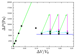
Figure 7: Black dots: inside-outside pressure difference $\Delta P$ for the first deflation of the ball of Fig. 5-b, versus its relative volume variation$\frac{\Delta V}{V_{0}}$. For points after the buckling ($\frac{\Delta V}{V_{0}}>0.05$), the pressure is calculated from the asymptotic value of $h\left(t\right)$ obtained through the biexponential fit such as in Fig. 5-b. Blue disks represent $\rho gh$ for measurements of $h\left(t\right)$ performed before stabilization of the water level in the manometer; this quantity, calculated out of equilibrium, does not correspond to the pressure difference through the ball, but its representation provides an estimation of the error performed if equilibrium is not attained. It is to be noted that the variation of water height in the manometer during the stabilization does not affect $\frac{\Delta V}{V_{0}}$ by a perceptible amount. In green and blue, respectively: the reconstructed linear part of the state equation (spherical deformation, Eq. (2)) up to the critical pressure difference (Eq. (3)), and the plateauing value of the post-buckling regime as proposed by heuristic Eq. (13). Arrows are associated with the discussion at the end of subsection 3.2.2.

The situation is indeed more complex for some ”slow devices” (ball+manometer) where, in the post-buckling state, the equilibrium takes more than a few seconds to stabilize after the opening of valve $\mathcal{V}_{m}$. In that case, water outtake generates a steep withdrawal of the water level in the manometer, followed by a slower increase toward a limit value (via an exponential or bi-exponential relaxation versus time, as exposed in subsection 3.2.1). We observed experimentally that the slope of the steep withdrawal (light blue in fig. 7) never overtakes the slope of the linear part (which corresponds to pure constriction of the shell). We then assume that the sucking out of $\delta V_{i}$ first generates a (rapid) uniform constriction of the surface (on the figure: green arrows with the same inclination than the linear part of $\wp(\frac{\Delta V}{V_{0}})$), which has enough time to partly relax via a rolling of the rim that encircles the depression (pink arrows) before the ball is reconnected to the manometer. The relaxation of $h$ observed afterwards, then, corresponds to the end of the rim rolling toward the $\left(\Delta V_{i+1},\Delta P_{i+1}\right)$ equilibrium configuration, possibly slowed down further by other phenomena discussed in the following subsection.

A quantitative model for identifying the origin of the characteristic time(s) that are observed after connection to the manometer is proposed in the next subsection.

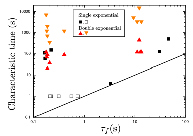
Figure 8: Characteristic equilibration times obtained from mono- or biexponential fit of experimental $h\left(t\right)$ curves, with respect to $\tau_{f}$, the time associated to viscous dissipation in the manometer, calculated using Eq. (8). Open squares: upper bound for the characteristic time of experiments leading to “immediate” equilibrium. Filled squares: unique characteristic time for shells showing a monoexponential decay during deflation. Upward red (resp. downward orange) triangles: short (resp. long) characteristic time for shells showing biexponential decay during deflation. The line indicates where the experimental times and $\tau_{f}$ (determined by Eq. (8)) would meet.

3.2.3 Relaxation towards equilibrium

As shown in figure 8, the characteristic time is around $2-500\,s$ for an exponential decay while when a biexponential fit is necessary, it unveils a longer characteristic time of $\approx 300-20000\,s$. Of course, for experiments where the water level stabilized ”immediately”, we only have an upper bound for the characteristic time(s), which is the few seconds that are necessary to operate the valves before measuring $h$.

When valve $\mathcal{V}_{m}$ is turned open after a deflation step, the water level in the manometer has to move in order to adapt to the new pressure. Assuming a Stokes incompressible flow in the vertical tube due to pressure difference $\Delta P$ between both extremities, this writes:

$$8\eta\left(L-h(t)\right)\frac{dh(t)}{dt}-r^{2}\Delta P(t)+r^{2}\rho gh(t)=0,$$ (6)

where $\eta$ is the viscosity of the water, $L$ the total length of the manometer, i.e. from the ball entry to the position of the meniscus at initial state. We neglected the section variations at the level of the valves and connections, and in the following we will replace $L-h$ by $L$ because $h\ll L$. Rewriting Eq. (6) then leads to:

$$\tau_{f}\frac{dh(t)}{dt}+h(t)=\frac{\Delta P(t)}{\rho g},$$ (7)

where $\tau_{f}$ is a caracteristic time for the decay of the water level toward its equilibrium value, and depends on experimental parameters through:

$$\tau_{f}=8\eta L/(\rho gr^{2}).$$ (8)

However, this fluid viscous dissipation is not the only possible contribution to the water level dynamics. As exposed in the end of the previous subsection, internal frictions in the material that forms the shell may be of importance. Our assessment is that, because of dissipation in the shell’s material, the pressure difference between both sides of the shell may evolve with a characteristic time $\tau_{s}$ toward the equilibrium situation where $\Delta P=\wp(\Delta V)$:

$$\tau_{s}\frac{\Delta P(t)}{dt}+\Delta P(t)=\wp(\Delta V(t)).$$ (9)

Here, we assume that $\tau_{s}$ is independent from the shape along the equilibration process in the manometer, which is reasonable as soon as small volume variations are imposed at each measurement step.

When opening valve $\mathcal{V}_{m}$ in order to measure the pressure, the system evolves from the intermediate state $(\Delta V_{i},$ $\Delta P_{i+1,interm})$ to the state $\left(\Delta V_{i+1},\Delta P_{i+1}\right)$; equations (9) and (7) together with the relationship $\Delta V=\Delta V_{i}+\delta V_{i}+\pi r^{2}(h_{i}-h)$ eventually lead to the evolution equation for $h$:

$$\tau_{f}\tau_{s}\frac{d^{2}h(t)}{dt^{2}}+(\tau_{f}+\tau_{s})\frac{dh(t)}{dt}+h(t)\\ =\frac{\wp(\Delta V_{i}+\delta V_{i}+\pi r^{2}(h_{i}-h(t)))}{\rho g}.$$ (10)

Before going further in the study of the dynamics towards measurable equilibrium states, let us focus on the latter, which we denote with stars. These states are characterized by hydrostatic relationship $\wp(\Delta V^{*})=\rho gh^{*}$, with:

$$\Delta V^{*}=\Delta V_{i}+\delta V_{i}+\pi r^{2}(h_{i}-h^{*}).$$ (11)

Because we explore the diagram step-by-step, the system is never far from its fixed point (except at the moment of exact buckling, that we do not consider here), so that we can expand the second term of equation (10) around it : $\wp(\Delta V)=\wp(\Delta V^{*})+\frac{d\wp}{d\Delta V}(\Delta V^{*})\times(\Delta V-\Delta V^{*})$, and eventually:

$$\tau_{f}\tau_{s}\frac{d^{2}h(t)}{dt^{2}}+(\tau_{f}+\tau_{s})\frac{dh(t)}{dt}\\ +\big{[}1+\frac{\pi r^{2}}{\rho g}\times\frac{d\wp}{d\Delta V}(\Delta V^{*})\big{]}(h(t)-h^{*})\\ =\frac{\wp(\Delta V^{*})}{\rho g}-h^{*}.$$ (12)

Initial conditions at $t=0$ are $h=h_{i}$, and from Eq (7), $\tau_{s}\frac{dh}{dt}=\frac{\Delta P}{\rho g}-h_{i}=\frac{\Delta P_{i+1,interm}}{\rho g}-h_{i}$, which depends on the moment at which the manometer was put in contact with the shell.

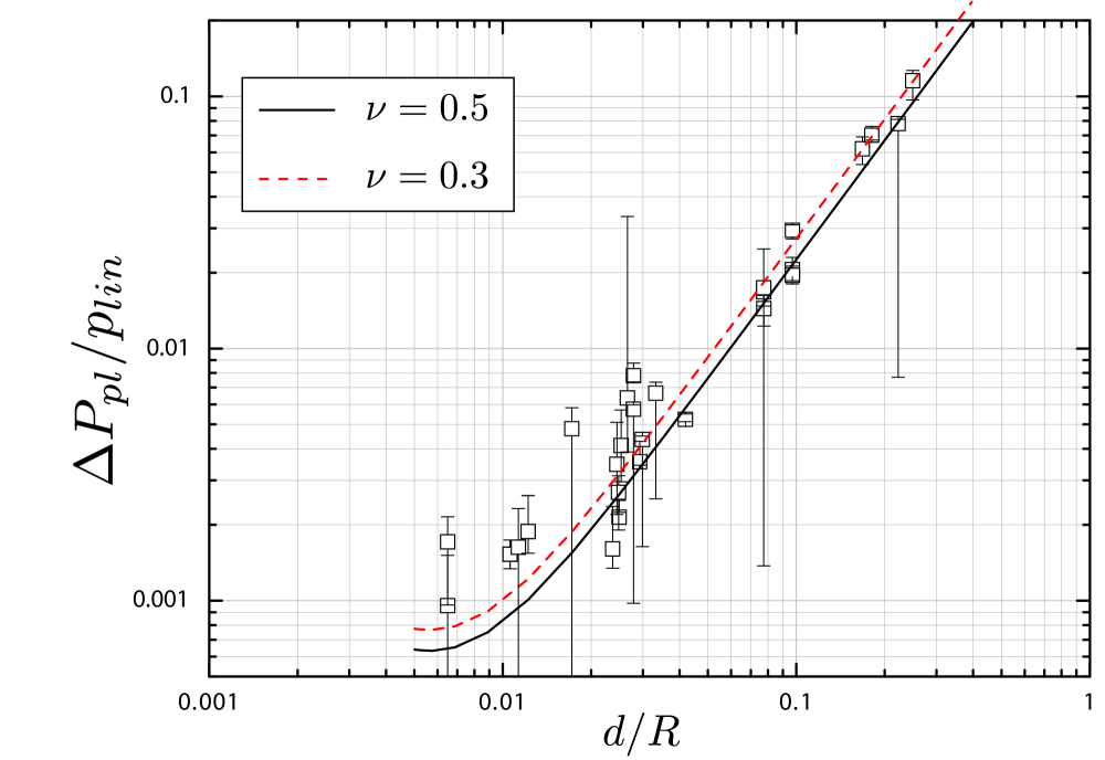
Figure 9: Squares: values of $\Delta P_{pl}/p_{lin}$, obtained from deflation curves similar to Fig. 4-b or Fig. 7, where $\Delta P_{pl}$ is the minimum value of the post-buckling regime, normalized by the slope $p_{lin}$ of the pre-buckling linear part. Lines: theoretical values determined using Eq. (14).

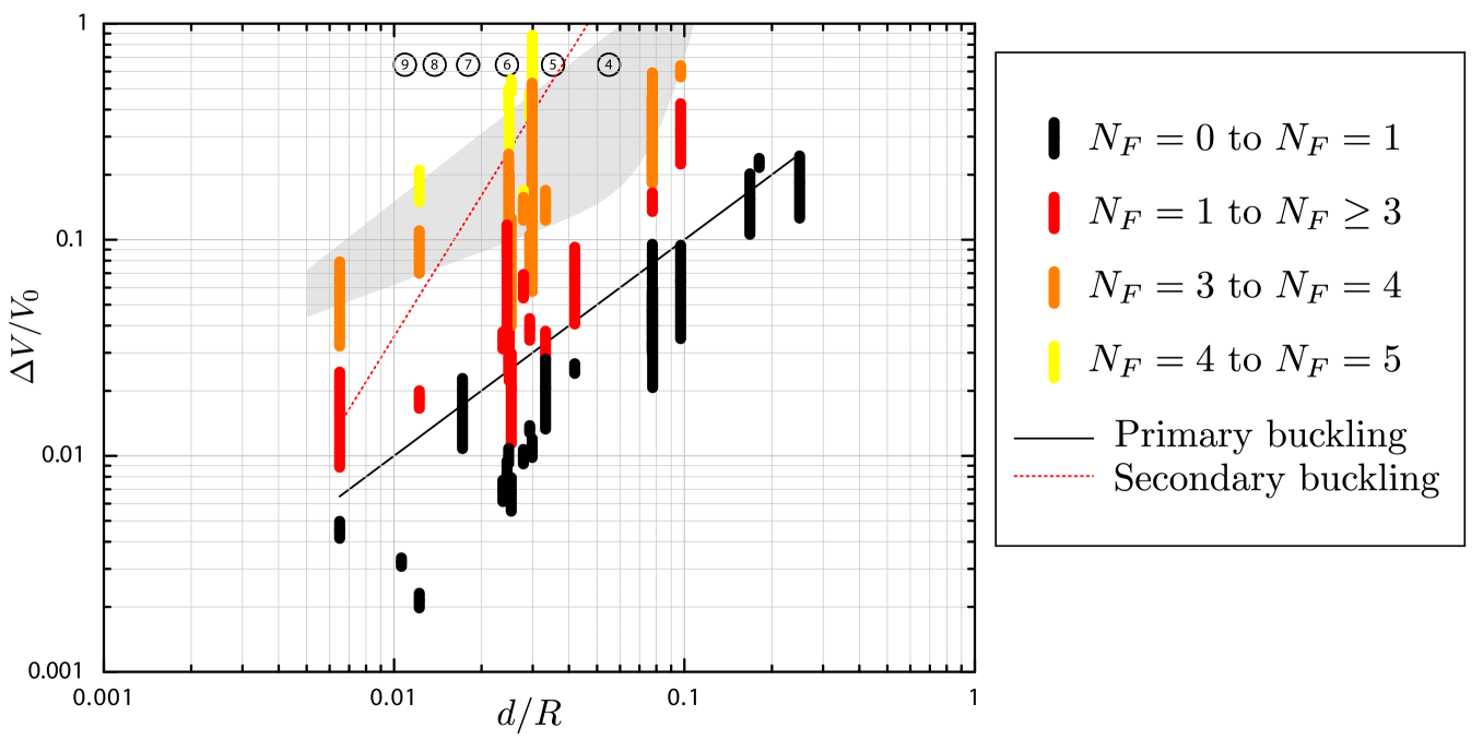
Figure 10: Shape diagram during deflation in the $(d/R,\Delta V/V_{0})$ space. Thick lines indicate the $\Delta V/V_{0}$ value range for which the considered transition was experimentally observed during deflation. Black: first buckling transition. Red: second buckling transition (from $N_{F}=1$ to $N_{F}\geq 3$). Orange: transition to $N_{F}=4$. Yellow: transition to $N_{F}=5$. The grey area is an indicator of the domain of existence of the $N_{F}=4$ configuration. Black thin line indicates the theoretical boundary for the primary transition for $\nu=0.5$ (see. Eq. 8 in Ref. Quilliet_2012 ). Red dashed line indicate the secondary transition as obtained from Eq. 11 in Quilliet_2012 with $\nu=0.5$. Theoretical boundaries depend only weakly on $\nu$. In the black circles are indicated the expected values for $N_{F}$ at the end of the plateau ($\Delta V/V_{0}\in[0.53;0.76]$), which are displayed in Fig. 11.

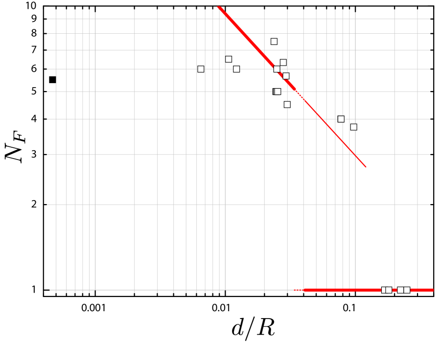
Figure 11: Number $N_{F}$ of folds, averaged for observations between $\Delta V/V_{0}=0.53$ and 0.76 (open squares). Full square is the experimental point of Ref. Carlson_1968 . $N_{F}=1$ stands for ”axisymmetric dimple”. The thick line indicates the expected $N_{F}=0.94\times(d/R)^{-1/2}$, obtained from the analysis of simulations in the same deflation range Quilliet_2012 . The dashed line corresponds to situations where the secondary buckling takes place in the $[0.53,0.76]$ range for $\Delta V/V_{0}$. The thin line corresponds to an extrapolation of the heuristic law in the $d/R$ range where simulations did not predict the secondary buckling.

One can easily show that the characteristic equation associated with the left part of Eq. 12 has two roots with negative real parts if $\left[\frac{d\wp}{d\Delta V}(\Delta V^{*})\right]>\left[-\frac{\rho g}{\pi r^{2}}\right]$. If this is not the case, the fixed point is not a stable point and cannot be reached, as already discussed in the geometrical construction of Fig. 6. This implies we cannot explore parts of the $\wp(\Delta V)$ state function where the slope is too strongly negative. Those are scarce in the diagram Knoche2011 , which justifies the choice of a U-shape manometer with water below the air at the level of the interface.

The strongest slopes are met in the isotropic phase. In that case, $\frac{d\wp}{d\Delta V}(\Delta V^{*})\sim Y_{3D}\times\frac{d}{R}\times\frac{1}{V_{0}}$. Considering $r=0.5$ mm, $Y_{3D}=7$ MPa, the highest value 0.25 for $d/R$ and the lowest value $40$ mm for the shell radius, we find that $\frac{\pi r^{2}}{\rho g}\times\frac{d\wp}{d\Delta V}(\Delta V^{*})$ never exceeds 0.5, so this term can be safely ignored in Eq. (12) when one studies post-buckling states.

For the isotropic phase as for the plateau, the solution of Eq. 12 is therefore a biexponential function with characteristic times $\tau_{f}$ and $\tau_{s}$.

The theoretical $\tau_{f}$, calculated using Eq. (8), was compared (Fig. 8) to the characteristic time(s) experimentally obtained, to which we incorporated data from the ”instantaneous” experiments by estimating the upper bond for the characteristic time as $1\,$s. We observe that apart from one case, the characteristic times are much higher than the viscous time $\tau_{f}$. This suggests that the times experimentally determined are intrinsic to the shells themselves, which are made of commercial polymers. Eq. 9 needs to be refined to account for this more complex relaxation scenario, which depends strongly on the ball under consideration as 0, 1 or 2 characteristic times larger than a few seconds can emerge. One may wonder why the viscous fluid characteristic time was not observed in more cases: the sampling was adapted to the slow relaxation dynamics of the shells, preventing data collection at times necessary to detect exponential contribution(s) with a characteristic time of a few seconds.

Finally, the choice of an intermediate section for the manometer enables us to obtain fluid dissipation times well-separated from that associated with the dissipation in the shell material, without hindering our ability to explore the state diagram by the use of too large sections.

3.2.4 Plateau values

We denominate by $\Delta P_{pl}$ (”plateau value”) the minimum value of the outside-inside pressure difference $\Delta P$, in the very flattened U-shaped part of the curve after buckling.

This quantity was previously studied through numerical simulations in Ref. Quilliet_2012 , and a heuristic dependance had been found between $\Delta P_{pl}$ and $\frac{\Delta V}{V_{0}}$. For the present paper, we extended the simulations range and we use a different formula to fit the simulations for the whole range of experimental $\frac{d}{R}$, i.e. from $5.10^{-3}$ to 0.3:

$$\Delta P_{pl}=\frac{Y_{3D}}{\left(1-\nu^{2}\right)^{0.75}}\times\left(2.34\,10^{-6}+0.9\left(d/R\right)^{2.57}\right)$$ (13)

In order to check the consistency of the deflation experiments with the theory, we determined for each ball the slope $p_{lin}$ of the linear part. Theoretically, $p_{lin}=\frac{2Y_{3D}}{3\left(1-\nu\right)}\times\frac{d}{R}$ (from Eq. (2)). We then focussed on the nondimensionalized value $\frac{\Delta P_{pl}}{p_{lin}}$ (which avoids concerns about an independent determination of $Y_{3D}$) with respect to $\frac{d}{R}$, as displayed in Fig. 9. It shows that these experimental points are consistent with the theoretical curve obtained from Eq. (13) and the expression of $p_{lin}$:

$$\frac{\Delta P_{pl}}{p_{lin}}=\frac{\left(1-\nu\right)^{0.25}}{\left(1+\nu\right)^{0.75}}\left[3.51\,10^{-6}+1.35\left(\frac{d}{R}\right)^{2.57}\right]\left(\frac{d}{R}\right)^{-1}$$ (14)

This result is new and of practical interest, since equation (13) had been established for thin shells. The experiments presented here show its validity for shells with relative thickness up to $\frac{d}{R}\approx 0.3$.

3.2.5 Towards folding

As the ball deflates along the postbuckling plateau, folds appear in the depression for the thinnest of the shells, as in Fig. 2-b. This secondary buckling transition is documented in literature for thin shells, both experimentally Carlson_1968 for very thin shells and theoretically Knoche2014 ; Hutchinson_2017 , but the only results for what concerns shells of medium thickness ($d/R>0.02$) were obtained numerically Quilliet2008 ; Quilliet_2012 . Experimental domains of existence of emblematic non axisymmetric conformation are represented in Fig. 10 in the $(d/R,\Delta V/V_{0})$ space. They show some discrepancies with the boundaries obtained from simulations Quilliet2008 ; Quilliet_2012 .

Primary buckling occurred for a volume loss much lower than that predicted in simulations ; as in Sec. 3.1, defects are expected to be the cause of this discrepancy.

The secondary buckling towards non-axisymmetric shapes also occurred for values of the relative deflation significantly lower than in simulations. Such shapes present radial folds, the number of which is denominated by $N_{F}$. In our experiments, the transition out from an axisymmetric shape could happen by way of an elongation of the dimple (the shape is then characterized by $N_{F}=2$, as in Ref. Carlson_1968 ) and could be continued by the development of three fold shape ($N_{F}=3$). Both types of shapes were not obtained in the simulations of Ref. Quilliet_2012 . In these simulations, $N_{F}=4$ was seldom observed while the $N_{F}=4$ zone shows a great extent in the experimental diagram of Fig. 10. Finally, the experimental domain of transition from $N_{F}=3$ to $N_{F}=4$ is crossed by the heuristic transition line found in Ref. Quilliet_2012 for the secondary buckling, that is characterized by a $N_{F}=1$ to $N_{F}\geq 4$ direct transition. It may indicate that, for some numerical reason, the energy minima corresponding to low numbers of folds were not found by the solver in the simulations, that were then stuck to axisymmetric shapes. Note that the secondary buckling transition line found by Knoche and Kierfeld in Ref. Knoche2014 is close to that proposed in Ref. Quilliet_2012 , that serves here as a reference for this discussion.

Notwithstanding this discrepancy in the boundaries of the axisymmetric zone, we aim here at checking the heuristic dependence with $d/R$ of the number of folds $N_{F}$ reached at the end of the plateau, proposed in Ref. Quilliet_2012 .

For the thinnest of the shells, the number of folds clearly departs from this heuristic law, as shown in Fig. 11. This discrepancy may be due to the intrinsic limitations of an elastic model, failing to describe microscopic phenomena at stake at the apex of the s-cones in thin shells, where sharp creases are likely to host plastic deformation Nasto2013 . Interestingly, for thick enough shells ($d/R>0.01$) less prone to extreme deformations, the number of folds roughly follows the proposed law in $(d/R)^{-1/2}$, thus confirming the relevance of $\sqrt{dR}$ as the key length for the elastic deformations of shells Quilliet_2012 .

4 Comparison with traction experiments

Elastic properties (Young modulus and Poisson’s ratio) were directly measured with a tensile tester Shimadzu Autograph AGS-X machine equipped with a 100 N load cell. The tensile tests were performed at ambient temperature on dumbbell-shaped sample cut with a dogbone punch (gauge length$18$ mm $\times 4$ mm) in the ball, hence presenting a thickness $d$. Traction was performed at a maximum crosshead speed of 2 mm/min. For each ball, two different samples were submitted to two tractions at a maximum deformation of 3%, during which force and elongations (both longitudinal and transversal, using instant image treatment) were recorded. The true stress was plotted as a function of the nominal strain, and the Young’s modulus was determined from the initial slope of the stress/strain curves. Video recording of the sample during the deformation was performed in order to measure the Poisson’s ratio. Non-linearity between longitudinal and transversal deformations prevented reliable measurement of $\nu$ for half of the samples. When we were able to unambiguously determine its values, we found $0.45\leq\nu\leq 0.5$, as is typical for elastomeric materials. Regardless, the Poisson’s ratio has a small effect on values of interest, as shown by theoretical curves of figures 9 and 12. Figure 12 shows that there is a satisfactory agreement for most of the shells between the slope $p_{lin}$ of the $\wp(\Delta V)$ equilibrium diagram in the isotropic deflation regime, adimensionalised by $Y_{3D}$ measured by traction experiments, and its theoretical value computed from $d/R$ and $\nu$. We recall that most of the studied shells are low-cost toys obtained by rotational casting with some variations of the thickness along the surface. These results indicates that for moderate deformations, in-plane compression (that operates in deflation experiments) and traction can be described using the same linear Young modulus.

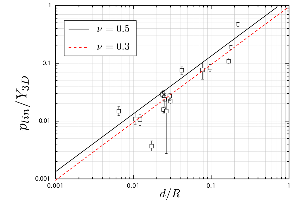
Figure 12: Slope $p_{lin}$ of the linear part of the $\Delta P\left(\frac{\Delta V}{V_{0}}\right)$ diagram, adimensionnalized by the Young modulus $Y_{3D}$ directly measured from traction experiments. Straight lines : theoretical curves for $p_{lin}/Y_{3D}=\frac{2}{3\left(1-\nu\right)}\times\frac{d}{R}$, displayed for two values typically bounding the Poisson’s ratio of the shells studied.

5 Conclusion and discussion

Through theoretical and/or numerical studies, previous literature provided hints about the behaviour of a ball that buckles under pressure, according to its relative volume change, relative thickness and Poisson’s ratio. This was mostly obtained through the use of a model of elastic surface whose range of validity is, a priori, restricted to thin shells ($d/R<0.02$). The experimental study conducted in this paper showed that thin shells deflate according to these models, with quantitative agreement for the relationships between volume and inside-outside pressure difference controlled by the Young modulus of the ball. More surprisingly, the agreement between the numerical deflation of elastic surfaces and the experimental results on shells of an isotropic material still holds for thicker shells (with important relative thicknesses, up to almost 0.3), when the correspondence between 3D features and the 2D properties of the model surface is kept unchanged.

We also identified the dynamics for the rolling of the rim (which encloses the depression formed during the buckling), with 1 or 2 relaxation characteristic times, depending on the properties that are associated to the dissipation in the material. We plan to run dynamical simulations in the future with models for shell membrane incorporating dissipation, so as to identify the source of these different times.

These results bring essential clues to the deflation of shells, and quantitative insights in a range of parameters that has not yet been explored experimentally or theoretically.

6 Acknowledgements

We thank Pierre Saillé (CERMAV) for introducing us to traction experiments, and Guillaume Laurent and Antonin Borgnon for their involvement as students in the first experiments. A.D.’s position was funded by the European Research Council under the European Union s Seventh Framework Programme (FP7/2007 2013)/ERC Grant No. 614655 Bubbleboost.

7 Authors contributions

G.C. and C.Q. have designed the research and the experimental set-up. All the authors carried out the experiments. C.Q. has realised the additional numerical simulations. G.C. and C.Q. were involved in the preparation of the manuscript. All the authors have read and approved the final manuscript.

References

- (1) J. W. Hutchinson, J. Appl. Mech. 34, 49 (1967).
- (2) L. Landau, E. M. Lifschitz, Theory of elasticity, 3rd ed., Elsevier Butterworth-Heinemann, Oxford (1986).
- (3) C. Quilliet, C. Zoldesi, C. Riera, A. van Blaaderen, A. Imhof, Eur. Phys. J. E 27, 13 (2008).
- (4) C. Quilliet, C. Zoldesi, C. Riera, A. van Blaaderen, A. Imhof, Eur. Phys. J. E 32, 419 (2010).
- (5) S. Knoche and J. Kierfeld, Phys. Rev. E 84, 046608 (2011).
- (6) G. A. Vliegenthart, G. Gompper, New J. Phys. 13, 045020 (2011).
- (7) C. Quilliet, Eur. Phys. J. E 35, 48 (2012).
- (8) J. W. Hutchinson, J. M. T. Thompson, Phil. Trans. R. Soc. A 375, 20160154 (2017).
- (9) M. Pezzulla, N. Stoop, M.P. Steranka, A.J. Bade, and D.P. Holmes, Phys. Rev. Lett. 120, 048002, (2018).
- (10) R. L. Carlson, R. L. Sendelbeck, N. J. Hoff, Exp. Mech. 7, 281 (1967).
- (11) L. Berke, R. L. Carlson, Exp. Mech. 8, 548 (1968).
- (12) J. Zhang, M. Zhang, W. Tang, W. Wang, M. Wang, Thin-Walled Str. 111, 58 (2017).
- (13) S. Knoche, J. Kierfeld, Eur. Phys. J. E 37, 62 (2014).
- (14) C. C. Church, J. Acoust. Soc. Am. 97, 1510 (1994).
- (15) A. Djellouli, P. Marmottant, H. Djeridi, C. Quilliet, G. Coupier, Phys. Rev. Lett. 119, 224501 (2017).
- (16) Y. Forterre, J. M. Skotheim, J. Dumais, L. Mahadevan, Nat. 433, 421 (2005).
- (17) O. Vincent, C. Weisskopf, S. Poppinga, T. Masselter, T. Speck, M. Joyeux, C. Quilliet, P. Marmottant, Proc. Roy. Soc. B: Biol. Sci. 278, 2909 (2011).
- (18) K. Son, J. S. Guasto, R. Stocker, Nat. Phys. 9, 494 (2013).
- (19) D. P. Holmes, A. J. Crosby, Adv. Mater. 19, 3589, (2007).
- (20) D. Yang, B. Mosadegh, A. Ainla, B. Lee, F. Khashai, Z. Suo, K. Bertoldi, G. M. Whitesides, Adv. Mater. 27 6323 (2015).
- (21) V. Ramachandran, M. D. Bartlett, J. Wissman, C. Majidi, Extreme Mech. Lett. 9, 282 (2016).
- (22) M. Gomez, D. E. Moulton, D. Vella, Phys. Rev. Lett. 119, 144502 (2017).
- (23) D. P. Holmes, Curr. Op. Coll. Interf. Science 40, 118 - 137 (2019).
- (24) A. V. Pogorelov, Bending of surfaces and stability of shells (American Mathematical Society, Providence, 1988).
- (25) J. W. Hutchinson, Proc. Roy. Soc. A 472, 20160577 (2016).
- (26) F. Quéméneur, C. Quilliet, M. Faivre, A. Viallat, B. Pépin-Donat, Phys. Rev. Lett. 108, 108303 (2012).
- (27) P. Marmottant, A. Bouakaz, N. De Jong, C. Quilliet, J. Acoust. Soc. Am. 129, 1231 (2011).
- (28) D. Vella, A. Ajdari, A. Vaziri, A. Boudaoud, Phys. Rev. Lett. 107, 174301 (2011).
- (29) J. Marthelot, F. López Jiménez, A. Lee, J. Hutchinson, P.M. Reis, J. Appl. Mech. 84, 121005 (2017).
- (30) A.Nasto, A. Ajdari, A. Lazarus, P. Reis, Soft Matt. 9, 6796 (2013).