Abstract

In this paper, a parameter-uniform fitted mesh finite difference scheme is constructed and analyzed for a class of singularly perturbed interior turning point problems. The solution of this class of turning point problem possess two outflow exponential boundary layers. Parameter-explicit theoretical bounds on the derivatives of the analytical solution are given, which are used in the error analysis of the proposed scheme. The problem is discretized by a hybrid finite difference scheme comprises of midpoint-upwind and central difference operator on an appropriate piecewise-uniform fitted mesh. An error analysis has been carried out for the proposed scheme by splitting the solution into regular and singular components and the method has been shown second order uniform convergent except for a logarithmic factor with respect to the singular perturbation parameter. Some relevant numerical examples are also illustrated to verify computationally the theoretical aspects. Numerical experiments show that the proposed method gives competitive results in comparison to those of other methods exist in the literature.

Keywords: singularly perturbed turning point problem; boundary layer; finite difference; fitted mesh; error estimates

1 Introduction

Singularly perturbed problems arise often in the modeling of various modern complicated processes, such as viscous flow problems with large Reynolds numbers [9], convective heat transport problems with large Péclet numbers [10], drift diffusion equation of semiconductor device modelling [21], electromagnetic field problems in moving media [8], financial modelling [5] and turbulence models [15] etc. Most of the singularly perturbed problems cannot be completely solved by analytical techniques. Consequently, numerical techniques are getting much attention to get some useful insights on the solutions of singularly perturbed problems. In general, two classes of methods, namely, fitted operator methods and fitted mesh methods have been used to solve such problems.

Those singularly perturbed convection-diffusion problems, in which the convection coefficient vanishes at some points of the domain of the problem, are called singularly perturbed turning point problems (SPTPPs), and zeros of the convection coefficient are said to be turning points. Here, we consider the following class of singularly perturbed two-point boundary value problems with an interior turning point at $x=0$ [12]:

$$\begin{cases}\mathcal{L}u(x)\equiv\varepsilon u^{\prime\prime}(x)+a(x)u^{\prime}(x)-b(x)u(x)=f(x),\qquad x\in\Omega=(-1,1),\\ u(-1)=A,\qquad u(1)=B,\end{cases}$$ (1.1)

where $\varepsilon$ is a small perturbation parameter satisfying $0<\varepsilon<<1$, $A$ and $B$ are given constants, $a,b$ and $f$ are sufficiently smooth functions. We impose the following restriction to ensure that the solution of Eq. (1.1) exhibits twin boundary layers

$$a(0)=0,\qquad a^{\prime}(0)<0.$$ (1.2)

Moreover, for some constant $\delta>0$ there exists a positive constant $\alpha$, such that

$$|a(x)|\geq\alpha>0,\qquad\delta\leq|x|\leq 1.$$ (1.3)

Also $b(x)$ is required to be bounded below by some positive constant $\beta$, $i.e.$,

$$b(x)\geq\beta>0,\qquad x\in\bar{\Omega}=[-1,1],$$ (1.4)

to guarantee that the operator $\mathcal{L}$ is inverse monotone on $[-1,1]$ and to exclude the so-called resonance phenomena [2]. We also impose the following restriction to ensure that there are no other turning points in the interval $[-1,1]$:

$$|a^{\prime}(x)|\geq\left|\frac{a^{\prime}(0)}{2}\right|,\qquad x\in\bar{\Omega}=[-1,1].$$ (1.5)

This class of singularly perturbed turning point problem (SPTPP)  (1.1) has a unique solution possess twin outflow boundary layers of exponential type at both end points $x=\pm 1$, under the assumptions  (1.2)- (1.5).

It is very difficult to deal singularly perturbed turning point problems analytically. The study of these problems received much attention in the literature due to the complexity involved in finding uniformly valid asymptotic expansions unlike non-turning problems. Some authors, such as, Jingde [7], O’Malley [16, 17], Wasow [24] studied qualitative aspects of these problems, namely, existence, uniqueness and asymptotic behavior of the solution.

In general, since the convection coefficient has zero inside the domain therefore numerical treatment of singularly perturbed turning point problem becomes more difficult than the singularly perturbed non-turning point problems. Abrahamsson [1], Berger et al. [3] and Farrell [6] establish a priori bounds for interior turning point problems; in particular it is shown that a bound is independent of singular perturbation parameter $\varepsilon$ if and only if reaction coefficient is greater than zero at the turning point. It is also shown there how the ratio of reaction coefficient $b(x)\geq 0$ and first derivative of convection coefficient $a^{\prime}(x)$, $i.e.$, $\lambda=b(x)/a^{\prime}(x)$ at the turning point plays a key role in determining the behavior of the solution [3]. It is shown that for $\lambda<0$, the solution is smooth near turning point and two outflow boundary layers of exponential type exhibits at both the endpoints of the domain. In this case the turning point is sometimes called a diverging flow or expansion turning point. On the other hand, if $\lambda>0$, there is in general no boundary layers exhibited and an interior layer appears at the turning point, the nature of which depends in a fundamental way on $\lambda$. For $0<\lambda<1$, the interior layer is called cusp layer because it can be approximately modelled by a cusp-like function. Interior layer turning point is sometimes called a converging flow or compression turning point. In inviscid fluid dynamics, the diverging flow turning point corresponds to a sonic point and converging flow turning point to a shock point. For the case $b(x)=0$ at the turning point, the solution exhibits a very interesting phenomenon called Ackerberg-O’Malley resonance phenomenon [2].

Berger et al. [3] also show that the modified version of El Mistikawy Werle scheme is uniformly convergent of $O(h^{\min(\lambda,1)})$ in the $L^{\infty}[-1,\,1]$ norm using the analytic bounds obtained in [3]. Farrell [6] obtained a set of sufficient conditions for uniform convergence in the discrete $L^{\infty}$ norm on uniform mesh, not only for exponentially fitted schemes, but also for a large class of schemes of upwinded type. Kadalbajoo and Patidar [11] gave a numerical scheme based on cubic spline approximation with nonuniform mesh for SPTPP (1.1)-(1.5) and established second order $\varepsilon$-uniform convergence. Natesan et al. [20] proposed a numerical method based on the classical upwind finite difference scheme on a Shishkin mesh and proved that the proposed scheme is uniformly convergent of almost order one. In [12], Kadalbajoo and Gupta derived asymptotic bounds for the derivatives of the analytical solution of SPTPP (1.1)-(1.5) and proposed a computational method comprises B-spline collocation scheme on a non-uniform Shiskin mesh. They shown that this scheme is second order accurate in the maximum norm. Kadalbajoo et al. [13] also suggested B-spline collocation with artificial viscosity on uniform mesh for the same class of SPTPP (1.1)-(1.5). In [18], Munyakazi and Patidar conclude that convergence acceleration Richardson extrapolation technique on existing numerical schemes for the above class of turning point problem does not improve the rate of convergence. However, Becher and Roos [4] show that Richardson extrapolation on upwind scheme with piecewise-uniform Shishkin mesh works fine and improves the accuracy to $O(N^{-2}\ln^{2}N)$ under the assumption $\varepsilon\leq CN^{-1}$. Recently, Munyakazi et al. [19] proposed a fitted operator finite difference scheme for singularly perturbed turning point problem having an interior layer and also shown that with Richardson extrapolation technique, accuracy and order of convergence of the scheme can be improved upto two. For a general review of existing literature on asymptotic and numerical analysis of turning point problems, one can see [22].

In this paper, we focus to devise a second order uniformly convergent finite difference scheme for SPTPP (1.1) on piecewise uniform mesh of Shishkin type without using any convergence acceleration technique like Richardson extrapolation. The proposed method combines the midpoint upwind difference scheme and classical central finite difference scheme on piecewise uniform mesh. The requirements of higher order truncation error and monotonicity play a vital role in the construction of this scheme. One can observe the fact that the classical central difference scheme is monotone if $\varepsilon$ is relatively large than the convection coefficient $a$ $i.e.$, if $\varepsilon\geq Ch||a||$, where $h$ is the mesh width and has second order truncation error on uniform mesh. On the other hand, midpoint upwind difference operator is monotone for all value of $\varepsilon$ and for relatively large convection coefficient $a$ than the reaction coefficient $b$ such that $h||b||\leq C\alpha$. Moreover, midpoint upwind operator possess second order truncation error away from the boundary layer region. Also, Shiskin mesh equally distribute the number of mesh points inside and outside the boundary layers, therefore one can gets a coarse mesh region outside the boundary layer and fine mesh region inside the boundary layer. Utilizing these facts, we employ midpoint upwind difference scheme in coarse mesh region and central difference operator in fine mesh region of Shishkin mesh. Since, central difference operator yields first order truncation error at transition points, we use midpoint upwind operator on transition points. Such type of higher order scheme for singularly perturbed non-turning convection-diffusion problem was introduced by Stynes and Roos [23]. To analyze the proposed scheme theoretically, we split the numerical solution into regular and singular components and analyze them separately by using tools such as truncation error bounds, discrete minimum principle and appropriate choices of barrier functions.
Notation. Throughout the paper we use $C$ as a generic positive constant independent of $\varepsilon$ and mesh parameters. For any given function $g(x)\in C^{k}(\bar{\Omega})$ ($k$ a non-negative integer), $||g||$ is a global maximum norm over the domain $\bar{\Omega}$ defined by

$$||g||=\max_{\bar{\Omega}}|g(x)|.$$

2 A-priori Estimates for Continuous Problem

In this section some bounds of the exact solution and its derivatives are discussed. These bounds will be needed for error analysis of proposed numerical scheme in later sections. Derivation of these bounds are well known and can be found in [12]. Systematically, we use minimum principle to derive these bounds.

Lemma 2.1.

([12].) (Minimum Principle) Let $\psi(x)\in C^{2}(\bar{\Omega})$ and $\psi(\pm 1)\geq 0$. Then $\mathcal{L}\psi(x)\leq 0,\forall x\in\Omega$ implies that $\psi(x)\geq 0,\forall x\in\bar{\Omega}.$

Since the concerned SPTPP (1.1)-(1.5) is linear, minimum principle ensure the existence and uniqueness of the classical solution. Using the above minimum principle, one can easily prove the following uniform stability estimate for the differential operator $\mathcal{L}$.

Lemma 2.2.

([12].) (Uniform Stability Estimate) $\forall\varepsilon>0$, solution $u(x)$ of the SPTPP (1.1)-(1.5), satisfies the following stability estimate:

$$||u(x)||\leq\frac{||f||}{\beta}+\max(|A|,|B|),\qquad\forall x\in\bar{\Omega}.$$

To exclude the turning point $x=0$ and to obtain the bounds for the solution $u$ and its derivatives in the non-turning point region of the domain, we divide the domain $\bar{\Omega}$ into three subdomains as $\Omega_{1}=[-1,-\delta]$, $\Omega_{2}=[-\delta,\delta]$ and $\Omega_{3}=[\delta,1]$ such that $\bar{\Omega}=\Omega_{1}\cup\Omega_{2}\cup\Omega_{3}$, where $0<\delta\leq 1/2$. Further, following theorem gives bounds for the derivatives of $u$ in the subintervals $\Omega_{1}$ and $\Omega_{3}$ individually.

Theorem 2.1.

([12].) If $a,\,b$ and $f$ $\in C^{m}(\bar{\Omega}),m>0$, then solution $u(x)$ of the SPTPP (1.1)-(1.2) satisfies the following bounds for any $\delta>0$:

$$|u^{j}(x)|\leq C\left(1+\varepsilon^{-j}\exp\left(-\frac{\alpha(1+x)}{\varepsilon}\right)\right),\quad j=1,\cdots,m+1,\quad x\in\Omega_{1},$$

$$|u^{j}(x)|\leq C\left(1+\varepsilon^{-j}\exp\left(-\frac{\alpha(1-x)}{\varepsilon}\right)\right),\quad j=1,\cdots,m+1,\quad x\in\Omega_{3},$$

Next, we state a theorem, which gives the bounds for the derivatives of the solution in the turning point region $\Omega_{2}$ and deduce that the solution is smooth in subdomain $\Omega_{2}$.

Theorem 2.2.

([3].) Let $u(x)$ be the solution of SPTPP defined from the equations(1.1)-(1.5), and $a,\,b,\,f\in C^{m}(\bar{\Omega}),m>0$. Then for $\varepsilon>0$ and sufficiently small $\delta>0$, there exists a positive constant $C$ such that

$$|u^{(j)}(x)|\leq C,\quad j=1,2,\ldots,m,\quad\forall x\in\Omega_{2}.$$

It turns out that the bounds for continuous solution $u(x)$ given in Theorem 2.1 and Theorem 2.2 are not adequate to obtain $\varepsilon$-uniform error estimate for the proposed scheme. Therefore, to analyze the proposed scheme correctly, we need to derive more precise bounds on these derivatives by decomposing the solution into regular component $v$ and singular component $w$ as

$$u(x)=v(x)+w(x),\qquad\forall x\in\bar{\Omega},$$

where the smooth component $v$ satisfies homogeneous problem $\mathcal{L}v(x)=f(x)$ and singular component satisfies homogeneous problem $\mathcal{L}w(x)=0$ with appropriate boundary conditions. Using the technique given in [12], we get the following bounds for smooth and singular components in the region $\Omega_{1}$:

$$|v^{(j)}(x)|\leq C(1+\varepsilon^{((m-1)-j)}e^{-\alpha(1+x)/\varepsilon}),\qquad\forall x\in\Omega_{1},$$

$$|w^{(j)}(x)|\leq C\varepsilon^{-j}e^{-\alpha(1+x)/\varepsilon}.\qquad\qquad\qquad\forall x\in\Omega_{1}.$$

In the same manner, we can obtain analogous estimates for subinterval $\Omega_{3}$, while the solution $u(x)$ and its derivatives are smooth in the subinterval $\Omega_{2}$. Hence, on the whole domain $\bar{\Omega}$, the bounds on $v$ and $w$, and their derivatives are given in the following theorem:

Theorem 2.3.

([12].) Let $a,b$ and $f\in C^{m}(\bar{\Omega}),m>0,$ then for all $j,~{}0\leq j\leq m,$ the smooth component satisfies

$$|v^{(j)}(x)|\leq C\left(1+\varepsilon^{((m-1)-j)}\left(\exp\left(-\frac{\alpha(1+x)}{\varepsilon}\right)+\exp\left(-\frac{\alpha(1-x)}{\varepsilon}\right)\right)\right),\quad\forall x\in\bar{\Omega},$$

and the singular component satisfies

$$|w^{(i)}(x)|\leq C\varepsilon^{-i}\left(\exp\left(-\frac{\alpha(1+x)}{\varepsilon}\right)+\exp\left(-\frac{\alpha(1-x)}{\varepsilon}\right)\right),\quad\forall x\in\bar{\Omega}.$$

3 Fitted Mesh Higher-Order Scheme

In this section, first we construct fitted piecewise-uniform mesh $\bar{\Omega}^{N}$ of Shishkin type to discretize the domain $\bar{\Omega}$ and then employ a specially designed finite difference scheme on this mesh to discretize the SPTPP (1.1)-(1.2). The fitted mesh $\bar{\Omega}^{N}$ is constructed by dividing $\bar{\Omega}$ into three subintervals $\Omega_{L}=[-1,-1+\tau],\Omega_{C}=[-1+\tau,1-\tau]$ and $\Omega_{R}=[1-\tau,1]$ such that $\bar{\Omega}=\Omega_{L}\cup\Omega_{C}\cup\Omega_{R}$. For $N\geq 2^{r},\,r\geq 3$ be an integer, $\bar{\Omega}^{N}$ divides each of the subintervals $\Omega_{L}$ and $\Omega_{R}$ into $N/4$ mesh intervals and $\Omega_{C}$ with $N/2$ mesh intervals such that $\bar{\Omega}^{N}=\{-1=x_{0},\,x_{1},\ldots,x_{N/4}=-1+\tau,\ldots x_{3N/4}=1-\tau,\ldots,x_{N}=1\}$. Here, the transition parameter is obtained by taking

$$\tau=\min\left\{\frac{1}{4},\tau_{0}\varepsilon\ln N\right\}.$$

The constant $\tau_{0}$ is independent of the parameter $\varepsilon$ and the number of mesh points $N$ and will be chosen later on during the analysis of proposed scheme. This mesh is coarse on $\Omega_{C}$ and fine on $\Omega_{L}$ and on $\Omega_{R}$. If $h$ and $H$ are fine and coarse mesh width respectively, then mesh width $h_{i}=x_{i}-x_{i-1},\,i=1,\ldots,N,$ is defined as

$$h_{i}=\begin{cases}h=4\tau/N,&\text{ $i=1,2,\ldots,N/4$},\\ H=4(1-\tau)/N,&\text{ $i=N/4+1,\ldots,3N/4$},\\ h=4\tau/N,&\text{ $i=3N/4+1,\ldots,N$.}\end{cases}$$

One can easily observe that

$$N^{-1}\leq H\leq 4N^{-1},\quad h=4\tau_{0}\varepsilon N^{-1}\ln N<N^{-1},\quad H+h=4N^{-1}.$$

Since, convection coefficient $a(x)$ changes its sign at the turning point $x=0$, therefore, we construct a finite difference scheme $\mathcal{L}^{N}U_{i}=\tilde{f_{i}},\,i=1,2,\ldots,N-1$ to discretize the SPTPP (1.1) in the following manner

$$\mathcal{L}^{N}U(x_{i})\equiv\begin{cases}\mathcal{L}_{\text{c}}^{N}U\equiv\varepsilon\delta^{2}U_{i}+a_{i}D^{0}U_{i}-b_{i}U_{i}=f_{i},&i=1,2,\ldots,N/4-1,\\ \mathcal{L}_{\text{mp}}^{N}U\equiv\varepsilon\delta^{2}U_{i}+a_{i\pm 1/2}D^{\pm}U_{i}-(bU)_{i\pm 1/2}=f_{i\pm 1/2},&i=N/4,\ldots,3N/4,\\ \mathcal{L}_{\text{c}}^{N}U\equiv\varepsilon\delta^{2}U_{i}+a_{i}D^{0}U_{i}-b_{i}U_{i}=f_{i},&i=3N/4+1,\ldots,N-1,\\ U_{0}=A,\qquad U_{N}=B,\end{cases}$$ (3.1)

where,

$$\mathcal{L}_{\text{mp}}^{N}U\equiv\begin{cases}\varepsilon\delta^{2}U_{i}+a_{i+1/2}D^{+}U_{i}-(bU)_{i+1/2}=f_{i+1/2},&\text{if}~{}a_{i}>0\\ \varepsilon\delta^{2}U_{i}+a_{i-1/2}D^{-}U_{i}-(bU)_{i-1/2}=f_{i-1/2},&\text{if}~{}a_{i}<0.\end{cases}$$

Here, we used the following definition to construct above scheme

$$v_{i}=v(x_{i}),\quad v_{i+1/2}=\frac{v_{i}+v_{i+1}}{2},\quad v_{i-1/2}=\frac{v_{i-1}+v_{i}}{2},\quad\widehat{h}_{i}=\frac{h_{i}+h_{i+1}}{2},$$

$$D^{+}v_{i}=\frac{v_{i+1}-v_{i}}{h_{i+1}},~{},D^{-}v_{i}=\frac{v_{i}-v_{i-1}}{h_{i}},~{}D^{0}v_{i}=\frac{v_{i+1}-v_{i-1}}{2\widehat{h}_{i}},~{}\delta^{2}v_{i}=\frac{\left(D^{+}v_{i}-D^{-}v_{i}\right)}{\widehat{h}_{i}}.$$

It is clear that proposed finite difference operator $\mathcal{L}^{N}$ in scheme (3.1) is a combination of central difference operator $\mathcal{L}^{N}_{\text{c}}$ and midpoint upwind difference operator $\mathcal{L}^{N}_{\text{mp}}$, which is constructed by using knowledge judiciously about the sign of the convection term, location of the turning point and truncation error behavior of these operators. After simplifying the terms in (3.1), the difference scheme takes the form $\mathcal{L}^{N}U_{i}\equiv p_{i}^{l}U_{i-1}+p_{i}^{c}U_{i}+p_{i}^{r}U_{i+1}=\tilde{f_{i}}$, where the coefficients are given by

$$p_{i}^{l}=\left(\frac{\varepsilon}{h_{i}\widehat{h}_{i}}-\frac{a_{i}}{2\widehat{h}_{i}}\right),\qquad\qquad p_{i}^{c}=\left(-p_{i}^{l}-p_{i}^{r}-b_{i}\right),$$

$$p_{i}^{r}=\left(\frac{\varepsilon}{h_{i+1}\widehat{h}_{i}}+\frac{a_{i}}{2\widehat{h}_{i}}\right),~{}i=1,2,\ldots,N/4-1,~{}3N/4+1\ldots,N-1,$$

$$p_{i}^{l}=\left(\frac{\varepsilon}{h_{i}\widehat{h}_{i}}\right),~{}p_{i}^{c}=\left(-p_{i}^{l}-p_{i}^{r}-b_{i+1/2}\right),~{}p_{i}^{r}=\left(\frac{\varepsilon}{h_{i+1}\widehat{h}_{i}}+\frac{a_{i+1/2}}{h_{i+1}}-\frac{b_{i+1}}{2}\right),~{}\text{if}~{}a_{i}>0$$

$$p_{i}^{l}=\left(\frac{\varepsilon}{h_{i}\widehat{h}_{i}}-\frac{a_{i-1/2}}{h_{i}}-\frac{b_{i-1}}{2}\right),~{}p_{i}^{c}=\left(-p_{i}^{l}-p_{i}^{r}-b_{i-1/2}\right),~{}p_{i}^{r}=\left(\frac{\varepsilon}{h_{i+1}\widehat{h}_{i}}\right),~{}\text{if}~{}a_{i}<0,$$

$$i=N/4,\ldots,3N/4.$$

4 Uniform Convergence

Here, in this section first we shall establish the consistency and stability estimate through discrete minimum principle and then analyze proposed numerical method (3.1) for $\varepsilon$-uniform convergence by analogous decomposition of discrete solution into smooth and singular components as of continuous solution.

Lemma 4.1.

( Discrete Minimum Principle) Let us suppose that $N\geq N_{0}$, where

$$\frac{h||a||}{2\varepsilon}<1,~{}~{}i.e.,~{}~{}2\tau_{0}||a||<\frac{N_{0}}{\ln N_{0}},~{}~{}and~{}~{}\frac{2||b||}{N_{0}}\leq\alpha.$$ (4.1)

Then the operator $\mathcal{L}^{N}$ defined by (3.1) satisfies a discrete minimum principle, $i.e.,$ if $\psi^{N}$ is a mesh function that satisfies $\psi^{N}_{0}\geq 0,\,\psi^{N}_{N}\geq 0$ and $\mathcal{L^{N}}\psi_{i}^{N}\leq 0,$ for $1\leq i\leq N-1$, then $\psi_{i}^{N}\geq 0$ for $0\leq i\leq N$.

Proof. In order to establish the discrete minimum principle, We simply check that the associated system matrix is $M$-matrix with the choice of the midpoint upwind and central difference operator used in the definition of the difference scheme (3.1). It allow us to establish the following inequalities on the coefficients of the difference operator $\mathcal{L}^{N}$:

$$p_{i}^{l}>0,\qquad p_{i}^{r}>0,\qquad p_{i}^{l}+p_{i}^{c}+p_{i}^{r}<0,\qquad i=1,2,\ldots,N-1.$$ (4.2)

In the case of central difference operator $\mathcal{L}^{N}_{c}$, conditions in (4.2) are satisfied if $h||a||<2\varepsilon$ $i.e.,$ if $N_{0}(\ln N_{0})^{-1}>2\tau_{0}||a||$, then one can check $p_{i}^{l}>0$ and $p_{i}^{r}>0,\,p_{i}^{l}+p_{i}^{c}+p_{i}^{r}<0$ for $1\leq i\leq N/4-1$ and $3N/4+1\leq i\leq N-1$. For the case of midpoint upwind operator $\mathcal{L}^{N}_{\text{mp}}$, the conditions in (4.2) are satisfied if $H||b||<2\alpha$ $i.e.,$ if $2||b||<\alpha N_{0}.$ From these sign patterns on the coefficients of associated system matrix, one can deduce that operator $\mathcal{L}^{N}$ is of negative type and therefore satisfies a discrete minimum principle. Moreover, it ensures that the operator is uniformly stable in the maximum norm.

Lemma 4.2.

Let $Z^{N}_{i}$ be any mesh function such that $Z^{N}_{0}=Z^{N}_{N}=0.$ Then for all $i,\,0\leq i\leq N,$ we have

$$|Z^{N}_{i}|\leq\frac{1}{\beta}\max_{1\leq j\leq N-1}|\mathcal{L}^{N}Z^{N}_{j}|.$$

Proof. Let us introduce two comparison functions defined by

$$\Psi^{\pm}_{i}=\frac{1}{\beta}\max_{1\leq j\leq N-1}|\mathcal{L}^{N}Z^{N}_{j}|\pm Z^{N}_{i}.$$

Clearly one can notice that $\Psi^{N}_{0}=\Psi^{N}_{N}\geq 0,$ since $Z^{N}_{0}=Z^{N}_{N}=0.$ Furthermore, for $1\leq i\leq N-1,$ we have

$$\mathcal{L}^{N}\Psi^{\pm}_{i}=-\frac{b}{\beta}\max_{1\leq j\leq N-1}|\mathcal{L}^{N}Z^{N}_{j}|\pm\mathcal{L}^{N}Z_{i}^{N}\leq 0,$$

as $b/\beta\geq 1.$ Therefore, discrete minimum principle (4.1) implies that $\Psi^{\pm}_{i}\geq 0,\,0\leq i\leq N$, which gives desired result.

Further, using the valid Taylor’s series expansion, we obtained the following truncation error estimates for different finite difference operator employed in the operator $\mathcal{L}^{N}$: On a uniform mesh with step size $\tilde{h}$, we have

$$|\mathcal{L}_{\text{c}}^{N}u_{i}-(\mathcal{L}u)(x_{i})|\leq C(\varepsilon\tilde{h}^{2}|u^{(iv)}|+\tilde{h}^{2}|u^{(iii)}|).$$

On an arbitrary non-uniform mesh, we have

$$|\mathcal{L}_{\text{c}}^{N}u_{i}-(\mathcal{L}u)(x_{i})|\leq C\left(\varepsilon(h_{i}+h_{i+1})|u^{(iii)}|+(h_{i}+h_{i+1})|u^{(ii)}|\right).$$

Here, one can notice that order of truncation error is reduced to one only if the central difference operator is employed on arbitrary non-uniform mesh instead of uniform mesh. Moreover, We have the following truncation error bounds corresponding to the midpoint upwind difference operator, which are valid for both uniform and non-uniform mesh:

$$|\mathcal{L}_{\text{mp}}^{N}u_{i}-(\mathcal{L}u)(x_{i-1/2})|\leq\begin{cases}C\left(\varepsilon(h_{i}+h_{i+1})|u^{(iii)}|+h_{i+1}^{2}(|u^{(iii)}|+|u^{(ii)}|+|u^{i}|)\right),&\text{if}~{}a(x)>0,\\ C\left(\varepsilon(h_{i}+h_{i+1})|u^{(iii)}|+h_{i}^{2}(|u^{(iii)}|+|u^{(ii)}|+|u^{i}|)\right),&\text{if}~{}a(x)<0.\end{cases}$$

Note that the order of truncation error is higher by one in the convection term for midpoint upwind operator than the centered difference operator on a non-uniform mesh. This is the reason to apply midpoint upwind scheme at the transition points $(-1+\tau)$ and $(1-\tau)$ of proposed mesh.

Further the solution $U$ of the discrete problem can be decomposed in an analogous manner as that of the continuous solution $u$ into the following sum

$$U=V+W,$$ (4.3a)

where,

$$\mathcal{L}^{N}V=f,\quad V(-1)=v(-1),\,V(1)=v(1),$$ (4.3b)

$$\mathcal{L}^{N}W=0,\quad W(-1)=w(-1),\,W(1)=w(1).$$ (4.3c)

Therefore, the error can be written in the form

$$U-u=(V-v)+(W-w),$$

so the errors in the smooth and singular components of the solution can be estimated separately.

Lemma 4.3.

(Error in smooth component) Assume that $N\geq N_{0}$ satsifies the assumption (4.1). Then the regular component of the error satisfies the following error bound

$$|(V-v)(x_{i})|\leq\begin{cases}CN^{-2},\quad&\forall i=0,1,\ldots,N/4-1,3N/4+1,\ldots,N,\\ CN^{-1}(\varepsilon+N^{-1})&\forall i=N/4,N/4+1,\ldots,3N/4.\end{cases}$$

Proof. Using the usual truncation error estimates given above and bounds for the smooth component $v$ given in Theorem (2.3), we have

$$|\mathcal{L}^{N}(V-v)(x_{i})| \leq\begin{cases}CN^{-2}(\varepsilon|v^{(iv)}|+|v^{(iii)}|),\qquad\qquad\forall i=0,1,\ldots,N/4-1,3N/4+1,\ldots,N,\\ CN^{-1}(\varepsilon|v^{(iii)}|+N^{-1}(|v^{(iii)}|+|v^{(ii)}|+|v^{i}|)),\,\forall i=N/4,N/4+1,\ldots,3N/4.\\ \end{cases}$$

$$\leq\begin{cases}CN^{-2},\quad&\forall i=0,1,\ldots,N/4-1,3N/4+1,\ldots,N,\\ CN^{-1}(\varepsilon+N^{-1}),&\forall i=N/4,N/4+1,\ldots,3N/4,\end{cases}$$

and applying Lemma 4.2, we obtain the required result.

Since $a_{i}\geq\alpha>0,\,\forall x_{i}<0,\,i=1,\ldots,N/2$ and $a_{i}\leq-\alpha<0,\,\forall x_{i}>0,\,i=N/2+1,\ldots,N-1$, we consider both the region $[-1,0]$ and $[0,1]$ individually to get the error estimates for the layer component $(W-w)$. Therefore, we consider the following barrier functions for a positive constant $\gamma$:

$$\Phi_{i}^{L}=\begin{cases}\prod_{j=1}^{i}\left(1+\frac{\gamma h_{j}}{\varepsilon}\right)^{-1},\,&i=1,\ldots N/2,\\ 1,&i=0.\end{cases}\Phi_{i}^{R}=\begin{cases}\prod_{j=i+1}^{N}\left(1+\frac{\gamma h_{j}}{\varepsilon}\right)^{-1},\,&i=N/2,\ldots N-1,\\ 1,&i=N.\end{cases}$$ (4.4)

First we prove the following technical result.

Lemma 4.4.

If $2\gamma<\alpha$, the barrier functions satsisfy the inequalities

$$\mathcal{L}^{N}\Phi_{i}^{L}\leq 0,\quad\forall i=1,2,\ldots,N/2,\quad\mathcal{L}^{N}\Phi_{i}^{R}\leq 0,\quad\forall i=N/2,\ldots,N-1.$$

Proof. We begin with the left hand barrier function $\Phi_{i}^{L}$ and analyze each of the different discretizations used in the definition of the operator $\mathcal{L}^{N}$. First, in the case of midpoint upwind operator with $a(x)>0$, we have $\mathcal{L}^{N}\Phi_{i}^{L}=\mathcal{L}_{\text{mp}}^{N}\Phi_{i}^{L}=\varepsilon\delta^{2}\Phi_{i}^{L}+a_{i+1/2}D^{+}\Phi_{i}^{L}-(b\Phi^{L})_{i+1/2}$. Using the properties, $\Phi_{i}^{L}>0,$ $\,D^{+}\Phi_{i}^{L}=-\frac{\gamma}{\varepsilon}\Phi_{i+1}^{L}<0,$ and $\delta^{2}\Phi_{i}^{L}=\left(\frac{\gamma}{\varepsilon}\right)^{2}\frac{h_{i+1}}{\widehat{h}_{i}}\Phi_{i+1}^{L}>0$, and with the condition $2\gamma<\alpha$, one can easily observe that

$$\mathcal{L}_{\text{mp}}^{N}\Phi_{i}^{L} =\left(\frac{\gamma^{2}}{\varepsilon}\frac{h_{i+1}}{\widehat{h}_{i}}-a_{i+1/2}\frac{\gamma}{\varepsilon}-\frac{b_{i+1}}{2}\right)\Phi_{i+1}^{L}-\frac{b_{i}}{2}\Phi_{i}^{L}$$

$$=\left(2\frac{\gamma^{2}}{\varepsilon}\left(\frac{h_{i+1}}{2\widehat{h}_{i}}-1\right)+\left(2\frac{\gamma^{2}}{\varepsilon}-a_{i+1/2}\frac{\gamma}{\varepsilon}-\frac{b_{i+1}}{2}\right)-\frac{b_{i}}{2}\left(1+\frac{\gamma h_{i+1}}{\varepsilon}\right)\right)\Phi_{i+1}^{L}\leq 0.$$

In the case of central difference operator with $a(x)>0$, we have

$$\mathcal{L}_{\text{c}}^{N}\Phi_{i}^{L} =\left(2\frac{\gamma^{2}}{\varepsilon}\left(\frac{h_{i+1}}{2\widehat{h}_{i}}-1\right)+\left(2\frac{\gamma^{2}}{\varepsilon}-a_{i}\frac{\gamma}{\varepsilon}\frac{h_{i+1}}{2\widehat{h}_{i}}\right)\right)\Phi^{L}_{i+1}-\left(a_{i}\frac{\gamma}{\varepsilon}\frac{h_{i}}{2\widehat{h}_{i}}+b_{i}\right)\Phi_{i}^{L}\leq 0.$$

Similarly, applying the midpoint upwind operator for the case $a(x)<0$, we have

$$\mathcal{L}^{N}_{\text{mp}}\Phi_{i}^{R}=\left(2\frac{\gamma^{2}}{\varepsilon}\left(\frac{h_{i}}{2\widehat{h}_{i}}-1\right)+\left(2\frac{\gamma^{2}}{\varepsilon}+a_{i-1/2}\frac{\gamma}{\varepsilon}-\frac{b_{i-1}}{2}\right)-\frac{b_{i}}{2}\left(1+\frac{\gamma h_{i}}{\varepsilon}\right)\right)\Phi_{i-1}^{L}\leq 0.$$

In the same manner if we use central difference operator with $a(x)<0$, we also get $\mathcal{L}^{N}_{\text{c}}\Phi_{i}^{R}\leq 0.$ It completes the proof.

Lemma 4.5.

The barrier functions $\Phi_{i}^{L}$ and $\Phi_{i}^{R}$ and layer component $W$ satisfy

$$|W_{i}|\leq C\Phi_{i}^{L},\quad\forall i=0,1,\ldots N/2,\quad|W_{i}|\leq C\Phi^{R}_{i},\quad\forall i=N/2,\ldots,N.$$

Moreover, following bounds are valid for the layer component $W$ in no layer region $\Gamma_{C}$

$$|W_{i}|\leq CN^{-2},\qquad\forall i=N/4,\ldots,3N/4.$$

Proof. Construct the barrier functions $\Psi_{L}^{\pm}(x_{i})=C\Phi_{i}^{L}\pm W_{i},\,i=0,\,1,\ldots,N/2$. By Lemma 4.4, we have $\mathcal{L}^{N}\Psi_{L}^{\pm}(x_{i})\leq 0$. Now using the discrete minimum principle we obtain the requred bound. Furthermore, to obtain the bound for $W_{i}$ in no layer region $[-1+\tau,0]$, we have for $i>N/4$:

$$\Phi_{i}^{L}\leq\Phi_{\frac{N}{4}}^{L} =\prod_{j=1}^{N/4}\left(1+\frac{\gamma h_{j}}{\varepsilon}\right)^{-1}=\left(1+\frac{\gamma h}{\varepsilon}\right)^{-N/4}=\left(1+\frac{4\gamma\tau}{\varepsilon N}\right)^{-N/4}=(1+4\gamma\tau_{0}N^{-1}\ln N)^{-N/4}$$

$$=(1+8N^{-1}\ln N)^{-N/4}=((1+8N^{-1}\ln N)^{-N/8})^{2}\leq CN^{-2},$$

for the choice of $\tau_{0}=2/\gamma$. Here, we have used the inequality $\ln(1+t)>t(1-t/2)$ with $t=8N^{-1}\ln N$ to prove $(1+8N^{-1}\ln N)^{-N/8}\leq 8N^{-1}$. Using similar argument for barrier function $\Phi_{i}^{R}$, we obtain desired bounds for $W_{i}$ in the domain $[0,\,1]$.

Lemma 4.6.

(Error in singular component) Assume that $N\geq N_{0}$ satsifies the assumption (4.1) and $2\gamma<\alpha$. Then the singular component of the error satisfies the following error estimates

$$|(W-w)(x_{i})|\leq\begin{cases}CN^{-2}(\ln N)^{2},\quad&\forall i=0,1,\ldots,N/4-1,\,3N/4+1,\ldots,N,\\ CN^{-2},&\forall i=N/4,N/4+1,\ldots,3N/4.\end{cases}$$

Proof. We split our discussion into the two cases of boundary layer region $\Omega_{L}\cup\Omega_{R}$ and no boundary layer region $\Omega_{C}$ to analyze the singular component of the error. Since $\Omega_{C}=[-1+\tau,\,0]\cup[0,\,1-\tau]$, it is sufficient to consider only the subinterval $[-1+\tau,\,0]$ and using same argument one can get similar estimate for the subinterval $[0,\,1-\tau]$. Both $w$ and $W$ are small in $\Omega_{C}$, therefore we will use triangle inequlaity, Theorem 2.3, Lemma 4.5 instead of the usual truncaton error argument, to get the required error bounds on layer component in $[-1+\tau,\,0]$. For $i=N/4,\ldots,N/2$, using triangle inequality, we have

$$|(W-w)(x_{i})| \leq|W(x_{i})|+|w(x_{i})|$$

$$\leq C\prod_{j=1}^{i}\left(1+\frac{\gamma h_{j}}{\varepsilon}\right)^{-1}+C\exp\left(-\frac{\alpha(1+x_{i})}{\varepsilon}\right)$$

$$\leq C\prod_{j=1}^{i}\left(1+\frac{\gamma h_{j}}{\varepsilon}\right)^{-1}\quad\text{(since $\displaystyle{e^{-\alpha(1+x_{i})/\varepsilon}\leq\Phi_{i}^{L}}$)}$$

$$\leq CN^{-2}\quad\text{(Using Lemma~{}\ref{lem:uniform5}).}$$ (4.5)

Proceeding in a similar manner in subinterval $[0,\,1-\tau]$, one can prove

$$|(W-w)(x_{i})|\leq CN^{-2},\qquad\forall i=N/2,\ldots,3N/4.$$ (4.6)

We now consider the boundary layer region $\Omega_{L}$ to estimate the singular component of the error. In this case, we obtain the following singular component of the local truncation error estimates for $i=1,2,\ldots,N/4-1$:

$$|\mathcal{L}^{N}(W-w)(x_{i})| \leq Ch^{2}\left(\varepsilon|w^{(iv)}|+|w^{(iii)}|\right)$$

$$=16CN^{-2}\tau^{2}\left(\varepsilon|w^{(iv)}|+|w^{(iii)}|\right)$$

$$\leq CN^{-2}\varepsilon^{2}(\ln N)^{2}\left(\varepsilon^{-3}\exp\left(-\frac{\alpha(1+x_{i})}{\varepsilon}\right)\right)$$

$$=C\left(\frac{N^{-2}(\ln N)^{2}}{\varepsilon}\exp\left(-\frac{\alpha(1+x_{i})}{\varepsilon}\right)\right)$$

$$\leq C\left(\frac{N^{-2}(\ln N)^{2}}{\varepsilon}\Phi_{i}^{L}\right).$$ (4.7)

From the Eq. (4), $|(W-w)(x_{N/4})|\leq CN^{-2}$, also we have $|(W-w)(x_{0})|=0$. Therefore, if we choose

$$\Psi^{\pm}(x_{i})=CN^{-2}\left(1+(\ln N)^{2}\Phi_{i}^{L}\right)\pm(W-w)(x_{i}),\quad\forall i=0,1,\ldots,N/4.$$

as our barrier functions, one can easily see that both the functions satisfy $\Psi^{\pm}(x_{0})\geq 0,$ and $\Psi^{\pm}(x_{N/4})\geq 0$. Moreover, $\mathcal{L}^{N}\Psi^{\pm}(x_{i})=-Cb_{i}N^{-2}+CN^{-2}(\ln N)^{2}\mathcal{L}^{N}\Phi_{i}^{L}\pm\mathcal{L}^{N}(W-w)(x_{i})\leq 0$ by Lemma 4.4 and estimate given in Eq. (4). Therefore, by applying discrete minimum principle, we obtain $\Psi^{\pm}(x_{i})\geq 0,\,\forall i=0,1,\ldots,N/4$, which gives

$$|(W-w)(x_{i})|\leq CN^{-2}(1+(\ln N)^{2}\Phi_{i}^{L}),\qquad\forall i=0,1,\ldots,N/4.$$ (4.8)

Now to get the bounds for $\Phi_{i}^{L}$ for $i=1,2,\ldots,N/4$, we use the approach given in [14], for that we have

$$\Phi_{i}^{L} =\prod_{j=1}^{i}\left(1+\frac{\gamma h_{j}}{\varepsilon}\right)^{-1}=\left(1+\frac{\gamma h}{\varepsilon}\right)^{-i}=\left(1+\frac{\gamma h}{\varepsilon}\right)^{-(1+x_{i})/h}=\left(1-\frac{\gamma h}{\gamma h+\varepsilon}\right)^{(1+x_{i})/h},$$

$$\Rightarrow\ln\Phi_{i}^{L} =\frac{(1+x_{i})}{h}\ln\left(1-\frac{\gamma h}{\gamma h+\varepsilon}\right)\leq\frac{(1+x_{i})}{h}\left(-\frac{\gamma h}{\gamma h+\varepsilon}\right)=-\frac{\gamma(1+x_{i})}{\gamma h+\varepsilon},$$

now taking the exponential of both sides, we get the following estimates:

$$\Phi_{i}^{L}\leq\exp\left(-\frac{\gamma(1+x_{i})}{\gamma h+\varepsilon}\right)=\exp\left(-\frac{\gamma ih}{\gamma h+\varepsilon}\right),\quad\forall i=1,2,\ldots,N/4.$$

Since in $\Omega_{L}$, we have $h_{i}=h=4\tau_{0}\varepsilon N^{-1}\ln N,\,\forall i=1,2,\ldots,N/4$, therefore from the above we lead to the following estimate

$$\Phi_{i}^{L}\leq\exp\left(-\frac{4i\gamma\tau_{0}N^{-1}\ln N}{1+4\gamma\tau_{0}N^{-1}\ln N}\right) =N^{-4iN^{-1}\gamma\tau_{0}/(1+4\gamma\tau_{0}N^{-1}\ln N)}$$

$$=N^{-8iN^{-1}/(1+8N^{-1}\ln N)},\quad\text{with the choice of $\tau_{0}=2/\gamma$},$$

$$=N^{-8iN^{-1}}N^{64iN^{-1}(N^{-1}\ln N)/(1+8N^{-1}\ln N)}$$

$$\leq CN^{-8iN^{-1}},\qquad\forall i=1,2,\ldots,N/4.$$

Thus, from the Eq. (4.8), we have

$$|(W-w)(x_{i})| \leq CN^{-2}(1+N^{-8iN^{-1}}(\ln N)^{2}),$$

$$\leq C\max\left\{N^{-2},N^{-(2+8i/N)}(\ln N)^{2})\right\}$$

$$\leq CN^{-2}(\ln N)^{2},\qquad\forall i=0,1,\ldots,N/4.$$

Proceeding in the same manner, one can get similar estimate for singular component of the error in $\Omega_{R}$, $i.e.,$ for $i=3N/4+1,\ldots,N$, which completes the proof.

The Lemma 4.3 and Lemma 4.6 together gives the following main result of $\varepsilon$-uniform error estimate for the proposed fited mesh finite difference scheme.

Theorem 4.1.

Assume that $N\geq N_{0}$ satsifies the assumption (4.1) and $2\gamma<\alpha$. Then the continuous solution $u$ of the SPTPP (1.1)-(1.5) and discrete solution $U$ of the finite difference approximation (3.1) satisfy the following $\varepsilon$-uniform error estimate:

$$\sup_{0<\varepsilon\leq 1}||U-u||_{\bar{\Omega}}\leq\begin{cases}CN^{-2}(\ln N)^{2},\quad&\forall i=0,1,\ldots,N/4-1,\,3N/4+1,\ldots,N,\\ CN^{-1}(\varepsilon+N^{-1})&\forall i=N/4,N/4+1,\ldots,3N/4.\end{cases}$$

From the above error estimates, it is clear that for $\varepsilon\leq N^{-1}$, proposed finite difference scheme is almost second order accurate upto a logarithmic factor.

5 Numerical Results and Discussions

In this section, we apply the constructed numerical method (3.1) to the following two SPTPP to demonstrate both the accuracy and order of convergence. Both of the problems exhibit a turning point at $x=1/2$.
Example 1. In this test problem, we consider the following SPTPP:

$$\varepsilon u^{\prime\prime}(x)-2(2x-1)u^{\prime}(x)-4u(x)=0,\qquad x\in(0,1),$$ (5.1a)

$$u(0)=1,\qquad u(1)=1.$$ (5.1b)

The exact solution of this problem is given by

$$u(x)=e^{-2x(1-x)/\varepsilon}.$$ (5.2)

As we know the exact solution, we can exactly compute the maximum pointwise errors for every $\varepsilon$ in the following standard way

$$E_{\varepsilon}^{N}=\max_{x_{i}\in\bar{\Omega}_{N}}|u(x_{i})-U^{N}(x_{i})|,$$ (5.3)

where superscript $N$ denotes the number of mesh points used. Further, we compute the $\varepsilon$-uniform maximum pointwise error using

$$E^{N}=\max_{\varepsilon}E_{\varepsilon}^{N}.$$ (5.4)

Approximation for the order of local convergence $\rho_{\varepsilon}^{N}$ is obtained in the following way

$$\rho_{\varepsilon}^{N}=\log_{2}\frac{E_{\varepsilon}^{N}}{E_{\varepsilon}^{2N}}.$$ (5.5)

Computed numerical results and comparison with other numerical methods available in literature are given in Tables 1-2.
Example 2. This example is corresponds to the following nonhomogeneous SPTPP:

$$\varepsilon u^{\prime\prime}(x)-2(2x-1)u^{\prime}(x)-4u(x)=4(4x-1),\qquad x\in(0,1),$$ (5.6a)

$$u(0)=1,\qquad u(1)=1.$$ (5.6b)

Again it posses the continuous solution given by

$$u(x)=-2x+2e^{-2x(1-x)/\varepsilon}+e^{-2x(1-x)/\varepsilon}erf((2x-1)/\sqrt{2\varepsilon})/erf(1/\sqrt{2\varepsilon}),$$ (5.7)

where the approximations for maximum pointwise errors and numerical order of convergence are estimated as for the Example 1 and corresponding numerical results are displayed in Tables 3-4.

Table 1: Maximum pointwise errors $E^{N}_{\varepsilon}$ and order of convergence $\rho^{N}_{\varepsilon}$ for Example 1

$\varepsilon\downarrow$	N=16	N=32	N=64	N=128	N=256	N=512	N=1024
$10^{0}$	8.9709E-3	4.3375E-3	2.1245E-3	1.0502E-3	5.2199E-4	2.6020E-4	1.2990E-4
	1.0484	1.0298	1.0164	1.0086	1.0044	1.0022
$10^{-1}$	1.7821E-2	5.8482E-3	1.7776E-3	9.1441E-4	4.6337E-4	2.3316E-4	1.1694E-4
	1.6075	1.7180	0.9591	0.9807	0.9908	0.9955
$10^{-2}$	2.6001E-2	1.1289E-2	4.2974E-3	1.5223E-3	5.1594E-4	1.6820E-4	5.3062E-5
	1.2037	1.3934	1.4972	1.5610	1.6170	1.6644
$10^{-3}$	2.6811E-2	1.1489E-2	4.3147E-3	1.4985E-3	4.9852E-4	1.6066E-4	5.0562E-5
	1.2226	1.4129	1.5258	1.5878	1.6337	1.6679
$10^{-4}$	2.6891E-2	1.1506E-2	4.3123E-3	1.4912E-3	4.9223E-4	1.5649E-4	4.8201E-5
	1.2247	1.4159	1.5320	1.5990	1.6533	1.6989
$10^{-5}$	2.6899E-2	1.1508E-2	4.3120E-3	1.4904E-3	4.9150E-4	1.5595E-4	4.7838E-5
	1.2249	1.4162	1.5327	1.6004	1.6561	1.7049
$10^{-6}$	2.6900E-2	1.1508E-2	4.3120E-3	1.4903E-3	4.9143E-4	1.5590E-4	4.7800E-5
	1.2249	1.4163	1.5328	1.6005	1.6564	1.7055
$10^{-7}$	2.6900E-2	1.1508E-2	4.3120E-3	1.4903E-3	4.9142E-4	1.5589E-4	4.7802E-5
	1.2249	1.4163	1.5328	1.6005	1.6564	1.7054
$10^{-8}$	2.6900E-2	1.1508E-2	4.3120E-3	1.4903E-3	4.9142E-4	1.5590E-4	4.7795E-5
	1.2249	1.4163	1.5328	1.6005	1.6563	1.7057
$10^{-9}$	2.6900E-2	1.1508E-2	4.3120E-3	1.4905E-3	4.9162E-4	1.5593E-4	4.8395E-5
	1.2249	1.4163	1.5326	1.6001	1.6566	1.6880
$E_{10^{-9}}^{N}~{}\cite[cite]{[\@@bibref{}{natesan:2003}{}{}]}$	1.796E-1	1.178E-1	8.00E-2	4.95E-2	2.98E-2	1.72E-2	9.7E-3
$\rho_{10^{-9}}^{N}~{}\cite[cite]{[\@@bibref{}{natesan:2003}{}{}]}$	0.6084	0.5583	0.6926	0.7321	0.7929	0.8264
$E_{10^{-9}}^{N}~{}\cite[cite]{[\@@bibref{}{kadalbajoo:2010}{}{}]}$	4.7221E-2	1.8175E-2	6.6037E-3	2.3400E-3	8.2109E-4	2.8839E-4	9.0532E-5
$\rho_{10^{-9}}^{N}~{}\cite[cite]{[\@@bibref{}{kadalbajoo:2010}{}{}]}$	1.3775	1.4606	1.4967	1.5110	1.5096	1.6716

Table 2: Maximum pointwise errors $E^{N}_{\varepsilon}$ and order of convergence $\rho^{N}_{\varepsilon}$ for Example 1

$\varepsilon\downarrow$	N=16	N=32	N=64	N=128	N=256	N=512	N=1024
$2^{-12}$	2.6879E-2	1.1504E-2	4.3127E-3	1.4924E-3	4.9336E-4	1.5729E-4	4.8719E-5
	1.2244	1.4154	1.5309	1.5970	1.6492	1.6909
$2^{-16}$	2.6899E-2	1.1508E-2	4.3120E-3	1.4904E-3	4.9155E-4	1.5599E-4	4.7860E-5
	1.2249	1.4162	1.5327	1.6003	1.6559	1.7045
$E_{2^{-12}}^{N}~{}\cite[cite]{[\@@bibref{}{kadalbajoo:2001}{}{}]}$	4.1E+2	—-	6.9E-2	1.5E-2	3.7E-3	9.2E-4	2.3E-4
$E_{2^{-12}}^{N}~{}\cite[cite]{[\@@bibref{}{kadalbajoo:2011}{}{}]}$	7.670E-2	3.465E-2	1.646E-2	8.018E-3	3.957E-3	1.966E-3	9.840E-4
$\rho_{2^{-12}}^{N}~{}\cite[cite]{[\@@bibref{}{kadalbajoo:2011}{}{}]}$	1.1464	1.0739	1.0377	1.0188	1.0091	0.9985
$E_{2^{-16}}^{N}~{}\cite[cite]{[\@@bibref{}{kadalbajoo:2011}{}{}]}$	7.670E-2	3.465E-2	1.646E-2	8.018E-3	3.957E-3	1.966E-3	9.797E-4
$\rho_{2^{-16}}^{N}~{}\cite[cite]{[\@@bibref{}{kadalbajoo:2011}{}{}]}$	1.1464	1.0739	1.0377	1.0188	1.0091	1.0049

Table 3: Maximum pointwise errors $E^{N}_{\varepsilon}$ and order of convergence $\rho^{N}_{\varepsilon}$ for Example 2

$\varepsilon\downarrow$	N=16	N=32	N=64	N=128	N=256	N=512	N=1024
$10^{0}$	2.3328E-2	1.1634E-2	5.8187E-3	2.9087E-3	1.4546E-3	7.2731E-4	3.6366E-4
	1.0037	0.9996	1.0003	0.9998	0.9999	1.000
$10^{-1}$	5.4473E-2	1.7786E-2	4.9326E-3	2.5413E-3	1.2883E-3	6.4849E-4	3.2531E-4
	1.6148	1.8503	0.9568	0.9800	0.9904	0.9953
$10^{-2}$	7.8004E-2	3.3867E-2	1.2892E-2	4.5668E-3	1.5478E-3	5.0459E-4	1.5919E-4
	1.2037	1.3934	1.4972	1.5610	1.6170	1.6644
$10^{-3}$	8.0434E-2	3.4468E-2	1.2944E-2	4.4955E-3	1.4956E-3	4.8197E-4	1.5169E-4
	1.2226	1.4129	1.5258	1.5878	1.6337	1.6679
$10^{-4}$	8.0674E-2	3.4519E-2	1.2937E-2	4.4735E-3	1.4767E-3	4.6947E-4	1.4460E-4
	1.2247	1.4159	1.5320	1.5990	1.6533	1.6989
$10^{-5}$	8.0698E-2	3.4524E-2	1.2936E-2	4.4711E-3	1.4745E-3	4.6786E-4	1.4351E-4
	1.2249	1.4162	1.5327	1.6004	1.6561	1.7049
$10^{-6}$	8.0701E-2	3.4525E-2	1.2936E-2	4.4708E-3	1.4743E-3	4.6770E-4	1.4340E-4
	1.2249	1.4163	1.5328	1.6005	1.6564	1.7056
$10^{-7}$	8.0701E-2	3.4525E-2	1.2936E-2	4.4708E-3	1.4743E-3	4.6768E-4	1.4341E-4
	1.2249	1.4163	1.5328	1.6005	1.6564	1.7054
$10^{-8}$	8.0701E-2	3.4525E-2	1.2936E-2	4.4707E-3	1.4740E-3	4.6770E-4	1.4304E-4
	1.2249	1.4163	1.5328	1.6007	1.6561	1.7091
$10^{-9}$	8.0701E-2	3.4525E-2	1.2936E-2	4.4714E-3	1.4749E-3	4.6780E-4	1.4319E-4
	1.2250	1.4163	1.5326	1.6001	1.6566	1.7065
$E_{10^{-9}}^{N}~{}\cite[cite]{[\@@bibref{}{kadalbajoo:2010}{}{}]}$	2.4007E-1	1.1937E-1	5.8785E-2	2.7630E-2	1.1739E-2	4.9664E-3	1.9735E-3
$\rho_{10^{-9}}^{N}~{}\cite[cite]{[\@@bibref{}{kadalbajoo:2010}{}{}]}$	1.0080	1.0220	1.0893	1.2349	1.2410	1.3314

Table 4: Maximum pointwise errors $E^{N}_{\varepsilon}$ and order of convergence $\rho^{N}_{\varepsilon}$ for Example 2

$\varepsilon\downarrow$	N=16	N=32	N=64	N=128	N=256	N=512	N=1024
$2^{-12}$	8.0636E-2	3.4511E-2	1.2938E-2	4.4773E-3	1.4801E-3	4.7188E-4	1.4616E-4
	1.2244	1.4154	1.5309	1.5970	1.6492	1.6909
$2^{-16}$	8.0697E-2	3.4524E-2	1.2936E-2	4.4712E-3	1.4746E-3	4.6796E-4	1.4358E-4
	1.2249	1.4162	1.5327	1.6003	1.6559	1.7045
$E_{2^{-12}}^{N}~{}\cite[cite]{[\@@bibref{}{kadalbajoo:2011}{}{}]}$	2.557E-2	1.155E-2	5.485E-3	2.673E-3	1.319E-3	6.553E-4	3.280E-4
$\rho_{2^{-12}}^{N}~{}\cite[cite]{[\@@bibref{}{kadalbajoo:2011}{}{}]}$	1.1466	1.0743	1.0370	1.0190	1.0092	0.9985
$E_{2^{-16}}^{N}~{}\cite[cite]{[\@@bibref{}{kadalbajoo:2011}{}{}]}$	2.557E-2	1.155E-2	5.485E-3	2.673E-3	1.319E-3	6.553E-4	3.266E-4
$\rho_{2^{-16}}^{N}~{}\cite[cite]{[\@@bibref{}{kadalbajoo:2011}{}{}]}$	1.1466	1.0743	1.0370	1.0190	1.0092	1.0046

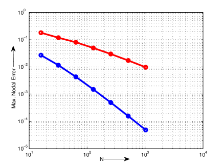
Figure 1: Loglog plot of the maximum nodal errors with $\varepsilon=10^{-9}$ correspond to finite difference scheme 3.1 (blue line) and the upwind scheme [20] (red line) for Example 1

Numerical results presented in Tables 1-4 show that the accuracy of the proposed finite difference scheme is in good agreement with the theoretical prediction. We apply both the forward midpoint upwind and backward midpoint upwind operator depending upon the sign $a(x)$ to tackle the stability of the proposed finite difference scheme. Table 1 and Table 3 display the maximum pointwise error and order of convergence for Example 1 and Example 2 respectively for different value of $\varepsilon$ and $N$. Table 1 and Table 3 indicate that the order of convergence of presented fitted mesh finite difference scheme (3.1) is one for $\varepsilon\geq 10^{-1}$ and almost of order two upto a logarithmic factor for $\varepsilon<10^{-1}$. It happens because for moderate value of $\varepsilon$, $i.e.,$ for $\varepsilon>N^{-1}$, midpoint upwind operator is first order convergent as given in Theorem 4.1 and in this case error correspond to the midpoint upwind operator dominates the error correspond to the central difference operator. Numerical results given in Tables 1-4 also show that the maximum nodal errors decreases and order of convergence increases as the number of mesh point increases. One can observe that as $\varepsilon$ is getting smaller for a particular value of mesh points $N$, both the maximum pointwise error and order of convergence are going to stabilized.

A comparison given in Table 1 for $\varepsilon=10^{-9}$, clearly indicate that the maximum pointwise errors are much smaller and order of convergence is much larger in this article than those obtained in [20] using upwind finite difference operator. It verify numerically the theoretical estimates that hybrid finite difference scheme (3.1) is second order $\varepsilon$-uniform convergent as opposed to the first order uniform convergence of upwind finite difference scheme [20] for turning point problems. We have not made comparison of numerical results for Example 2 with the finite difference scheme given in [20] because of authors used double mesh principle instead of analytical solution to get pointwise errors in [20]. Thus with almost same computational effort, proposed finite difference scheme gives more accuracy and rapid convergence then the finite difference scheme [20]. We also compare proposed finite difference scheme with the spline based numerical methods [11, 12, 13] numerically for both the Examples 1-2 and found that present scheme produce lesser pointwise errors and larger order of convergence than the spline based numerical methods [11, 12, 13]. Furthermore, one can see, Example 1 is analogous to the Testproblem 1 in [4] and our results are comparable to those extrapolation results in  [4] as both numerical schemes are of almost second order convergence $O(N^{-2}\ln(N)^{2})$ under the common assumption $\varepsilon\leq CN^{-1}$ for a given number of mesh points $N$.

In Figure 1, the Loglog graph of maximum pointwise errors is given correspond to the proposed scheme (blue line) and upwind finite difference scheme [20] (red line). This plot also indicate that the error of our scheme diminishing at the rate of $1/N^{2}$ while error correspond to scheme [20] approaches to zero almost as $1/N\rightarrow 0$. Thus all numerical evidences support our theoretical estimates.

References

• [1] L. Abrahamsson, “A priori estimates for solutions of singular perturbations with a turning point”, Stud. Appl. Math. 56 (1977) 51-69.
• [2] R.C. Ackerberg and R.E. O’Malley, “Boundary layer problems exhibiting resonance”, Stud. Appl. Math. 49 (1970) 277-295.
• [3] A. Berger, H. Han and R. Kellog,“ A priori estimates and analysis of a numerical method for a turning point problem”, Math. Comp. 42(1984) 465-492.
• [4] S. Becher and H.G. Roos, “Richardson extrapolation for a singularly perturbed turning point problem with exponential boundary layers”, J. Comput. Appl. Math. 290 (2015) 334-351.
• [5] F. Black and M. Scholes, “The price of options and corporate liabilites” J. Pol. Econ. 81(1973) 637-659.
• [6] P.A. Farrell,“Sufficient conditiond for the uniform convergence of a difference scheme for a singularly perturbed turning point problem”, SIAM J. Numer. Anal. 25(1988) 618-643.
• [7] D. Jingde, “Singularly perturbed boundary value problems for linear equations with turning points”, J. Math. Anal. Appl. 155(1991) 322-337.
• [8] S.Y. Hahn, J. Bigeon, and J.C. Sabonnadiere, “An ‘upwind’ finite element method for electromagnetic field problems in moving media”, Int. J. Numer. Methods Eng. 24(1987) 2071-2086.
• [9] C. Hirsch, “Numerical computation of internal and external flows”, Vol. 1. Wiley, Chichester 1988.
• [10] M. Jacob, “ Heat transfer.”, Wiley, New York, 1959.
• [11] M.K. Kadalbajoo and K.C. Patidar,“ Variable mesh spline approximation method for solving singularly perturbed turning point problems having boundary layer(s)”, Comp. Math. Appl. 42(2001) 1439-1453.
• [12] M.K. Kadalbajoo and V. Gupta, “A parameter uniform B-spline collocation method for solving singularly perturbed turning point problem having twin boundary layers”, Intern. J. Comput. Math. 87(2010) 3218-3235.
• [13] M.K. Kadalbajoo, P. Arora and V. Gupta, “Collocation method using artificial viscosity for solving stiff singularly perturbed turning point problem having twin boundary layers”, Comp. Math. Appl. 61(2011) 1595-1607.
• [14] R.B. Kellog and A. Tsan,“ Analysis of some difference approximations for a singular perturbation problem without turning points”, Math. Comp. 32(1978) 1025-1039.
• [15] B.E. Launder and B. Spalding, “Mathematical models of turbulence”, Academic press, New York 1972.
• [16] R.E. O’Malley,“ Introduction to Singular Perturbations”, Academic Press, New York, 1974.
• [17] R.E. O’Malley,“ Singular Perturbation for Ordinary Differential Equations”, Springer-Verlag, New York, 1991.
• [18] J.B. Munyakazi and K.C. Patidar, “Performance of Richardson extrapolation on some numerical methods for a singularly perturbed turning point problem whose solution has boundary layers”, J. Korean Math. Soc. 51 (4) (2014) 679-702.
• [19] J.B. Munyakazi, K.C. Patidar and M.T. Sayi, “A robust fitted operator finite difference method for singularlyperturbed problems whose solution has an interior layer”, Mathematics and Computers in Simulation, 160 (2019) 155-167.
• [20] S. Natesan, J. Jayakumar and J. Vigo Aguiar, “Parameter uniform numerical method for singularly perturbed turning point problems exhibiting boundary layers”, J. Comput. Appl. Math. 158 (2003) 121-134.
• [21] S. Polak, C. Den Heiger, W.H. Schilders and P. Markowich, “Semiconductor device modelling from the numerical point of view ”, Int. J. Numer. Methods Eng. 24(1987) 763-838.
• [22] K.K. Sharma, P. Rai and K.C. Patidar, “A review on singularly perturbed differential equations with turning points and interior layers”, Appl. Math. Comput. 219 (2013), 10575-10609.
• [23] M. Stynes and H.G. Roos, “The midpoint upwind scheme”, Appl. Numer. Math. 23 (1997), 361-374.
• [24] W. Wasow,“Linear turning point theory”, Springer, New York,1985.