A Chebyshev Spectral Method for Nonlinear Fourier Transform: Norming Constants

Abstract

In this paper, we present a Chebyshev based spectral method for the computation of the Jost solutions corresponding to complex values of the spectral parameter in the Zakharov–Shabat scattering problem. The discrete framework is then used to devise a new algorithm based on a minimum total variation (MTV) principle for the computation of the norming constants which comprise the discrete part of the nonlinear Fourier spectrum. The method relies on the MTV principle to find the points where the expressions for norming constants are numerically well-conditioned.

I Introduction

This paper considers the Zakharov and Shabat (ZS) [1] scattering problem which forms the basis for defining a nonlinear generalization of the conventional Fourier transform dubbed as the nonlinear Fourier transform (NFT). In an optical fiber communication system the nonlinear Fourier (NF) spectrum offers a novel way of encoding information in optical pulses where the nonlinear effects are adequately taken into account as opposed to being treated as a source of signal distortion [2, 3]. One of the challenges that has emerged in realizing these ideas is the development of a fast and well-conditioned NFT algorithm that can offer spectral accuracy at low complexity. Such an algorithm would prove extremely useful for system design and benchmarking. Currently, there are primarily two successful approaches proposed in the literature for computing the continuous NF spectrum which are capable of achieving algebraic orders convergence at quasilinear complexity: (a) the integrating factor (IF) based exponential integrators [4, 5, 6, 7, 8] (b) exponential time differencing (ETD) method based exponential integrators [9]. Note that while the IF schemes uses fast polynomial arithmetic in the monomial basis, the ETD schemes use fast polynomial arithmetic in the Chebyshev basis. For the inverse transform, a sampling series based approach for computing the “radiative” part has been proposed in [10] which achieves spectral accuracy at quasilinear complexity per sample of the signal. In this paper, we extend the recently proposed spectral method [11] for the computation continuous spectrum to compute the norming constants. It is well-known that the determination of the point where the expression which defines the norming constant is numerically well-conditioned is non-trivial problem. In the previous works [5, 6, 7] this point was taken to be origin, however, this choice can be shown to fail for carefully constructed examples. In order to remedy this problem, we propose a minimum total variation (MTV) principle to determine a set of points where the expression for the norming constants are well-conditioned. Note that total variation of the quantities in question are identically zero at the continuous level; therefore, it makes sense to seek the minima of TV for a sliding window of fixed size which traverses the sampling grid. The size of the sliding window can be adaptively reduced which adds to the effectiveness of the algorithm.

We begin our discussion with a brief review of the scattering theory closely following the formalism presented in [12]. The nonlinear Fourier transform of any signal is defined via the Zakharov-Shabat (ZS) [1] scattering problem which can be stated as follows: For $\zeta\in\mathbb{R}$ and $\bm{v}=(v_{1},v_{2})^{\intercal}$,

$$\bm{v}_{t}=-i\zeta\sigma_{3}\bm{v}+U(t)\bm{v},$$ (1)

where $\sigma_{3}$ is one of the Pauli matrices defined in the beginning of this article. The potential $U(t)$ is defined by $U_{11}=U_{22}=0,\,U_{12}=q(t)$ and $U_{21}=-q^{*}(t)$. Here, $\zeta\in\mathbb{R}$ is known as the spectral parameter and $q(t)$ is the complex-valued signal. The solution of the scattering problem (1), henceforth referred to as the ZS problem, consists in finding the so called scattering coefficients which are defined through special solutions of (1) known as the Jost solutions which are linearly independent solutions of (1) with a prescribed behavior at $+\infty$ or $-\infty$. The Jost solutions of the first kind, denoted by $\bm{\psi}(t;\zeta)$ and $\overline{\bm{\psi}}(t;\zeta)$, are the linearly independent solutions of (1) which have the following asymptotic behavior as $t\rightarrow\infty$: $\bm{\psi}(t;\zeta)e^{-i\zeta t}\rightarrow(0,1)^{\intercal}$ and $\overline{\bm{\psi}}(t;\zeta)e^{i\zeta t}\rightarrow(1,0)^{\intercal}$. The Jost solutions of the second kind, denoted by $\bm{\phi}(t;\zeta)$ and $\overline{\bm{\phi}}(t;\zeta)$, are the linearly independent solutions of (1) which have the following asymptotic behavior as $t\rightarrow-\infty$: $\bm{\phi}(t;\zeta)e^{i\zeta t}\rightarrow(1,0)^{\intercal}$ and $\overline{\bm{\phi}}(t;\zeta)e^{-i\zeta t}\rightarrow(0,-1)^{\intercal}$. The scattering coefficients are defined by

$$\begin{split}&\mathfrak{a}(\zeta)=\operatorname{\mathscr{W}}\left(\bm{\phi},{\bm{\psi}}\right),\quad\mathfrak{b}(\zeta)=\operatorname{\mathscr{W}}\left(\overline{\bm{\psi}},\bm{\phi}\right),\\ &\overline{\mathfrak{a}}(\zeta)=\operatorname{\mathscr{W}}\left(\overline{\bm{\phi}},\overline{\bm{\psi}}\right),\quad\overline{\mathfrak{b}}(\zeta)=\operatorname{\mathscr{W}}\left(\overline{\bm{\phi}},{\bm{\psi}}\right),\end{split}$$ (2)

for $\zeta\in\mathbb{R}$. The analytic continuation of the Jost solution with respect to $\zeta$ is possible provided the potential is decays sufficiently fast or has a compact support. If the potential has a compact support, the Jost solutions have analytic continuation in the entire complex plane. Consequently, the scattering coefficients $\mathfrak{a}(\zeta)$, $\mathfrak{b}(\zeta)$, $\overline{\mathfrak{a}}(\zeta)$, $\overline{\mathfrak{b}}(\zeta)$ are analytic functions of $\zeta\in\mathbb{C}$ [12].

In general, the nonlinear Fourier spectrum for the signal $q(t)$ comprises a discrete and a continuous spectrum. The discrete spectrum consists of the so called eigenvalues $\zeta_{k}\in\mathbb{C}_{+}$, such that $\mathfrak{a}(\zeta_{k})=0$, and, the norming constants $b_{k}$ such that $\bm{\phi}(t;\zeta_{k})=b_{k}\bm{\psi}(t;\zeta_{k})$. For compactly supported potentials, $b_{k}=b(\zeta_{k})$. The continuous spectrum, also referred to as the reflection coefficient, is defined by $\rho(\xi)={\mathfrak{b}(\xi)}/{\mathfrak{a}(\xi)}$ for $\xi\in\mathbb{R}$.

II The numerical scheme

Introducing the “local” scattering coefficients $a(t;\zeta)$ and $\breve{b}(t;\zeta)$ such that $\bm{\phi}(t;\zeta)e^{i\zeta t}=(a(t;\zeta),\breve{b}(t;\zeta))^{\intercal}$, the ZS scattering problem can be written as $\partial_{t}a(t;\zeta)=q(t)\breve{b}(t;\zeta)$ and $\partial_{t}\breve{b}(t;\zeta)-2i\zeta\breve{b}(t;\zeta)=r(t)a(t;\zeta)$. Let the scattering potential $q(t)$ be supported in $\mathbb{I}=[-1,1]$. Such signals have been studied in more detail in [5, 13, 14, 15] also in order to understand the consequence of domain truncation for general signals. For $\zeta\in\mathbb{C}_{+}$, the ‘initial’ conditions for the Jost solution $\bm{\phi}$ are: $a(-1;\zeta)=1$ and $\breve{b}(-1;\zeta)=0$. The scattering coefficients $\mathfrak{a}$ and $\mathfrak{b}$ are given by $\mathfrak{a}(\zeta)=a(+1;\zeta)$ and $\mathfrak{b}(\zeta)=\breve{b}(+1;\zeta)e^{-2i\zeta}$. In the following, we describe a numerical scheme based on the Chebyshev polynomials to solve the coupled Volterra integral equations

$$\begin{split}&a(t;\zeta)=1+\int_{-1}^{t}q(s)\breve{b}(s;\zeta)ds,\\ &\breve{b}(t;\zeta)=2i\zeta\int^{t}_{-1}\breve{b}(s;\zeta)ds+\int_{-1}^{t}r(s)a(s;\zeta)ds,\end{split}$$ (3)

which are equivalent to the ZS problem with the aforementioned initial conditions. The numerical scheme computes the approximations to the Jost solutions in terms of the Chebyshev polynomials which can then used to compute the scattering coefficients. In the following, for the sake of brevity of presentation, we assume that the eigenvalues are known. The method of computing the eigenvalues using a Chebyshev based spectral would be presented in a future publication. Here we focus entirely on the computation of the norming constants. In principle, the norming constants can be computed simply by evaluating the numerical approximation to $\mathfrak{b}(\zeta)$ at the eigenvalue $\zeta_{k}$ to obtain $b_{k}$, however, $\breve{b}(+1;\zeta_{k})$ becomes negligibly small which must now be multiplied with $\exp(-2i\zeta_{k})$ which grows exponentially. These intermediate quantities can easily suffer from lack of precision leading to inaccurate determination of $b_{k}$.

Let $c(t)=\sum_{n=0}^{\infty}C_{n}T_{n}(t)$. Following [11], the integral operator $\mathscr{K}$ defined by $\mathscr{K}[c](t)=\int_{-1}^{t}c(s)ds=d(t)$ in the Chebyshev basis is given by

$$d(t)=\left[C_{0}-\frac{1}{4}C_{1}-\sum_{n=2}^{\infty}\frac{(-1)^{n}C_{n}}{n^{2}-1}\right]T_{0}(t)\\ +\left[C_{0}-\frac{1}{2}C_{2}\right]T_{1}(t)+\sum_{n=2}^{\infty}\frac{1}{2n}\left[C_{n-1}-C_{n+1}\right]T_{n}(t).$$ (4)

In the matrix form, $\mathscr{K}$ has the representation

$$\mathcal{K}=\begin{pmatrix}1&-\frac{1}{4}&-\frac{1}{3}&+\frac{1}{8}&-\frac{1}{15}&\ldots\\ 1&0&-\frac{1}{2}&&&\\ &\frac{1}{4}&0&-\frac{1}{4}&&\\ &&\frac{1}{6}&0&-\frac{1}{6}&\\ &&&\ddots&\ddots&\ddots\end{pmatrix}.$$ (5)

The next step in the discretization of (3) involves expanding the signal in the Chebyshev basis. Let $q(t)=\sum_{n=0}^{\infty}Q_{n}T_{n}(t)$ and $r(t)=\sum_{n=0}^{\infty}R_{n}T_{n}(t)$ where $R_{n}=-Q^{*}_{n}$. A truncated expansion upto $N$ terms can be accomplished by sampling the potentials at the Chebyshev–Gauss–Lobatto (CGL) nodes given by $t_{n}=-\cos[n\pi/(N-1)],\,n=0,1,\ldots N-1$ and carrying out discrete Chebyshev transform which can be implemented using an FFT of size $2(N-1)$ [16].

Figure 1: The sparsity pattern of a truncated version of the matrix $\mathcal{S}$ where $M^{\prime}=M+1$ with $M$ being the number of Chebyshev polynomials used for approximating $q(t)$.

Now, our final goal is to obtain an expansion of the local scattering coefficients in the Chebyshev basis: To this end, let $a(t;\zeta)=\sum_{n=0}^{\infty}A_{n}T_{n}(t)$ and $\breve{b}(t;\zeta)=\sum_{n=0}^{\infty}B_{n}T_{n}(t)$ where $A_{n}$ and $B_{n}$ are to be determined (for fixed value of $\zeta$). The last ingredient needed in the discretization of (3) are the products $r(t)a(t;\zeta)$ and $q(t)\breve{b}(t;\zeta)$ which must be represented as linear operations on the unknown coefficient vectors $\bm{A}=(A_{0},A_{1},\ldots)^{\intercal}$ and $\bm{B}=(B_{0},B_{1},\ldots)^{\intercal}$. Again following [11], let $r(t)a(t;\zeta)=\sum_{l=0}^{\infty}G_{l}T_{l}(t)$ and $q(t)\breve{b}(t;\zeta)=\sum_{l=0}^{\infty}H_{l}T_{l}(t)$; then, $2G_{0}=2R_{0}A_{0}+\sum_{k=1}^{\infty}R_{k}A_{k}$, $2H_{0}=2Q_{0}B_{0}+\sum_{k=1}^{\infty}Q_{k}B_{k}$ and

$$\begin{split}2G_{l}&=\sum_{k=0}^{l-1}R_{l-k}A_{k}+2R_{0}A_{l}+\sum_{k=1}^{\infty}R_{k}A_{k+l}+\sum_{k=0}^{\infty}R_{k+l}A_{k},\\ 2H_{l}&=\sum_{k=0}^{l-1}Q_{l-k}B_{k}+2Q_{0}B_{l}+\sum_{k=1}^{\infty}Q_{k}B_{l+k}+\sum_{k=0}^{\infty}Q_{k+l}B_{k}.\end{split}$$ (6)

for $l\in\mathbb{N}$. These relations define the operator $\mathcal{M}[\bm{Q}]$, which comprises a Töplitz and an almost Hankel matrix given by

$$2\mathcal{M}[\bm{Q}]=\begin{pmatrix}2Q_{0}&Q_{1}&Q_{2}&\cdots\\ Q_{1}&2Q_{0}&Q_{1}&\ddots\\ Q_{2}&Q_{1}&2Q_{0}&\ddots\\ \vdots&\ddots&\ddots&\ddots\end{pmatrix}\\ +\begin{pmatrix}0&0&0&\cdots\\ Q_{1}&Q_{2}&Q_{3}&\reflectbox{$\ddots$}\\ Q_{2}&Q_{3}&Q_{4}&\reflectbox{$\ddots$}\\ \vdots&\reflectbox{$\ddots$}&\reflectbox{$\ddots$}&\reflectbox{$\ddots$}\end{pmatrix},$$ (7)

Similarly, the representation of the operator $\mathcal{M}[\bm{R}]$ can be defined. Setting $\Lambda=\mathcal{K}\mathcal{M}[\bm{Q}]$, the discrete version of (3) can be stated as

$$\begin{pmatrix}I&-\Lambda\\ \Lambda^{*}&I-2i\zeta\mathcal{K}\end{pmatrix}\begin{pmatrix}\bm{A}\\ \bm{B}\end{pmatrix}=\mathcal{S}\begin{pmatrix}\bm{A}\\ \bm{B}\end{pmatrix}=\begin{pmatrix}\bm{E}_{0}\\ \bm{0}\end{pmatrix},$$ (8)

where $I$ is the identity matrix, $\bm{E}_{0}=(1,0,\ldots)^{\intercal}$ and $\bm{0}=(0,0,\ldots)^{\intercal}$. Noting that $\bm{A}=\bm{E}_{0}+\Lambda\bm{B}$ and setting $\Gamma=\Lambda^{*}\Lambda$, we have $\left(I-2i\zeta\mathcal{K}+\Gamma\right)\bm{B}=\mathcal{K}\bm{R}$ where we have used the fact that $\mathcal{M}[\bm{R}]\bm{E}_{0}=\bm{R}$. The numerical scheme can be obtained as follows: truncation of the Chebyshev expansion of $q(t)$ to $M$ terms, truncation of $\bm{E}_{0}$, $\bm{A}$ and $\bm{B}$ to $N$-dimensional vectors, and, truncation of $\Lambda$ and $\mathcal{K}$ to $N\times N$ matrix where $N\geq 2M$. If a direct sparse solver is used, the complexity of the numerical scheme would be lower than $\mathop{\mathscr{O}}\left(N^{3}\right)$.

Remark II.1.

Let us remark that within the iterative approach and using the structured nature of the matrices involved it is possible to lower the complexity of the linear solver as in [11]. Our preliminary investigation indicate that the formulation

$$\left[I+\left(I-2i\zeta\mathcal{K}\right)^{-1}\Gamma\right]\bm{B}=\left(I-2i\zeta\mathcal{K}\right)^{-1}\mathcal{K}\bm{R},$$ (9)

works better for iterative solvers. However, the number of iterations needed for the stabilized biconjugate gradient method [17] can be as large as $50$. Let us also mention that fast versions of the direct solvers for banded systems with certain number of filled first rows have been proposed [18]. We defer these aspects to a future publication.

The recipe discussed above accomplishes the computation of the Jost function of second kind $\bm{\phi}$, let us now show that by solving the scattering problem in the setting described above for $q^{*}(-t)$ it is possible to compute the Jost solution of the first kind $\bm{\psi}$. If $\bm{\Phi}(t;\zeta)$ denotes the Jost solution of the second kind for $q^{*}(-t)$, we have $\bm{\psi}(t;\zeta)=(\Phi_{2}(-t;\zeta),\Phi_{1}(-t;\zeta))^{\intercal}$ [5]. For convenience, let $\bm{\psi}(t;\zeta)e^{-i\zeta t}=(\breve{c}(t;\zeta),d(t;\zeta))^{\intercal}$ so that, for $\zeta\in\mathbb{C}_{+}$, the ‘initial’ conditions are: $d(1;\zeta)=1$ and $\breve{c}(1;\zeta)=0$. The scattering coefficients $\mathfrak{a}$ and $\overline{\mathfrak{b}}$ are given by $\mathfrak{a}(\zeta)=d(-1;\zeta)$ and $\overline{\mathfrak{b}}(\zeta)=\breve{c}(-1;\zeta)e^{-2i\zeta}$. Again, we do not attempt to evaluate $\overline{\mathfrak{b}}$ at the eigenvalues $\zeta_{k}$. Finally, let us note that the Chebyshev coefficients of $q^{*}(-t)$ are given by $(-1)^{n}Q_{n},\,n\in\mathbb{N}_{0},$ which follows from the symmetry property of the Chebyshev polynomials: $T_{n}(-t)=(-1)^{n}T_{n}(t)$.

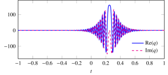
Figure 2: The figure shows a chirped hyperbolic signal for which the parameters are $\mu=0.8$, $K=8$, $A_{0}=K/\lambda\approx 16.66$ and $t_{0}=0.25$. The scaling parameter is $W=12$.

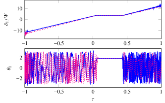
Figure 3: The figure shows $\delta_{1}$ (top) and $\theta_{1}$ (bottom) computed for the signal in Fig. 2 from the expressions defined in (11), namely, $f_{\delta}$ (solid line) and $g_{\delta}$ (dotted line) for $\delta_{1}$, and, $f_{\theta}$ (solid line), $g_{\theta}$ (dotted line) for $\theta_{1}$ where the corresponding eigenvalue is $\zeta_{1}=i9.5W$. The MTV algorithm (applied to $f_{\delta}$ and $g_{\delta}$) with sliding-window size $m=20$ yields $\tau=0.24,0.26$ for which the errors are as follows: $|\delta_{1}-\delta^{(\text{num.})}_{1}|=1.16\times 10^{-7},1.16\times 10^{-7}$, $|\theta_{1}-\theta_{1}^{(\text{num.})}|=1.77\times 10^{-7},1.77\times 10^{-7}$, respectively.

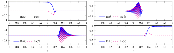
Figure 4: The figure shows the numerically computed (modified) Jost solutions for the signal shown in Fig. 2 corresponding to the eigenvalue $\zeta_{1}=i9.5W$ with numerical parameters given by $M=2^{9}$ and $N=2^{11}$. The quality of the approximation can be assessed from $|\mathfrak{a}^{(\text{num.})}(\zeta_{1})|\approx 3.36\times 10^{-16}$.

Having discussed the computation of the Jost solutions, we turn to the computation of the norming. To this end, let $\zeta_{k}=i\xi_{k}+\eta_{k}$. For convenience, we set $b_{k}=\exp(i\theta_{k}+\delta_{k})$ and introduce the functions

$$\begin{split}&f_{\delta}(\tau;\zeta_{k})=\ln\left|\frac{a(\tau;\zeta_{k})}{\breve{c}(\tau;\zeta_{k})}\right|+2\operatorname{Im}{\zeta_{k}}\tau,\\ &g_{\delta}(\tau;\zeta_{k})=\ln\left|\frac{\breve{b}(\tau;\zeta_{k})}{d(\tau;\zeta_{k})}\right|+2\operatorname{Im}{\zeta_{k}}\tau,\\ &f_{\theta}(\tau;\zeta_{k})=\arg\left[\frac{a(\tau;\zeta_{k})}{\breve{c}(\tau;\zeta_{k})}e^{-2i\operatorname{Re}{\zeta_{k}}\tau}\right]\\ &g_{\theta}(\tau;\zeta_{k})=\arg\left[\frac{\breve{b}(\tau;\zeta_{k})}{d(\tau;\zeta_{k})}e^{-2i\operatorname{Re}{\zeta_{k}}\tau}\right],\end{split}$$ (10)

so that

$$\delta_{k}=f_{\delta}(\tau;\zeta_{k})=g_{\delta}(\tau;\zeta_{k}),\quad\theta_{k}=f_{\theta}(\tau;\zeta_{k})=g_{\theta}(\tau;\zeta_{k}),$$ (11)

for $\tau\in\mathbb{I}$. The functions defined above are constant with respect to $\tau$ for any given eigenvalue $\zeta_{k}$, however, at the discrete level they may vary. The choice of $\tau$ where the expressions above must be evaluated depends on the numerical conditioning of the quantities involved. Let a sub-grid $J$ be said to be admissible with respect to $f_{\delta}$ if its total variation over $J$, given by

$$\begin{split}\mathscr{V}[f_{\delta};J]=\sum_{n}|f_{\delta}(\tau_{n+1};\zeta_{k})-f_{\delta}(\tau_{n};\zeta_{k})|,\end{split}$$ (12)

satisfies the condition $\mathscr{V}[f_{\delta};J]\leq\epsilon,(\epsilon>0)$. In the numerical implementation, we introduce a sliding window given by $J_{n}(m)=\{\tau_{n},\tau_{n+1},\ldots,\tau_{n+m-1}\}$ where $m<N$ is fixed. If an appropriate tolerance $\epsilon$ cannot be guessed a priori, we simply choose $J_{m}(n)$ that corresponds to $\min_{n}\mathscr{V}[f_{\delta};J_{m}(n)]$. The point $\tau_{n+m/2}$ can then be reported as the optimal point for the computation of $\delta$ and $\theta$. We label this algorithm as the minimum total variation (MTV) algorithm.

III Numerical Tests

For numerical tests, we consider the chirped secant-hyperbolic potential [19] given by $q(t)=Wf((t-t_{0})/W)$ for $t\in\mathbb{I}$ where

$$f(s)=A_{0}{\exp[-2i\mu A_{0}\log(\cosh s)]}/{\cosh(s)},\quad s\in\mathbb{R}.$$ (13)

Here, $W>0$ controls how well the signal $q(t)$ is supported in $\mathbb{I}$. Let $\mu\in[0,1)$ and $\lambda=\sqrt{1-\mu^{2}}\in(0,1]$ and set $\omega=\lambda+i\mu\in\mathbb{T}$. Further, set $\tilde{A}_{0}=\lambda A_{0}+{1}/{2}$ and let $K=\left\lfloor\tilde{A}_{0}\right\rfloor$; then, the eigenvalues are given by $\zeta_{k}=i\left(\tilde{A}_{0}-k\right)W$ and the corresponding norming constants are given by

$$b_{k}=\omega e^{-2i\mu A_{0}(\log 2)+i\pi k}\prod_{j=1}^{k-1}\left(\frac{\omega A_{0}-j}{\omega^{*}A_{0}-j}\right)e^{2i\zeta_{k}t_{0}},$$ (14)

for $k=1,2,\ldots,K$. We set $\tilde{A}_{0}=K+1/2$ so that $A_{0}=K/\lambda$ and

$$\zeta_{k}=i\left(K+1/2-k\right)W,\quad k=1,2,\ldots,K.$$ (15)

The signal for the choice of parameters $W=12$, $\mu=0.8$, $t_{0}=0.25$ and $K=8$ is shown in Fig. 2. The two expression for $\delta_{1}$ and $\theta_{1}$ provided in (11) are plotted in Fig. 3 which correspond to the numerically computed Jost solution for $\zeta_{1}$ shown in Fig. 4 with $M=2^{9}$ and $N=4M$. It is evident from Fig. 3 that the choice of $\tau$ is non-trivial and the choice of $\tau=0$ is certainly not admissible. The MTV algorithm applied to the functions $f_{\delta}$ and $g_{\delta}$ with sliding-window size $m=20$ finds the optimal points to be $\tau=0.24,0.26$, respectively. The errors $|\delta_{1}-\delta^{(\text{num.})}_{1}|$ and $|\theta_{1}-\theta_{1}^{(\text{num.})}|$ for each of the choices of $\tau$ are of the order $10^{-7}$.

A second example to demonstrate the effectiveness of the MTV algorithm is that of an $8$-soliton solution whose discrete spectrum in terms of the triplets $(\zeta_{k},\delta_{k},\theta_{k})$ is listed in Table I. The signal computed using the classical Darboux transformation [20, 5, 14, 15] for the choice $W=10$ is shown in Fig. 5 and numerically computed Jost solutions in Fig. 6. The two expression for $\delta_{1}$ and $\theta_{1}$ provided in (11) are plotted in Fig. 7 which correspond to the numerically computed Jost solution for $\zeta_{1}$ with $M=2^{9}$ and $N=4M$. It is evident from Fig. 7 that the choice of $\tau$ is again non-trivial and the choice of $\tau=0$ is once again not admissible. The MTV algorithm applied to the functions $f_{\delta}$ and $g_{\delta}$ with sliding-window size $m=20$ finds the optimal points to be $\tau\approx 0.29,0.34$, respectively. The errors $|\delta_{1}-\delta^{(\text{num.})}_{1}|$ and $|\theta_{1}-\theta_{1}^{(\text{num.})}|$ for each of the choices of $\tau$ are of the order $10^{-7}$.

The third example to demonstrate the effectiveness of the MTV algorithm is derived from the last example by multiplying a linear phase factor $\exp(i2\xi_{\text{shift}}t)$ to the signal so that the eigenvalues acquire a shift of $\xi_{\text{shift}}$ which we choose to set $4\operatorname{Re}{\zeta_{1}}$ (see Table I). We let the numerical parameters to be the same as in the last example. The signal shown in Fig. 8, the variation of $\delta_{1},\theta_{1}$ are shown in Fig. 9 which correspond to the numerically computed Jost solution (see Fig. 10) for $\zeta_{1}+4\operatorname{Re}{\zeta_{1}}$. The MTV algorithm applied to the functions $f_{\delta}$ and $g_{\delta}$ finds the optimal points to be $\tau\approx 0.25,0.36$, respectively. The errors $|\delta_{1}-\delta^{(\text{num.})}_{1}|$ and $|\theta_{1}-\theta_{1}^{(\text{num.})}|$ for each of the choices of $\tau$ are of the order $10^{-4}$ and $10^{-5}$, respectively.

TABLE I: Discrete spectrum

$k$	$\zeta_{k}/W$	$\theta_{k}$	$\delta_{k}$
$1$	$-2.5+4.33013i$	$2.74889$	$+16$
$2$	$+2.5+4.33013i$	$2.35619$	$-16$
$3$	$-2+3.4641i$	$1.9635$	$+16$
$4$	$+2+3.4641i$	$1.5708$	$-16$
$5$	$-1.5+2.59808i$	$1.1781$	$+16$
$6$	$+1.5+2.59808i$	$0.785398$	$-16$
$7$	$-1+1.73205i$	$0.392699$	$+16$
$8$	$+1+1.73205i$	$0$	$-16$

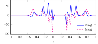
Figure 5: The figure shows the $8$-soliton solution corresponding to the discrete spectrum listed in Table I. The scaling parameter is $W=10$.

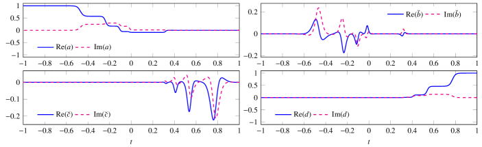
Figure 6: The figure shows the numerically computed (modified) Jost solutions for the signal shown in Fig. 5 corresponding to the eigenvalue $\zeta_{1}/W=-2.5+4.33013i$ with numerical parameters given by $M=2^{9}$ and $N=2^{11}$. The quality of the approximation can be assessed from $|\mathfrak{a}^{(\text{num.})}(\zeta_{1})|\approx 2.99\times 10^{-10}$.

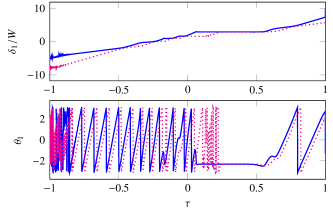
Figure 7: The figure shows $\delta_{1}$ (top) and $\theta_{1}$ (bottom) computed for the signal in Fig. 5 from the expressions defined in (11), namely, $f_{\delta}$ (solid line) and $g_{\delta}$ (dotted line) for $\delta_{1}$, and, $f_{\theta}$ (solid line), $g_{\theta}$ (dotted line) for $\theta_{1}$ where the corresponding eigenvalue is $\zeta_{1}/W=-2.5+4.33013i$. The MTV algorithm (applied to $f_{\delta}$ and $g_{\delta}$) with sliding-window size $m=20$ yields $\tau\approx 0.29,0.34$ for which the errors are as follows: $|\delta_{1}-\delta^{(\text{num.})}_{1}|=7.74\times 10^{-7},5.29\times 10^{-7}$, $|\theta_{1}-\theta_{1}^{(\text{num.})}|=4.74\times 10^{-7},8.51\times 10^{-7}$, respectively.

The final numerical tests are meant to verify the spectral convergence of the numerical scheme. To this end, we quantify the error by

$$e_{\theta}=\frac{1}{K}\sum_{k=1}^{K}|\theta_{k}-\theta^{\text{num.}}_{k}|,\quad e_{\delta}=\frac{1}{K}\sum_{k=1}^{K}|\delta_{k}-\delta^{\text{num.}}_{k}|.$$ (16)

We set $N=4M$ and consider the set of values $K\in\{4,8,12,16\}$.

The first profile we would like to use for the convergence analysis is chirped hyperbolic profile. Let us set the parameters as $\mu=0.8$, $t_{0}=0$ and $W=20$. The choice of these parameters makes $\tau=0$ optimal for the computation of the norming constants. The results of the convergence analysis is shown in Fig. 11 which confirms the spectral convergence of the numerical scheme. The plateauing of the error seen in these plots are on account of the lack of compact support of $q(t)$.

The second profile we would like to use for the convergence analysis are multisoliton solutions. Let $\theta_{j}=\pi(j+2)/9\in[\pi/3,2\pi/3]$ for $j=1,\ldots,4$. Then the eigenvalues are defined as $\zeta_{j+4(l-1)}=l\exp(i\theta_{j}),\,l=1,\ldots,4,\,j=1,\ldots,4$. The norming constants are chosen as $b_{j}=\exp[i\pi(j-1)/16],\,j=1,2,\ldots,16$. The discrete spectrum corresponding to $K=16$ is depicted in Fig. 12. The potential can be computed with machine precision using the classical Darboux transformation algorithm [5]. The scaling parameter is set to be $W=22$. Here, $\tau=0$ is known to be optimal for the computation of the norming constants. The results of the convergence analysis is shown in Fig. 13 which confirms the spectral convergence of the numerical scheme. The plateauing of the error seen in these plots are again on account of the lack of compact support of $q(t)$.

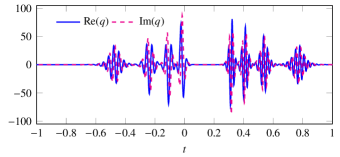
Figure 8: The figure shows a signal derived from the $8$-soliton solution corresponding to the discrete spectrum listed in Table I by multiplying a linear phase factor given by $\exp(i8\operatorname{Re}(\zeta_{1})t)$. The scaling parameter is $W=10$.

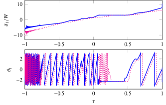
Figure 9: The figure shows $\delta_{1}$ (top) and $\theta_{1}$ (bottom) computed for the signal in Fig. 8 from the expressions defined in (11), namely, $f_{\delta}$ (solid line) and $g_{\delta}$ (dotted line) for $\delta_{1}$, and, $f_{\theta}$ (solid line), $g_{\theta}$ (dotted line) for $\theta_{1}$ where the corresponding eigenvalue is $\zeta_{1}/W=8.5+4.33013i$. The MTV algorithm (applied to $f_{\delta}$ and $g_{\delta}$) with sliding-window size $m=20$ yields $\tau\approx 0.25,0.36$ for which the errors are as follows: $|\delta_{1}-\delta^{(\text{num.})}_{1}|=3.11\times 10^{-4},2.96\times 10^{-4}$, $|\theta_{1}-\theta_{1}^{(\text{num.})}|=9.64\times 10^{-7},2.44\times 10^{-5}$, respectively.

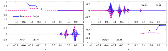
Figure 10: The figure shows the numerically computed (modified) Jost solutions for the signal shown in Fig. 8 corresponding to the eigenvalue $\zeta_{1}/W=8.5+4.33013i$. The quality of the approximation can be assessed from $|\mathfrak{a}^{(\text{num.})}(\zeta_{1})|\approx 8.20\times 10^{-9}$.

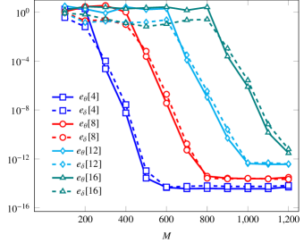
Figure 11: The figure shows the convergence analysis for the chirped secant hyperbolic profile with $\mu=0.8$, $t_{0}=0$ and the scaling parameter $W=20$. The legends depict the quantities $e_{\delta}[K]$ and $e_{\theta}[K]$ defined by (16) and parametrized by $K$, the number of eigenvalues.

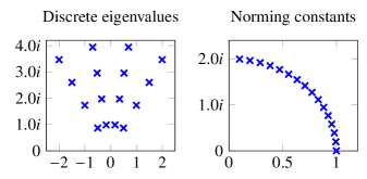
Figure 12: The figure shows the discrete spectrum of a multisoliton solution.

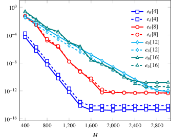
Figure 13: The figure shows the convergence analysis for multisoliton solutions with number of eigenvalues $K=4,8,12,16$ where the discrete spectrum in each of the cases is a subset of that shown in Fig. 12. The legends depict the quantities $e_{\delta}[K]$ and $e_{\theta}[K]$ defined by (16) and parametrized by $K$.

IV Conclusion

In this paper, we presented a Chebyshev spectral method for the solution of the Zakharov–Shabat scattering problem for complex values of the spectral parameter. Within this discrete framework, we also proposed a robust algorithm for computing the norming constants. This algorithm is based on a minimum total variation principle and therefore the algorithm is abbreviated as the MTV algorithm for norming constants. Future work in this direction will focus on developing fast solvers for the linear system within the direct (relying on the structured nature of the system matrix) as well as iterative (relying on the fast matrix–vector multiplication for structured matrices) methods with and without preconditioning.

References

• [1] V. E. Zakharov and A. B. Shabat, “Exact theory of two-dimensional self-focusing and one-dimensional self-modulation of waves in nonlinear media,” Sov. Phys. JETP, vol. 34, pp. 62–69, 1972.
• [2] M. I. Yousefi and F. R. Kschischang, “Information transmission using the nonlinear Fourier transform, Part I,” IEEE Trans. Inf. Theory, vol. 60, no. 7, pp. 4312–4369, 2014.
• [3] S. K. Turitsyn, J. E. Prilepsky, S. T. Le, S. Wahls, L. L. Frumin, M. Kamalian, and S. A. Derevyanko, “Nonlinear Fourier transform for optical data processing and transmission: advances and perspectives,” Optica, vol. 4, no. 3, pp. 307–322, 2017.
• [4] V. Vaibhav and S. Wahls, “Introducing the fast inverse NFT,” in Optical Fiber Communication Conference.   Los Angeles, CA, USA: Optical Society of America, 2017, p. Tu3D.2.
• [5] V. Vaibhav, “Fast inverse nonlinear Fourier transformation using exponential one-step methods: Darboux transformation,” Phys. Rev. E, vol. 96, p. 063302, 2017.
• [6] V. Vaibhav, “Fast inverse nonlinear Fourier transform,” Phys. Rev. E, vol. 98, p. 013304, 2018.
• [7] V. Vaibhav, “Higher order convergent fast nonlinear Fourier transform,” IEEE Photonics Technol. Lett., vol. 30, no. 8, pp. 700–703, 2018.
• [8] V.Vaibhav, “Efficient nonlinear Fourier transform algorithms of order four on equispaced grid,” IEEE Photonics Technol. Lett., vol. 31, no. 15, pp. 1269–1272, 2019.
• [9] V. Vaibhav, “Fast nonlinear Fourier transform using Chebyshev polynomials,” arXiv, 2019, arXiv:1908.09811[physics.comp-ph]. [Online]. Available: https://arxiv.org/abs/1908.09811
• [10] V. Vaibhav, “Nonlinearly bandlimited signals,” J. Phys. A: Math. Theor., vol. 52, no. 10, p. 105202, 2019.
• [11] V. Vaibhav, “A fast Chebyshev spectral method for nonlinear Fourier transform,” arXiv, 2019, arXiv:1909.03710[physics.comp-ph]. [Online]. Available: https://arxiv.org/abs/1909.03710
• [12] M. J. Ablowitz, D. J. Kaup, A. C. Newell, and H. Segur, “The inverse scattering transform - Fourier analysis for nonlinear problems,” Stud. Appl. Math., vol. 53, no. 4, pp. 249–315, 1974.
• [13] V. Vaibhav, “Nonlinear Fourier transform of time-limited and one-sided signals,” J. Phys. A: Math. Theor., vol. 51, no. 42, p. 425201, 2018.
• [14] V. Vaibhav, “Exact solution of the Zakharov–Shabat scattering problem for doubly-truncated multisoliton potentials,” Commun. Nonlinear Sci. Numer. Simul., vol. 61, pp. 22–36, 2018.
• [15] V. Vaibhav, “Darboux transformation: new identities,” Physica Scripta, vol. 94, no. 11, p. 115504, 2019.
• [16] P. Giorgi, “On polynomial multiplication in Chebyshev basis,” IEEE Trans. Comput., vol. 61, no. 6, pp. 780–789, 2011.
• [17] H. A. Van der Vorst, “Bi-CGSTAB: A fast and smoothly converging variant of Bi-CG for the solution of nonsymmetric linear systems,” SIAM J. Sci. Stat. Comput., vol. 13, no. 2, pp. 631–644, 1992.
• [18] S. Olver and A. Townsend, “A fast and well-conditioned spectral method,” SIAM Review, vol. 55, no. 3, pp. 462–489, 2013.
• [19] A. Tovbis et al., “On semiclassical (zero dispersion limit) solutions of the focusing nonlinear Schrödinger equation,” Commun. Pure Appl. Math., vol. 57, no. 7, pp. 877–985, 2004.
• [20] V. Vaibhav and W. Wahls, “Multipoint newton-type nonlinear Fourier transform for detecting multi-solitons,” in Optical Fiber Communication Conference.   Anaheim, CA, USA: Optical Society of America, 2016, p. W2A.34.