Generation of off-critical zeros for hypercubic Epstein zeta-functions

Abstract

We study the Epstein zeta-function formulated on the $d$-dimensional hypercubic lattice $\zeta^{(d)}(s)=\frac{1}{2}\mathop{\sum\nolimits^{\prime}}_{n_{1},\ldots,n_{d}}(n_{1}^{2}+\cdots+n_{d}^{2})^{-s/2}$ where the real part $\Re(s)>d$ and the summation runs over all integers except of the origin $(0,0,\ldots,0)$. An analytical continuation of the Epstein zeta-function to the whole complex $s$-plane is constructed for the spatial dimension $d$ being a continuous variable ranging from $0$ to $\infty$. Zeros of the Epstein zeta-function $\rho=\rho_{x}+{\rm i}\rho_{y}$ are defined by $\zeta^{(d)}(\rho)=0$. The nontrivial zeros split into the “critical” zeros (on the critical line) with $\rho_{x}=\frac{d}{2}$ and the “off-critical” zeros (off the critical line) with $\rho_{x}\neq\frac{d}{2}$. Numerical calculations reveal that the critical zeros form closed or semi-open curves $\rho_{y}(d)$ which enclose disjunctive regions of the plane $\left(\rho_{x}=\frac{d}{2},\rho_{y}\right)$. Each curve involves a number of left/right edge points $\rho^{*}=\left(\frac{d^{*}}{2},\rho_{y}^{*}\right)$, defined by a divergent tangent ${\rm d}\rho_{y}/{\rm d}d|_{\rho^{*}}$. Every edge point gives rise to two conjugate tails of off-critical zeros with continuously varying dimension $d$ which exhibit a singular expansion around the edge point, in analogy with critical phenomena for second-order phase transitions. For each dimension $d>9.24555\ldots$ there exists a conjugate pair of real off-critical zeros which tend to the boundaries $0$ and $d$ of the critical strip in the limit $d\to\infty$. As a by-product of the formalism, we derive an exact formula for $\lim_{d\to 0}\zeta^{(d)}(s)/d$. An equidistant distribution of critical zeros along the imaginary axis is obtained for large $d$, with spacing between the nearest-neighbour zeros vanishing as $2\pi/\ln d$ in the limit $d\to\infty$.

1 Introduction

Let two particles at distance $r$ interact via the Riesz potential $1/r^{s}$ with real $s$ [1]. If the particles are placed equidistantly (with unit lattice spacing) on an infinite line and interact pairwisely by the Riesz potential, the energy per particle is given by the Riemann zeta-function [2]

$$\zeta(s)=\frac{1}{2}\mathop{\sum\nolimits^{\prime}}_{n=-\infty}^{\infty}\frac{1}{|n|^{s}}=\sum_{n=1}^{\infty}\frac{1}{n^{s}}\qquad s>1,$$ (1)

where the prefactor $\frac{1}{2}$ comes from the fact that each interaction energy is shared by a pair of particles and the prime in the first sum means omission of the self-energy $n=0$ term from the set of integers $n$. The function $\zeta(s)$ can be analytically continued to the punctured plane $\mathbb{C}\setminus\{1\}$. It has a simple pole at $s=1$. The Riemann zeta-function plays a fundamental role in the algebraic and analytic number theories [3, 4, 5, 6, 7, 8], see monographs [9, 10, 11]. The Riemann hypothesis about the location of its nontrivial zeros exclusively on the critical line $\Re(s)=\frac{1}{2}$ (the symbol $\Re$ means the real part) is one of the Hilbert and Clay Millennium Prize problems. Throughout the present paper we assume that the Riemann hypothesis holds. The zeros of the Riemann zeta-function are tabulated in the symbolic language Mathematica under the symbol ZetaZero[$n$] where the positive integer $n=1,\ldots,10^{7}$ denotes the $n^{\rm th}$ zero in the first quadrant and the negative integer $n=-1,\ldots,-10^{7}$ corresponds to its complex conjugate. The zeta-function and its Hurwitz, Barnes [12], Epstein [13, 14], etc. generalisations have numerous applications in mathematics (prime numbers, applied statistics [15, 16, 17]) and physics (dynamical systems [18], regularization in Quantum Field Theory [19], Casimir effect [20, 21], Bose-Einstein condensation [22], see also books [23, 24]).

If the particles sit on the vertices of the $d$-dimensional hypercubic lattice with unit spacing, the energy per particle is given by the hypercubic Epstein zeta-function [13, 14, 25]

$$\zeta^{(d)}(s)=\frac{1}{2}\mathop{\sum\nolimits^{\prime}}_{n_{1},n_{2},\ldots,n_{d}}\frac{1}{(n_{1}^{2}+n_{2}^{2}+\ldots+n_{d}^{2})^{s/2}}\qquad\Re(s)>d,$$ (2)

where the self-energy term $(0,\ldots,0)$ is excluded from the summation over all integers and the spatial dimension $d$ is a positive integer. This function can be analytically continued (regularized) to the critical strip $0<\Re(s)<d$ by various methods [13, 14, 26, 27, 28]. One of the methods is based on the fact that if the particles charges change signs periodically so that the system is electrically neutral, the appropriate lattice sums converge for all $\Re(s)>0$ except for $s=d$ [17]. The critical line is defined by $\Re(s)=\frac{d}{2}$. Since the hypercubic lattice is self-dual, one can use a functional relation that connects the lattice sums for $s\leftrightarrow d-s$ and thus get an analytic continuation from $\Re(s)>d$ to $\Re(s)<0$ [17], although the region $\Re(s)<0$ is problematic from the point of view of physical applications.

We are interested in zeros of the Epstein zeta-function $\rho=\rho_{x}+{\rm i}\rho_{y}$ defined by $\zeta^{(d)}(\rho)=0$. Besides the trivial zeros at $\rho=-2,-4,\ldots$, there exist non-trivial zeros which split into two sets: the “critical” zeros (on the critical line) with $\rho_{x}=\frac{d}{2}$ and the “off-critical” zeros (off the critical line) with $\rho_{x}\neq\frac{d}{2}$.

For dimensions $d=2$, $4$, $6$ and $8$, the hypercubic Epstein zeta-functions can be expressed in terms of certain one-dimensional sums [29, 30, 31, 32]. In the general analysis of these dimensions the Riemann hypothesis will be assumed to be valid.

For the square lattice ($d=2$), it holds that [33, 34]

$$\zeta^{(2)}(s)=2\ \zeta\left(\frac{s}{2}\right)\beta\left(\frac{s}{2}\right),$$ (3)

where

$$\beta\left(\frac{s}{2}\right)=\sum_{k=0}^{\infty}\frac{(-1)^{k}}{(2k+1)^{s/2}}=\frac{1}{2^{s}}\left[\zeta\left(\frac{s}{2},\frac{1}{4}\right)-\zeta\left(\frac{s}{2},\frac{3}{4}\right)\right]$$ (4)

is the Dirichlet beta-function which is a special case of Dirichlet $L$-series [17]; here, $\zeta(s/2,a)=\sum_{n=0}^{\infty}(n+a)^{-s/2}$ denotes the Hurwitz zeta-function. Provided that the Riemann hypothesis holds for the zeta function, zeros of $\beta(s/2)$ are localized on the critical line $\Re(s/2)=\frac{1}{2}$ [35], so that all nontrivial zeros of $\zeta^{(2)}(s)$ are constrained to the critical line $\Re(s)=1$. The statistics of gaps between zeros was studied numerically [36] as well as analytically [37]. The anisotropic (rectangular) lattice sums are of special interest due to the presence of zeros off the critical line [38, 39, 40, 41, 42]. The distribution of critical zeros for general two-dimensional periodic structures was studied in [43, 44].

For $d=4$, the Epstein zeta-function is expressible as [31, 32]

$$\zeta^{(4)}(s)=4\left(1-2^{2-s}\right)\zeta\left(\frac{s}{2}\right)\zeta\left(\frac{s}{2}-1\right).$$ (5)

The critical zeros are given by $2^{2-\rho}=1$, i.e. $\rho=2+2\pi{\rm i}k/\ln 2$ $(k=0,\pm 1,\pm 2,\ldots)$. There are also off-critical zeros lying on the lines $\rho_{x}=1$ and $\rho_{x}=3$.

For $d=6$, it holds that [31, 32]

$$\zeta^{(6)}(s)=8\,\beta\left(\frac{s}{2}\right)\zeta\left(\frac{s}{2}-2\right)-2\,\beta\left(\frac{s}{2}-2\right)\zeta\left(\frac{s}{2}\right).$$ (6)

Besides the critical zeros on the axis $\Re(s)=3$, there exist also off-critical zeros dispersed in the complex plane.

For $d=8$ [31, 32],

$$\zeta^{(8)}(s)=8\left(1-2^{1-s/2}+4^{2-s/2}\right)\zeta\left(\frac{s}{2}\right)\zeta\left(\frac{s}{2}-3\right).$$ (7)

Critical zeros are given by $2^{1-\rho/2}-4^{2-\rho/2}=1$, the off-critical ones are localized on the axes $\rho_{x}=1$ and $\rho_{x}=7$.

For small odd dimensions only approximate formulas with controlled remainders were found [21]. Explicit formulas for the Epstein zeta-function in terms of the Riemann and Hurwitz zeta-functions were derived in [45, 46]. The Laurent series expansion about the singular point $s=d$ was the subject of the work [47]. The minima and convexity of the Epstein zeta-function were investigated in [48, 49, 50, 51, 52]. General results about the distribution of the Epstein zeros were derived in [36, 38, 53, 54, 55]. A fast numerical algorithm for the evaluation of the $d$-dimensional Epstein zeta-function in the entire $s$-plane was developed in [56].

Critical zeros of the hypercubic Epstein zeta-function are confined to the critical line $\Re(s)=\frac{d}{2}$ and it is relatively simple to solve numerically one nonlinear equation for their imaginary components. On the other hand, to find blindly the positions of all off-critical zeros is a hopeless task for dimensions $d\neq 4,6,8$. It is the aim of this paper to establish a generation mechanism of off-critical zeros. In particular, we apply the critical theory of continuous second-order phase transitions in many-body systems, which is developed within the condensed-matter and equilibrium statistical physics [57, 58], to the mathematical problem of generation of Epstein’s off-critical zeros as bifurcations from specific critical zeros.

To accomplish our aim, we first perform an analytical continuation of the Epstein zeta-function to the whole complex $s$-plane, with the spatial dimension $d$ being a continuous variable ranging from $0$ to $\infty$. The consequent numerical results for critical zeros reveal that the latter form closed or semi-open curves which enclose disjunctive regions of the plane $\left(\rho_{x}=\frac{d}{2},\rho_{y}\right)$. Each curve involves a number of left/right “edge” points $\rho^{*}=\left(\frac{d^{*}}{2},\rho_{y}^{*}\right)$, defined by a divergent tangent ${\rm d}\rho_{y}/{\rm d}d|_{\rho^{*}}$. Every edge point gives rise to two conjugate tails of off-critical zeros with continuously varying dimension: $d<d^{*}$ for left and $d>d^{*}$ for right edge points. The curves of critical and off-critical zeros exhibit a singular expansion around the critical edge points whose derivation resembles the one around a critical point of second-order phase transitions. The order parameter is identified with the deviation from the critical line: it is zero along the curve of critical zeros and becomes non-zero along the two tails of off-critical zeros. The singular behavior of the order parameter close to the edge point is characterized by the mean-field exponent $\frac{1}{2}$. Various versions of the generation mechanism are discussed.

It turns out that for each $d>9.24555\ldots$ there exists a conjugate pair of real off-critical zeros which tend to 0 and $d$ in the limit $d\to\infty$. As a by-product of the formalism, we derive an exact result for $\lim_{d\to 0}\zeta^{(d)}(s)/d$. An equidistant distribution of critical zeros along the imaginary axis is obtained for large $d$, spacing between the nearest-neighbour zeros vanishes as $2\pi/\ln d$ in the limit $d\to\infty$.

The paper is organized as follows. An analytical continuation of the Epstein zeta-function to the whole complex $s$-plane and the continuous spatial dimension $d\in(0,\infty)$ is constructed in section 2. Basic formulas for zeros of the Epstein zeta-function, together with specific sum rules, are given in section 3. The precise location of off-critical zeros of the Epstein zeta-function in the limit $d\to 0$ and the equidistant distribution of its critical zeros for large $d$ are derived in section 4. Section 5 deals with the numerical evaluation of the curves of critical zeros and a singular expansion of these curves around the edge points. Section 6 describes the generation mechanism of off-critical zeros from the critical edge points. Analytical expansion formulas close to the edge points are tested numerically. The concluding section 7 brings a short recapitulation and open questions.

2 Regularization in $d$ dimensions

2.1 $\Re(s)>d$

The lattice-sum representation (2) of $\zeta^{(d)}(s)$ is defined for $\Re(s)>d$. Using the standard Gamma-identity

$$\frac{1}{r^{s}}=\frac{1}{(r^{2})^{s/2}}=\frac{1}{\Gamma(s/2)}\int_{0}^{\infty}{\rm d}t\,t^{{s/2}-1}{\rm e}^{-r^{2}t},$$ (8)

the Epstein zeta-function can be reexpressed as

$$\zeta^{(d)}(s) = \frac{1}{2\Gamma(s/2)}\int_{0}^{\infty}{\rm d}t\,t^{s/2-1}\left[\sum_{n_{1},n_{2},\ldots,n_{d}=-\infty}^{\infty}{\rm e}^{-(n_{1}^{2}+n_{1}^{2}+\ldots+n_{d}^{2})t}-1\right]$$ (9)

$$= \frac{1}{2\Gamma(s/2)}\int_{0}^{\infty}{\rm d}t\,t^{s/2-1}\left[\theta_{3}^{d}\left({\rm e}^{-t}\right)-1\right],$$

where we introduced the Jacobi elliptic function with zero argument $\vartheta_{3}(0,q)\equiv\theta_{3}(q)=\sum_{n=-\infty}^{\infty}q^{n^{2}}$ (see [59]) and $-1$ subtracts the summand with $n_{1}=n_{2}=\ldots=n_{d}=0$. The last integral in (9) is known as the Mellin transform of the function in the square bracket.

The elliptic theta function $\theta_{3}\left({\rm e}^{-t}\right)$ exhibits the following small-$t$ and large-$t$ expansions:

$$\theta_{3}\left({\rm e}^{-t}\right)\mathop{\sim}_{t\to 0}\sqrt{\frac{\pi}{t}}\left(1+2{\rm e}^{-\pi^{2}/t}+\cdots\right),\qquad\theta_{3}\left({\rm e}^{-t}\right)\mathop{\sim}_{t\to\infty}1+2{\rm e}^{-t}+\cdots.$$ (10)

The function under integration in (9) is integrable at large $t$ and it behaves like $t^{(s-d)/2-1}$ for $t\to 0$, so the real part of the power must be greater than $-1$ which yields the mentioned restriction $\Re(s)>d$.

To derive another representation of (9), we first substitute $t=\pi t^{\prime}$ and then split the integration interval into $0<t^{\prime}<1$ and $1<t^{\prime}<\infty$, to obtain

$$\frac{2\Gamma(s/2)}{\pi^{s/2}}\zeta^{(d)}(s) = \int_{0}^{1}{\rm d}t\,t^{s/2-1}\left[\theta_{3}^{d}\left({\rm e}^{-\pi t}\right)-1\right]$$ (11)

$$+\int_{1}^{\infty}{\rm d}t\,t^{s/2-1}\left[\theta_{3}^{d}\left({\rm e}^{-\pi t}\right)-1\right].$$

The Poisson summation formula

$$\sum_{n}{\rm e}^{-(n+\phi)^{2}t}=\sqrt{\frac{\pi}{t}}\sum_{n}{\rm e}^{2\pi in\phi}{\rm e}^{-(\pi n)^{2}/t}$$ (12)

with $\phi=0$ yields the following relation for the Jacobi theta function

$$\theta_{3}\left({\rm e}^{-\pi t}\right)\equiv\sum_{n=-\infty}^{\infty}{\rm e}^{-n^{2}\pi t}=\frac{1}{\sqrt{t}}\sum_{n=-\infty}^{\infty}{\rm e}^{-n^{2}\pi/t}=\frac{1}{\sqrt{t}}\theta_{3}\left({\rm e}^{-\pi/t}\right).$$ (13)

Applying this equality in the last integral of Eq. (11) and afterwards using the substitution $t=1/t^{\prime}$, one finds that

$$\int_{1}^{\infty}\frac{{\rm d}t}{t}t^{s/2}\left[\theta_{3}^{d}\left({\rm e}^{-\pi t}\right)-1\right]=\int_{0}^{1}\frac{{\rm d}t}{t}t^{(d-s)/2}\left[\theta_{3}^{d}\left({\rm e}^{-\pi t}\right)-t^{-d/2}\right].$$ (14)

As the next step, one adds $-t^{-d/2}+t^{-d/2}$ in the square bracket of the first integral on the rhs of (11) and integrates explicitly the remaining term $-1+t^{-d/2}$, which can be done for $\Re(s)>d$. The final formula reads as

$$\pi^{-s/2}\Gamma\left(\frac{s}{2}\right)\zeta^{(d)}(s) = -\frac{1}{s}-\frac{1}{d-s}$$ (15)

$$+\frac{1}{2}\int_{0}^{1}\frac{{\rm d}t}{t}\left(t^{s/2}+t^{(d-s)/2}\right)\left[\theta_{3}^{d}\left({\rm e}^{-\pi t}\right)-t^{-d/2}\right].\phantom{aaa}$$

By using the first relation in (10), the difference $\theta_{3}^{d}\left({\rm e}^{-\pi t}\right)-t^{-d/2}\sim 2dt^{-d/2}{\rm e}^{-\pi/t}$ for $t\to 0$ and the integral on the rhs converges for any complex $s$. The representation (15) is therefore an analytic continuation of (9) to the whole complex plane, except for the simple pole at $s=d$. The limit $s\to 0$ does not represent any problem as the singularity $-1/s$ on the rhs has a counterpart $\Gamma(s/2)\sim_{s\to 0}2/s$ on the lhs, so that $\zeta^{(d)}(0)=-1/2$ for any $d$.

For $d=1$, the derivation of the formula (15) goes back to Riemann’s 1859 paper [2] see also an alternative representation (1.12) on page 12 of the book [23]. For $d>1$, a formula analogous to (15), with the integration range constrained to $t\in[1,\infty)$, was derived in [60].

The crucial representation (15) can be used to calculate the Epstein zeta-function for any complex $s$ and we could stop here our analytical analysis. However, to show the consistency of the formalism with other approaches (working for $d=1,2,3$) and its relation to neutral Coulomb systems in thermal equilibrium, in what follows we shall propose other analytic continuations of the lattice formula (9) to the regions $0<\Re(s)<d$ and $\Re(s)<0$ and show that they all lead to the same representation (15).

2.2 $0<\Re(s)<d$

To ensure the convergence of $\zeta^{(d)}(s)$ for $0<\Re(s)<d$, it is useful to ”neutralise” the “charged” particle systems by a system of opposite charge in the way it is often made in Coulomb systems [61].

One possibility is to introduce the opposite charges on one half of the sites by inserting the factor $(-1)^{n_{1}}$ or $(-1)^{n_{1}+n_{2}}$, etc. into the sum (2) and then express $\zeta^{(d)}(s)$ by using these finite expressions [17]. To generate such expressions in a compact form, let us introduce another Jacobi theta function $\theta_{4}(q)=\sum_{n=-\infty}^{\infty}(-1)^{n}q^{n^{2}}$. The function $\theta_{4}\left({\rm e}^{-t}\right)$ exhibits the following small-$t$ and large-$t$ expansions:

$$\theta_{4}\left({\rm e}^{-t}\right)\mathop{\sim}_{t\to 0}\sqrt{\frac{\pi}{t}}{\rm e}^{-\pi^{2}/(4t)}+\cdots,\qquad\theta_{4}\left({\rm e}^{-t}\right)\mathop{\sim}_{t\to\infty}1-2{\rm e}^{-t}+\cdots.$$ (16)

One of the equalities fulfilled by the Jacobi theta functions reads as [17, 62]

$$\theta_{3}(q)=\frac{1}{2}\left[\theta_{3}\left(q^{1/4}\right)+\theta_{4}\left(q^{1/4}\right)\right].$$ (17)

Replacing $\theta^{d}_{3}\left({\rm e}^{-t}\right)$ in (9) by using this formula, substituting $t^{\prime}=t/4$, using the binomial expansion formula and finally putting ${d\choose 0}\theta^{d}_{3}(e^{-t})-1$ on the lhs of the equation, one arrives at

$$\zeta^{(d)}(s) = \frac{1}{2\Gamma(s/2)(2^{d-s}-1)}\int_{0}^{\infty}{\rm d}t\ t^{s/2-1}$$ (18)

$$\times\left[\sum_{n=1}^{d}{d\choose n}\theta_{3}^{d-n}\left({\rm e}^{-t}\right)\theta_{4}^{n}\left({\rm e}^{-t}\right)-2^{d}+1\right].$$

For large $t$, the expression in the square bracket $\sim-2d{\rm e}^{-t}$ which, when multiplied by $t^{s/2-1}$, is an integrable function. The small-$t$ asymptotic formula (16) for $\theta_{4}\left({\rm e}^{-t}\right)$ ensures that the integral on the rhs converges for $\Re(s)>0$. This approach was formulated for $d=3$ in [17].

Another (more direct) way to regularize the Epstein zeta-function is the introduction of a homogeneous neutralising background which cancels an infinite constant from the hypercubic summation (2) in the critical strip $0<\Re(s)<d$. The regularization procedure is known in Coulomb jellium models; for a detailed explanation for the three-dimensional Coulomb potential $(s=1)$ in the spatial dimension $d=2$, see [61]. To extend the regularization procedure to any $d$ and $s$, let us consider a $d$-dimensional sphere of radius $R$ around the reference particle at the point $(0,\ldots,0)$ and restrict the sum (2) to particles at points with coordinates $n_{1}^{2}+n_{2}^{2}+\ldots+n_{d}^{2}\leq R^{2}$. The neutralising background of unit density (equivalent to the particle density) and opposite “charge” sign, localized inside the sphere, interacts with the reference particle by the potential

$$-\frac{1}{2}\int_{0}^{R}{\rm d}^{d}r\frac{1}{|{\bf r}|^{s}}=-\frac{1}{2}\int_{0}^{R}{\rm d}r\,s_{d}r^{d-1}\frac{1}{r^{s}},$$ (19)

where $s_{d}=2\pi^{d/2}/\Gamma(d/2)$ is the surface area of the $d$-dimensional unit sphere. The application of the Gamma-identity (8) to $1/r^{s}$ and the integration over $r$ results in

$$-\frac{1}{2\Gamma(s/2)}\int_{0}^{\infty}{\rm d}t\,t^{s/2-1}\left(\frac{\pi}{t}\right)^{d/2}\frac{1}{\Gamma(d/2)}\left[\Gamma(d/2)-\Gamma(d/2,R^{2}t)\right],$$ (20)

where $\Gamma(d/2,R^{2}t)$ is the incomplete Gamma function. Inserting the corresponding part of this expression into the square bracket of the integrated function in (9), $\Gamma(d/2,R^{2}t)$ goes to zero as the radius $R$ of the $d$-dimensional sphere with the neutralising background goes to infinity. This leads to the addition of a background term $-(\pi/t)^{d/2}$ in the square bracket, i.e.,

$$\zeta^{(d)}(s)=\frac{1}{2\Gamma(s/2)}\int_{0}^{\infty}{\rm d}t\,t^{s/2-1}\left[\theta_{3}^{d}\left({\rm e}^{-t}\right)-1-\left(\frac{\pi}{t}\right)^{d/2}\right]$$ (21)

with $0<\Re(s)<d$. The addition of the background term exactly cancels the leading term of the expansion of $\theta_{3}^{d}\left({\rm e}^{-t}\right)$ at small $t$, see the first relation in (10), removing in this way the divergence of the integral. The term $-t^{s/2-1}$ is integrable at small $t$ for $\Re(s)>0$. The term dominant at large $t$ is proportional to $t^{-1+(s-d)/2}$ and it is integrable for $\Re(s)<d$ as it should be. The equivalence of the representations (18) and (21) can be proved easily by applying the equality (17).

Starting from (21), one can apply the procedure analogous to that between equations (11) and (14). Integrating explicitly the $-1$ terms in the last step, we arrive at the same formula (15) as before, confirming its validity also for the region $0<\Re(s)<d$.

2.3 $\Re(s)\leq 0$

We keep the term $n_{1}=n_{2}=\ldots=n_{d}=0$ in the sum in (2) for $\Re(s)<0$, as the summand $r^{-s}$ vanishes automatically for $r=0$. Omitting $-1$ in the square bracket of (21), which corresponds to the cancellation of the term $(0,\ldots,0)$ from the summation, and maintaining the neutralising background term, one has

$$\zeta^{(d)}(s)=\frac{1}{2\Gamma(s/2)}\int_{0}^{\infty}{\rm d}t\,t^{s/2-1}\left[\theta_{3}^{d}\left({\rm e}^{-t}\right)-\left(\frac{\pi}{t}\right)^{d/2}\right],\qquad\Re(s)<0.$$ (22)

While the function under integration is always integrable in the region of small $t$, its large-$t$ limit $t^{s/2-1}$ is integrable for $\Re(s)<0$. Starting from the representation (22) and repeating the steps presented in subsection 2.1, we recover once more the universal relation (15) valid in the whole complex $s$-plane.

2.4 Functional relation and non-integer values of $d$

Another property of the crucial relation (15) is that its rhs is invariant under the transformation $s\to d-s$. This symmetry implies the well-known functional relation for the self-dual hypercubic lattices [28]

$$\pi^{-s/2}\Gamma\left(\frac{s}{2}\right)\zeta^{(d)}(s)=\pi^{-(d-s)/2}\Gamma\left(\frac{d-s}{2}\right)\zeta^{(d)}(d-s).$$ (23)

This relation provides an analytical continuation of the lattice sum (2) from the region $\Re(s)>d$ to $\Re(s)<0$ and it can serve as another check of the validity of the representation (22).

While the original lattice-sum representation of the Epstein zeta-function (2) as well as the representation (18) are defined only for positive integer values of the dimension $d$, $d$ can change continuously from $0$ to $\infty$ in the rhs of (15). In other words, the formula (15) corresponds to an extension of the definition of the lattice sum (2) to non-integer dimensions. The possibility to treat (positive) continuous values of $d$ is of fundamental importance in this work. Although the limit $d\to 0^{+}$ is problematic in the physical sense, it is well defined algebraically.

3 Definition of zeros, sum rules

The “trivial” zeros are related to the divergence of the Gamma functions $\Gamma(s/2)$ at $s=-2n$ $(n=1,2,\ldots)$. The rhs of Eq. (15) does not exhibit any zeros at these trivial points.

The “critical” zeros (on the critical line) have $\rho_{x}=\frac{d}{2}$. Inserting $\rho=\frac{d}{2}+{\rm i}\rho_{y}$ into the rhs of (15), the expression becomes real and its nullity determines the imaginary component $\rho_{y}$ as follows

$$-\frac{d}{(d/2)^{2}+\rho_{y}^{2}}+\int_{0}^{1}{\rm d}t\,t^{d/4-1}\cos\left(\frac{\rho_{y}\ln t}{2}\right)\left[\theta_{3}^{d}\left({\rm e}^{-\pi t}\right)-t^{-d/2}\right]=0.$$ (24)

This equation is symmetric with respect to the complex conjugation $\rho_{y}\to-\rho_{y}$. In $d=1$, the critical zeros with $\rho_{x}=1/2$ are those suggested by Riemann to be the only nontrivial ones in the complex plane.

The “off-critical” zeros (off the critical line) are those with $\rho_{x}\neq\frac{d}{2}$. Let us denote the deviation of $\rho_{x}$ from its critical value $\frac{d}{2}$ as

$$\Delta\rho_{x}(d)=\rho_{x}(d)-\frac{d}{2}.$$ (25)

In this case, the rhs of (15) becomes complex and the off-critical zeros are given by the pair of coupled equations

$$-\left[\frac{\frac{d}{2}+\Delta\rho_{x}}{\left(\frac{d}{2}+\Delta\rho_{x}\right)^{2}+\rho_{y}^{2}}+\frac{\frac{d}{2}-\Delta\rho_{x}}{\left(\frac{d}{2}-\Delta\rho_{x}\right)^{2}+\rho_{y}^{2}}\right]\phantom{aaaaaaaaaaaaaaaaaaaa}$$

$$+\int_{0}^{1}{\rm d}t\,t^{d/4-1}\cos\left(\frac{\rho_{y}\ln t}{2}\right)\cosh\left(\frac{\Delta\rho_{x}\ln t}{2}\right)\left[\theta_{3}^{d}\left({\rm e}^{-\pi t}\right)-t^{-d/2}\right]=0,$$ (26)

$$\rho_{y}\left[\frac{1}{\left(\frac{d}{2}+\Delta\rho_{x}\right)^{2}+\rho_{y}^{2}}-\frac{1}{\left(\frac{d}{2}-\Delta\rho_{x}\right)^{2}+\rho_{y}^{2}}\right]\phantom{aaaaaaaaaaaaaaaaaaa}$$

$$+\int_{0}^{1}{\rm d}t\,t^{d/4-1}\sin\left(\frac{\rho_{y}\ln t}{2}\right)\sinh\left(\frac{\Delta\rho_{x}\ln t}{2}\right)\left[\theta_{3}^{d}\left({\rm e}^{-\pi t}\right)-t^{-d/2}\right]=0.$$ (27)

These equations are symmetric with respect to the sign reversals $\Delta\rho_{x}\to-\Delta\rho_{x}$ and $\rho_{y}\to-\rho_{y}$. This means that when $(\Delta\rho_{x},\rho_{y})$ with $\Delta\rho_{x}\neq 0$ is the zero solution of equations (26) and (27), also $(\Delta\rho_{x},-\rho_{y})$, $(-\Delta\rho_{x},\rho_{y})$ and $(-\Delta\rho_{x},-\rho_{y})$ belong to the set of zero points.

The critical and off-critical zeros satisfy certain constraints (sum rules) which follow from the universal representation (15). Let us rewrite that representation as

$$h^{(d)}(s) \equiv \frac{s(s-d)}{d}\pi^{-s/2}\Gamma(s/2)\zeta^{(d)}(s)$$ (28)

$$= 1+\frac{s(s-d)}{2d}\int_{0}^{1}\frac{{\rm d}t}{t}\left(t^{s/2}+t^{(d-s)/2}\right)\left[\theta_{3}^{d}\left({\rm e}^{-\pi t}\right)-t^{-d/2}\right].$$

$h^{(d)}(s)$ is an entire function of $s$ such that $h^{(d)}(0)=1$. It vanishes at the nontrivial (critical and off-critical) zeros $\{\rho_{n}\}_{n=1}^{\infty}$ of $\zeta^{(d)}(s)$ (to simplify notation, we omit the upper index $(d)$ in $\rho_{n}$). According to the Weierstrass factorization theorem, $h^{(d)}(s)$ can be factored over its nontrivial zeros $\{\rho_{n}\}_{n=1}^{\infty}$. Let $p(d)$ be the smallest non-negative integer such that the series

$$\sum_{n=1}^{\infty}\frac{1}{|\rho_{n}|^{p(d)+1}}$$ (29)

converges. Then $h^{(d)}(s)$ is expressible in terms of the Hadamard’s product

$$h^{(d)}(s)={\rm e}^{-\sum_{n=1}^{\infty}\sum_{k=1}^{p(d)}\frac{s^{k}}{k\rho_{n}^{k}}}\prod_{n=1}^{\infty}\left(1-\frac{s}{\rho_{n}}\right){\rm e}^{\sum_{k=1}^{p(d)}\frac{s^{k}}{k\rho_{n}^{k}}},$$ (30)

where the exponential factor inside the product over $n$ ensures the product convergence. The corresponding sum rules for the inverse powers of zeros follow from the generating formula [63]

$$\sigma_{k}\equiv\sum_{n=1}^{\infty}\frac{1}{\rho^{k}}=-\frac{1}{(k-1)!}\frac{{\rm d}^{k}}{{\rm d}s^{k}}\ln h^{(d)}(s)\Bigg{|}_{s=0}.$$ (31)

This result was derived by comparing two expansions, one based on the Taylor series for $\ln[h^{(d)}(s)/h^{(d)}(0)]$ and the other based on the product representation (30), see Eqs. (4)-(6) of [63]. As was mentioned in [63], the same result can be obtained formally by taking the product representation of $h^{(d)}(s)$ without any convergence factors, i.e.

$$h^{(d)}(s)=\prod_{n=1}^{\infty}\left(1-\frac{s}{\rho_{n}}\right),$$ (32)

and performing the Taylor series of its logarithm around $s=0$,

$$\ln h^{(d)}(s)=\sum_{n=1}^{\infty}\ln\left(1-\frac{s}{\rho_{n}}\right)=\sum_{k=1}^{\infty}\frac{s^{k}}{k}\sum_{n=1}^{\infty}\frac{1}{\rho_{n}^{k}},$$ (33)

which is consistent with the generating formula (31). In other words, the formula for the zeros moments (31) is independent of the particular form of the product regularization of $h^{(d)}(s)$. Inserting the representation (28) of $h^{(d)}(s)$ into the generating formula (31), we obtain the following sum rules for the inverse powers of zeros:

$$\sum_{\rho}\frac{1}{\rho} = \frac{1}{2}\int_{0}^{1}\frac{{\rm d}t}{t}(1+t^{d/2})\left[\theta_{3}^{d}\left({\rm e}^{-\pi t}\right)-t^{-d/2}\right],$$ (34)

$$\sum_{\rho}\frac{1}{\rho^{2}} = \left(\sum_{\rho}\frac{1}{\rho}\right)^{2}-\frac{1}{2d}\int_{0}^{1}\frac{{\rm d}t}{t}\left[2(1+t^{d/2})-d(1-t^{d/2})\ln t\right]$$ (35)

$$\times\left[\theta_{3}^{d}\left({\rm e}^{-\pi t}\right)-t^{-d/2}\right],$$

$$\sum_{\rho}\frac{1}{\rho^{3}} = -\frac{1}{2}\left(\sum_{\rho}\frac{1}{\rho}\right)^{3}+\frac{3}{2}\left(\sum_{\rho}\frac{1}{\rho}\right)\left(\sum_{\rho}\frac{1}{\rho^{2}}\right)$$ (36)

$$-\frac{3}{16d}\int_{0}^{1}\frac{{\rm d}t}{t}\ln t\left[4(1-t^{d/2})-d(1+t^{d/2})\ln t\right]$$

$$\times\left[\theta_{3}^{d}\left({\rm e}^{-\pi t}\right)-t^{-d/2}\right],$$

etc.

In the $d=1$ case of the Riemann zeta-function, $p(1)=1$ and $h^{(1)}(s)$ can be factorized as [64]

$$h^{(1)}(s)={\rm e}^{[\ln(4\pi)-2-\gamma_{0}]s/2}\prod_{n=1}^{\infty}\left(1-\frac{s}{\rho_{n}}\right){\rm e}^{s/\rho_{n}},$$ (37)

where $\gamma_{0}=0.57721\ldots$ is the Euler-Mascheroni constant. The corresponding sum rules for the inverse powers of zeros, derived in [65, 66, 67] (see also p. 168 of [68]), read as

$$\sum_{\rho}\frac{1}{\rho} = \frac{1}{2}\left[2+\gamma_{0}-\ln(4\pi)\right],$$

$$\sum_{\rho}\frac{1}{\rho^{2}} = 1+\gamma_{0}^{2}-\frac{1}{8}\pi^{2}+2\gamma_{1},$$

$$\sum_{\rho}\frac{1}{\rho^{3}} = 1+\gamma_{0}^{3}+3\gamma_{0}\gamma_{1}+\frac{3}{2}\gamma_{2}-\frac{7}{8}\zeta(3),$$ (38)

etc. Here, $\{\gamma_{n}\}_{n=1}^{\infty}$ are the Stieltjes constants defined by the Laurent expansion of $\zeta(s)$ around the singular point $s=1$ [69]:

$$\zeta(s)=\frac{1}{s-1}+\sum_{n=0}^{\infty}\frac{(-1)^{n}}{n!}\gamma_{n}(s-1)^{n}.$$ (39)

The sum rules (38) follow directly from (34)-(36) by taking $d=1$ and expressing integrals over $t$ in terms of special constants. Note that the sum $\sum_{\rho}1/\rho$ is not absolutely convergent. However, every zero $\rho$ has its complex conjugate $\rho^{*}$ and the above sum has to be understood in the following sense: $\sum_{\rho;\rho_{y}>0}\left(1/\rho+1/\rho^{*}\right)$; the summands are proportional to $1/\rho_{y}^{2}$ for large $\rho_{y}$ and therefore this sum is absolutely convergent. We apply this convention in what follows, whenever the sum $\sum_{\rho}1/\rho$ appears.

As concerns dimensions $d>1$, to our knowledge there is no general analysis in the mathematical literature about the dependence of the smallest non-negative integer $p$, which ensures the convergence of the series (29), on the spatial dimension $d$. Assuming that this integer is finite, one can calculate the $\sigma$-moments by using Eqs. (34)-(36). Let us make a comparison of the relations (34)-(36) with the numerical evaluation of these sum rules by taking a large number of zeros. It is relatively simple to generate zeros of the Epstein zeta-function for dimensions $d=2,4,6,8$ by using the corresponding exact formulas (3)-(7). For $d=2$, see formula (3), in the numerical calculation of the inverse powers of zeros with $\Re(\rho)=1$ we took into account all zeros of $\zeta(s/2)$ and the first 200 pairs of complex conjugate zeros of $\beta(s/2)$. We got the numerical result $\sigma_{1}^{\rm num}=0.0487637\ldots$ compared with the exact result (34) $\sigma_{1}^{\rm exact}=0.0504398\ldots$, $\sigma_{2}^{\rm num}=-0.048525\ldots$ compared with (35) $\sigma_{2}^{\rm exact}=-0.050201\ldots$ and $\sigma_{3}^{\rm num}=-0.000355375\ldots$ compared with (36) $\sigma_{3}^{\rm exact}=-0.000355379\ldots$. For $d=4$, see formula (5), we took into account all zeros implied by the factors $(1-2^{2-s})$ and $\zeta(s/2)$, and the first 10000 pairs of complex conjugate zeros of $\zeta(s/2-1)$. We got $\sigma_{1}^{\rm num}=0.123502\ldots$ compared with $\sigma_{1}^{\rm exact}=0.123704\ldots$, $\sigma_{2}^{\rm num}=-0.059365\ldots$ compared with $\sigma_{2}^{\rm exact}=-0.059433\ldots$ and $\sigma_{3}^{\rm num}=-0.001712059732\ldots$ compared with $\sigma_{3}^{\rm exact}=-0.001712059733\ldots$. The agreement between the numerical and exact results is very good and improves itself with increasing the inverse power of zeros, as it should be.

4 Special limits of dimension $d$

In this section, we consider two special limits of the spatial dimension: $d\to 0$ and $d\to\infty$. Although these dimensional limits look artificial from a practical (physical) point of view, they are well defined algebraically and can be used to check the accuracy of numerical results.

4.1 $d\to 0^{+}$

We study the small-$d$ limit within the representation (15), rewritten by using the relation between the Jacobi theta functions (13) as follows:

$$2\Gamma\left(\frac{s}{2}\right)\zeta^{(d)}(s) = 2\pi^{s/2}\left(\frac{1}{s-d}-\frac{1}{s}\right)$$ (40)

$$+\pi^{s/2}\int_{0}^{1}\frac{{\rm d}t}{t}\left(t^{(s-d)/2}+t^{-s/2}\right)\left[\theta_{3}^{d}\left({\rm e}^{-\pi/t}\right)-1\right].$$

Let us apply the limit $d\to 0^{+}$ to both sides of this equation. The integrand converges uniformly on the interval $t\in[0,1]$ and so the limit $d\to 0^{+}$ can be moved inside the integral. Moreover, the function $\theta_{3}({\rm e}^{-\pi/t})$ is finite for any $t\in[0,1]$ and we can set $\theta_{3}^{d}\left({\rm e}^{-\pi/t}\right)-1\sim d\ln\theta_{3}\left({\rm e}^{-\pi/t}\right)$ in the limit $d\to 0^{+}$. Thus,

$$2\Gamma\left(\frac{s}{2}\right)\lim_{d\to 0^{+}}\frac{\zeta^{(d)}(s)}{d}=\frac{2\pi^{s/2}}{s^{2}}+\pi^{s/2}\int_{0}^{1}\frac{{\rm d}t}{t}\left(t^{s/2}+t^{-s/2}\right)\ln\left[\theta_{3}\left({\rm e}^{-\pi/t}\right)\right].$$ (41)

The integral on the rhs of (41) is the sum of two integrals. The first integral can be expressed by using the relation (13) as follows

$$\pi^{s/2}\int_{0}^{1}\frac{{\rm d}t}{t}t^{s/2}\ln\left[\theta_{3}\left({\rm e}^{-\pi/t}\right)\right]=-\frac{2\pi^{s/2}}{s^{2}}+\int_{0}^{\pi}\frac{{\rm d}u}{u}u^{s/2}\ln\left[\theta_{3}\left({\rm e}^{-u}\right)\right],$$ (42)

where we used the substitution $u=\pi t$. The second integral is expressible as

$$\pi^{s/2}\int_{0}^{1}\frac{{\rm d}t}{t}t^{-s/2}\ln\left[\theta_{3}\left({\rm e}^{-\pi/t}\right)\right]=\int_{\pi}^{\infty}\frac{{\rm d}v}{v}v^{s/2}\ln\left[\theta_{3}\left({\rm e}^{-v}\right)\right],$$ (43)

with the substitution $v=\pi/t$. Finally, taking the integral on the rhs of (41) as the sum of (42) and (43), one ends up with the result

$$f(s)\equiv\lim_{d\to 0^{+}}\frac{\zeta^{(d)}(s)}{d}=\frac{1}{2\Gamma(s/2)}\int_{0}^{\infty}{\rm d}t\,t^{s/2-1}\ln\left[\theta_{3}\left({\rm e}^{-t}\right)\right].$$ (44)

Considering the asymptotic behavior of $\theta_{3}\left({\rm e}^{-t}\right)$ in the limits of small and large $t$, this representation is valid for $\Re(s)>0$.

To express the integral in (44) in terms of standard functions, the known product representation of the Jacobi theta function [59]

$$\theta_{3}(q)=\prod_{j=1}^{\infty}(1-q^{2j})(1+q^{2j-1})^{2}$$ (45)

is not sufficient for our purposes and must be symmetrized. Let us consider the function

$$g(q)=\prod_{j=1}^{\infty}(1+q^{j})(1-q^{2j-1})=1+a_{1}q+a_{2}q^{2}+\cdots$$ (46)

which is evidently analytic in $q$ around $q=0$. Since it holds

$$g(q^{2})=\prod_{j=1}^{\infty}(1+q^{2j})(1-q^{2j-1})(1+q^{2j-1})=\prod_{j=1}^{\infty}(1+q^{j})(1-q^{2j-1})=g(q),$$ (47)

we have $g(q)=g(q^{2})=g(q^{4})=\ldots=1$. The division of the representation (45) of $\theta_{3}(q)$ by $g(q^{2})$ results in

$$\theta_{3}(q)=\prod_{j=1}^{\infty}\frac{(1-q^{2j})(1+q^{2j-1})}{(1+q^{2j})(1-q^{2j-1})}.$$ (48)

Consequently,

$$\ln\theta_{3}(q)=\sum_{j=1}^{\infty}(-1)^{j}\ln\left(\frac{1-q^{j}}{1+q^{j}}\right)=-2\sum_{j=1}^{\infty}(-1)^{j}\sum_{k=0}^{\infty}\frac{1}{2k+1}q^{j(2k+1)}.$$ (49)

Inserting this expansion into (44) yields

$$f(s)=\sum_{j=1}^{\infty}(-1)^{j+1}\frac{1}{j^{s/2}}\sum_{k=1}^{\infty}\frac{1}{(2k+1)^{s/2+1}}.$$ (50)

For $\Re(s)>0$, it is easy to derive the following relations

$$\sum_{j=1}^{\infty}(-1)^{j+1}\frac{1}{j^{s/2}} = (1-2^{-s/2+1})\zeta\left(\frac{s}{2}\right),$$

$$\sum_{k=1}^{\infty}\frac{1}{(2k+1)^{s/2+1}} = (1-2^{-s/2-1})\zeta\left(\frac{s}{2}+1\right).$$ (51)

Consequently,

$$\lim_{d\to 0^{+}}\frac{\zeta^{(d)}(s)}{d}=(1-2^{-s/2+1})(1-2^{-s/2-1})\zeta\left(\frac{s}{2}\right)\zeta\left(\frac{s}{2}+1\right).$$ (52)

This exact result complements the known formulas (3)-(7) for $d=2,4,6,8$.

The zeros of the $d\to 0^{+}$ Epstein zeta-function are of two kinds. One of the first two brackets on the rhs of (52) vanishes for

$$s_{k}^{\pm}=2\left(\pm 1+\frac{2\pi{\rm i}}{\ln 2}k\right),\qquad k=\pm 1,\pm 2,\ldots.$$ (53)

Note that $s_{k}^{-}=-2$ with $k=0$ is a trivial zero and $s_{k}^{+}=2$ with $k=0$ is not a zero because the limit $\lim_{s\to 2}(1-2^{-s/2+1})\zeta(s/2)=\ln 2$ is finite. The second set of zeros has the origin in the product of the Riemann zeta-functions $\zeta(s/2)\zeta(s/2+1)$. Let us denote by $\zeta_{n}=\frac{1}{2}+{\rm i}\rho_{y}(n)$ $(n=1,2,\ldots)$ the successive series of (critical) zeros of $\zeta(s)$ in the upper half-plane with $\rho_{y}(n)>0$ and by $\zeta_{n}=\frac{1}{2}+{\rm i}\rho_{y}(n)$ $(n=-1,-2,\ldots)$ the complex conjugate ones in the lower half-plane with $\rho_{y}(n)=-\rho_{y}(-n)<0$. The zeros of the product $\zeta(s/2)\zeta(s/2+1)$ are given by

$$s_{n}^{(1)}=2\zeta_{n},\qquad s_{n}^{(2)}=2(\zeta_{n}-1).$$ (54)

According to the Riemann hypothesis, they are constrained to the axes $\Re(s)=\pm 1$.

Let us check whether the above zeros fulfill the sum rules (34)-(36) taken in the limit $d\to 0^{+}$. The $d\to 0^{+}$ limit of the sum rule (34) yields $\sum_{\rho}1/\rho=0$. This result is confirmed by the explicit calculation

$$\sum_{\rho}\frac{1}{\rho}=\frac{1}{2}\sum_{n}\left(\frac{1}{\zeta_{n}}+\frac{1}{\zeta_{n}-1}\right)+\frac{1}{2}\sum_{k\neq 0}\left(\frac{1}{1-\frac{2\pi{\rm i}}{\ln 2}k}-\frac{1}{1+\frac{2\pi{\rm i}}{\ln 2}k}\right)=0,$$ (55)

where we have used that $1-\zeta_{n}=\zeta_{-n}$ (provided that the Riemann hypothesis holds) and summands are coupled as complex-conjugate pairs.

Now let us take the limit $d\to 0^{+}$ of the second sum rule (35). The convergence of the integrand is uniform and therefore the limit-integral interchange can be done. With respect to the relation (13), the difference $\theta_{3}^{d}({\rm e}^{-\pi t})-t^{-d/2}$ can be expressed as $t^{-d/2}\left[\theta_{3}^{d}({\rm e}^{-\pi/t})-1\right]$. Since the positive function $\theta_{3}({\rm e}^{-\pi/t})$ is finite for $t\in[0,1]$, we can expand $\theta_{3}^{d}({\rm e}^{-\pi/t})-1\sim d\ln\left[\theta_{3}({\rm e}^{-\pi/t})\right]$. Switching back to $\theta_{3}({\rm e}^{-\pi t})$ by using (13), one obtains

$$\sum_{\rho}\frac{1}{\rho^{2}}=-2\int_{0}^{1}\frac{{\rm d}t}{t}\ln\left[\sqrt{t}\theta_{3}\left({\rm e}^{-\pi t}\right)\right].$$ (56)

With regard to the definition (44) of the function $f(s)$, one can write

$$2\pi^{-s/2}\Gamma\left(\frac{s}{2}\right)f(s)=\int_{0}^{1}\frac{{\rm d}t}{t}t^{s/2}\ln\left[\theta_{3}\left({\rm e}^{-\pi t}\right)\right]+\int_{1}^{\infty}\frac{{\rm d}t}{t}t^{s/2}\ln\left[\theta_{3}\left({\rm e}^{-\pi t}\right)\right].$$ (57)

As concerns the second integral on the rhs, applying the relation (13) and subsequently using the substitution $t=1/x$ results in

$$\int_{0}^{1}\frac{{\rm d}x}{x}x^{-s/2}\ln\left[\sqrt{x}\theta_{3}\left({\rm e}^{-\pi x}\right)\right].$$ (58)

Adding the “missing” prefactor $\sqrt{t}$ to $\theta_{3}$ in the first integral on the rhs of (57) and evaluating the integral

$$-\frac{1}{2}\int_{0}^{1}\frac{{\rm d}t}{t}t^{s/2}\ln t=\frac{2}{s^{2}},$$ (59)

we end up with

$$2\pi^{-s/2}\Gamma\left(\frac{s}{2}\right)f(s)=\frac{2}{s^{2}}+\int_{0}^{1}\frac{{\rm d}t}{t}\left(t^{s/2}+t^{-s/2}\right)\ln\left[\sqrt{t}\theta_{3}\left({\rm e}^{-\pi t}\right)\right].$$ (60)

Applying to both sides the limit $s\to 0$ and noting the uniform convergence of the integrand, with regard to (56) it holds that

$$\sum_{\rho}\frac{1}{\rho^{2}} = -2\lim_{s\to 0}\left[\pi^{-s/2}\Gamma\left(\frac{s}{2}\right)f(s)-\frac{1}{s^{2}}\right]$$ (61)

$$= \frac{\gamma_{0}^{2}}{2}-\frac{\pi^{2}}{16}+(\ln 2)^{2}+\gamma_{1}.$$

Here, the last equality results from the expansion of $\pi^{-s/2}\Gamma(s/2)f(s)$, with $f(s)$ defined by (44) and (52), around $s=0$ by using Mathematica. On the other side, summing

$$\frac{1}{4}\sum_{n}\left(\frac{1}{\zeta_{n}^{2}}+\frac{1}{(\zeta_{n}-1)^{2}}\right)=\frac{1}{2}\sum_{n}\frac{1}{\zeta_{n}^{2}}=\frac{\gamma_{0}^{2}}{2}+\frac{1}{2}-\frac{\pi^{2}}{16}+\gamma_{1},$$ (62)

see section 2.21 of [68], and

$$\frac{1}{4}\sum_{k\neq 0}\left[\frac{1}{\left(1-\frac{2\pi{\rm i}}{\ln 2}k\right)^{2}}+\frac{1}{\left(1+\frac{2\pi{\rm i}}{\ln 2}k\right)^{2}}\right]=-\frac{1}{2}+(\ln 2)^{2},$$ (63)

the same result holds by substituting directly the spectrum of zeros into the sum $\sum_{\rho}1/\rho^{2}$.

Finally, from (36) one gets that $\sum_{\rho}1/\rho^{3}=0$ which is trivially reproduced by the identified zeros.

The critical zeros with $\rho_{x}=0$ are absent at zero dimension. We conclude that all zeros are off-critical in the limit $d\to 0^{+}$ and they are constrained to the axes $\Re(s)=\pm 1,\pm 2$.

4.2 $d\to\infty$

By using the relation (13), the difference $\theta_{3}^{d}\left({\rm e}^{-\pi t}\right)-t^{-d/2}$ can be expanded as

$$\theta_{3}^{d}\left({\rm e}^{-\pi t}\right)-t^{-d/2} = \frac{2d}{t^{d/2}}\Bigg{[}{\rm e}^{-\pi/t}+(d-1){\rm e}^{-2\pi/t}$$ (64)

$$+\frac{2}{3}(d-1)(d-2){\rm e}^{-3\pi/t}+\cdots\Bigg{]}.$$

Let us look for the critical zeros in the limit $d\to\infty$. Inserting this expansion into (24) and taking the limit $d\to\infty$, one gets the condition

$$\int_{0}^{1}\frac{{\rm d}t}{t}t^{-d/4}\cos\left(\frac{\rho_{y}\ln t}{2}\right)\left[{\rm e}^{-\pi/t}+(d-1){\rm e}^{-2\pi/t}\right.$$

$$\left.+\frac{2}{3}(d-1)(d-2){\rm e}^{-3\pi/t}+\cdots\right] = 0.$$ (65)

The leading term (in the limit $d\to\infty$) inside the square bracket is the first one with ${\rm e}^{-\pi/t}$. Like for instance, the second term with ${\rm e}^{-2\pi/t}$ gives, after the substitution $t=2t^{\prime}$, a vanishing contribution of order $2^{-d/4}d$ in comparison with the first one. The consequent equation

$$\int_{0}^{1}{\rm d}t\,{\rm e}^{S(t)}\cos\left(\frac{\rho_{y}\ln t}{2}\right)=0,\qquad S(t)=-\left(1+\frac{d}{4}\right)\ln t-\frac{\pi}{t}$$ (66)

can be treated within the Laplace integral method. The maximum point of the “action” $S(t)$, given by the condition $\partial S(t)/\partial t|_{t_{0}}=0$, is $t_{0}=4\pi/d$ in the large-$d$ limit. This point lies in the interval $[0,1]$ as is needed. The action can be expanded around $t_{0}$ into a Taylor series as follows

$$S(t)=S(t_{0})-\frac{\pi}{2}\left(\frac{d}{4\pi}\right)^{3}(t-t_{0})^{2}+\cdots.$$ (67)

Considering this expansion in (66), in the limit $d\to\infty$ the exponential ${\rm e}^{S(t)}$ becomes proportional to the Dirac delta function $\delta(t-t_{0})$, so that the possible values of $\rho_{y}$ are determined by

$$\cos\left[\frac{\rho_{y}}{2}\ln\left(\frac{4\pi}{d}\right)\right]=0,\qquad\rho_{y}=\frac{(2n+1)\pi}{\ln[d/(4\pi)]}\quad(n=0,\pm 1,\ldots).$$ (68)

The critical zeros are therefore distributed equidistantly along the imaginary axis in the large-$d$ limit. Of course, there are next (subleading) terms in the expansion of $\rho_{y}$ which vanish in comparison with the leading term (68) for sufficiently large $d$. The threshold dimension $d$ beyond which (68) describes adequately the distribution of first (say $3,4,\ldots$) zeros can be found by comparing with numerical data. Since the distance between the nearest-neighbour zeros along the imaginary axis is proportional to $1/\ln d$ for large values of $d$, the critical zeros collapse into one point on the real axis (with coordinate $\rho_{x}=d/2$) in the limit $d\to\infty$.

5 Singular expansion around critical edge zeros

In Figs. 1 and 2, we present by open symbols interconnected via solid lines the numerical results for the critical zeros of the Epstein zeta-function $\zeta^{(d)}(s)$, with the imaginary components $\rho_{y}$ smaller than 45 to keep high numerical accuracy (6-25 decimal digits) of their determination. For a fixed dimension $d$, or $\rho_{x}=d/2$, the numerical evaluation of one zero using Mathematica takes approximately 5 seconds of CPU time on a standard PC.

Fig. 1 concerns small values of dimension $d\leq 4$. It is seen that the solid lines form closed or semi-open curves which enclose disjunctive regions of the complex plane. There are no critical zeros as $\rho_{x}=\frac{d}{2}\to 0$, in agreement with the analysis of the previous section. In the studied interval of $\rho_{y}$-values, there is always a finite gap between the axis $\rho_{x}=0$ and the smallest $\rho_{x}$-component of the critical zeros; an open question is whether the non-zero gap is present for all critical zeros (with larger values of $\rho_{y}$).

Fig. 2 concerns large values of $d$, up to $d=50$, where the asymptotic features of the critical zeros begin to occur. The solid curve connecting the first zeros (with the smallest $\rho_{y}$-coordinate) ends up at $d=9.2455524667456$, but the curve continues reflection-symmetrically across the $\rho_{x}$-axis into the lower quadrant. This is why the critical zero 1b with the zero $\rho_{y}$-component is a right edge point. The solid lines of the second and third zeros (as they appear in the region of small $d$) proceed up to an infinite dimension. For large values of $d$, the critical zeros are distributed equidistantly along the imaginary axis, as is predicted by the asymptotic relation (68) (the dashed lines). The spacing between the nearest-neighbour zeros vanishes as $d\to\infty$.

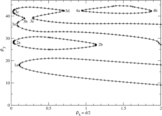
Figure 1: Numerical results for the critical Epstein zeros at small dimensions $d\leq 4$. The critical zeros are connected by solid curves, closed or semi-open, which enclose disjunctive regions of the complex plane. The left and right edge points of the curves are indicated as 1a, 2a, 3a, 3c, 3e, 4a and 2b, 3b, 3d, 4b, respectively.

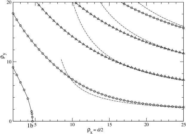
Figure 2: Numerical results for critical Epstein zeros at large dimensions (up to $d=50$). The lowest curve ending up at the edge point 1b corresponds to the prolongation of the lowest curve in Fig. 1. The solid lines of the second (open circles) and third (open triangles) zeros (as they appear in the region of small $d$) go up to $d\to\infty$. The prediction of zeros following from the asymptotic relation (68) is represented by the dashed lines.

From all critical zeros lying on a given curve, the “edge” points, denoted as $\rho^{*}=(d^{*}/2,\rho_{y}^{*})$ with $\rho_{y}^{*}\equiv\rho_{y}(d^{*})$, are the most relevant. They are defined by the tangent ${\rm d}\rho_{y}/{\rm d}d|_{\rho^{*}}=\pm\infty$ or, equivalently, ${\rm d}d/{\rm d}\rho_{y}|_{\rho^{*}}=0$. They satisfy Eq. (24) for the critical zeros, i.e.,

$$-\frac{d^{*}}{\left(\frac{d^{*}}{2}\right)^{2}+{\rho_{y}^{*}}^{2}}+\int_{0}^{1}{\rm d}t\,t^{d^{*}/4-1}\cos\left(\frac{\rho_{y}^{*}\ln t}{2}\right)\left[\theta_{3}^{d^{*}}\left({\rm e}^{-\pi t}\right)-t^{-d^{*}/2}\right]=0,$$ (69)

and simultaneously the derivative of Eq. (24) with respect to $\rho_{y}$, taken with ${\rm d}d/{\rm d}\rho_{y}|_{\rho^{*}}=0$,

$$\frac{2\rho_{y}^{*}d^{*}}{\left[\left(\frac{d^{*}}{2}\right)^{2}+{\rho_{y}^{*}}^{2}\right]^{2}}-\frac{1}{2}\int_{0}^{1}{\rm d}t\,t^{d^{*}/4-1}\sin\left(\frac{\rho_{y}^{*}\ln t}{2}\right)\ln t$$

$$\times\left[\theta_{3}^{d^{*}}\left({\rm e}^{-\pi t}\right)-t^{-d^{*}/2}\right] = 0.$$ (70)

The set of equations (69) and (70) has an infinite number of solutions for $\rho^{*}$ with dimension $d^{*}$ being in general non-integer. We have to distinguish between the “left” edge points, for which ${\rm d}^{2}d/{\rm d}\rho_{y}^{2}|_{\rho^{*}}>0$, and the “right” edge points, for which ${\rm d}^{2}d/{\rm d}\rho_{y}^{2}|_{\rho^{*}}<0$. The coordinates and left/right orientation of edge points in figures 1 and 2 are summarized in Tab. 1.

Table 1: The coordinates and the orientation of the edge points in Figs. 1 and 2.

edge point	orientation	$\rho^{*}_{x}=d^{*}/2$	$\rho^{*}_{y}$
1a	left	0.10846187908294	18.06404476224324
1b	right	4.62277623337280	0
2a	left	0.029260757098957	28.25989865119296
2b	right	1.13615655471973	27.06485479190591
3a	left	0.076684964492103	36.29956597219118
3b	right	0.17608667918405	38.97086173076263
3c	left	0.023788974966443	42.00296457563092
3d	right	0.69958436750509	42.29187347594789
3e	left	0.28286847694364	39.08036320922192
4a	left	0.94484709689530	42.43883096807280
4b	right	1.87159485174678	42.20920217767993

$\rho_{y}$ as the function of $d$ is singular (non-analytic) at the edge points. Let us consider, say, a left edge point with coordinates $(d^{*}/2,\rho_{y}(d^{*}))$ and study an infinitesimal deviation from it along the curve of critical zeros $\rho_{y}(d)$. Setting

$$d=d^{*}+\Delta d\quad(0<\Delta d\ll 1),\quad\rho_{y}(d)=\rho_{y}(d^{*})+\Delta\rho_{y}\quad(\Delta\rho_{y}\ll 1)$$ (71)

in (24) and expanding systematically in powers of small deviations $\Delta d$ and $\Delta\rho_{y}$, one gets

$$\alpha\Delta d+\gamma(\Delta\rho_{y})^{2}-\beta\Delta d\Delta\rho_{y}-\delta(\Delta\rho_{y})^{3}+{\cal O}\left[(\Delta d)^{2}\right]+{\cal O}\left[\Delta d(\Delta\rho_{y})^{2}\right]=0,$$ (72)

where the expansion coefficients are given by

$$\alpha = \frac{\left(\frac{d^{*}}{2}\right)^{2}-{\rho_{y}^{*}}^{2}}{\left[\left(\frac{d^{*}}{2}\right)^{2}+{\rho_{y}^{*}}^{2}\right]^{2}}+\int_{0}^{1}{\rm d}t\,t^{\frac{d^{*}}{4}-1}\cos\left(\frac{\rho_{y}^{*}\ln t}{2}\right)$$ (73)

$$\times\left\{\frac{\ln t}{4}\left[\theta^{d^{*}}_{3}\left({\rm e}^{-\pi t}\right)+t^{-d^{*}/2}\right]+\theta_{3}^{d^{*}}\left({\rm e}^{-\pi t}\right)\ln\left[\theta_{3}\left({\rm e}^{-\pi t}\right)\right]\right\},$$

$$\beta = 2\rho_{y}^{*}\frac{3\left(\frac{d^{*}}{2}\right)^{2}-{\rho_{y}^{*}}^{2}}{\left[\left(\frac{d^{*}}{2}\right)^{2}+{\rho_{y}^{*}}^{2}\right]^{3}}+\frac{1}{2}\int_{0}^{1}{\rm d}t\,t^{\frac{d^{*}}{4}-1}\sin\left(\frac{\rho_{y}^{*}\ln t}{2}\right)\ln t$$ (74)

$$\times\left\{\frac{\ln t}{4}\left[\theta_{3}^{d^{*}}\left({\rm e}^{-\pi t}\right)+t^{-d^{*}/2}\right]+\theta_{3}^{d^{*}}\left({\rm e}^{-\pi t}\right)\ln\left[\theta_{3}\left({\rm e}^{-\pi t}\right)\right]\right\},$$

$$\gamma = d^{*}\frac{\left(\frac{d^{*}}{2}\right)^{2}-3{\rho_{y}^{*}}^{2}}{\left[\left(\frac{d^{*}}{2}\right)^{2}+{\rho_{y}^{*}}^{2}\right]^{3}}-\frac{1}{8}\int_{0}^{1}{\rm d}t\,t^{\frac{d^{*}}{4}-1}\cos\left(\frac{\rho_{y}^{*}\ln t}{2}\right)(\ln t)^{2}$$ (75)

$$\times\left[\theta_{3}^{d^{*}}\left({\rm e}^{-\pi t}\right)-t^{-d^{*}/2}\right],$$

$$\delta = 4d^{*}\rho_{y}^{*}\frac{\left(\frac{d^{*}}{2}\right)^{2}-{\rho_{y}^{*}}^{2}}{\left[\left(\frac{d^{*}}{2}\right)^{2}+{\rho_{y}^{*}}^{2}\right]^{4}}-\frac{1}{48}\int_{0}^{1}{\rm d}t\,t^{\frac{d^{*}}{4}-1}\sin\left(\frac{\rho_{y}^{*}\ln t}{2}\right)(\ln t)^{3}$$ (76)

$$\times\left[\theta_{3}^{d^{*}}\left({\rm e}^{-\pi t}\right)-t^{-d^{*}/2}\right].$$

Note that the linear term of order $\Delta\rho_{y}$ is missing in (72) due to the validity of Eq. (70) for the critical edge zeros.

For $d>d^{*}$ $(\Delta d>0)$, Eq. (72) tells us that the leading order of the expansion of $\Delta\rho_{y}$ with respect to $\Delta d$ is given by the relation $\alpha\Delta d+\gamma(\Delta\rho_{y})^{2}=0$, i.e.,

$$\Delta\rho_{y}\sim\pm\sqrt{-\frac{\alpha}{\gamma}}\sqrt{\Delta d},$$ (77)

where the prefactor sign $\pm$ specifies the up and down branches of the plot $\rho_{y}(d)$. Notice that $-\alpha/\gamma$ must be a positive number to get a real solution for $\rho_{y}(d)$ and our numerical calculations confirm that for all studied left edge points it really is so. Singular relations of type (77) with exponent $\frac{1}{2}$ occur also for the order parameter in critical phenomena of statistical systems at the second-order phase transition within the so-called mean-field approach [57, 58]. The next order of the expansion of $\Delta\rho_{y}$ in $\Delta d$ follows from Eq. (72) by considering two additional terms of the order $(\Delta d)^{3/2}$. Adding a term $c\Delta d$ to the formula for $\Delta\rho_{y}$ in (77) and expanding all functions up to the order $(\Delta d)^{3/2}$ fixes $c$ as follows $2\gamma c=\beta-\alpha\delta/\gamma$. We conclude that

$$\rho_{y}(d) = \rho_{y}(d^{*})\pm\sqrt{-\frac{\alpha}{\gamma}}\sqrt{d-d^{*}}+\frac{1}{2\gamma}\left(\beta-\frac{\alpha\delta}{\gamma}\right)(d-d^{*})$$ (78)

$$+{\cal O}\left[(d-d^{*})^{3/2}\right].$$

A similar analysis can be made for right edge zeros.

6 Generation of off-critical zeros from critical edge zeros

This section is about a continuous generation of off-critical zeros from the critical edge zeros.

In the case of the left edge zero, Eq. (72) with $-\alpha/\gamma>0$ has no real solution for $\Delta\rho_{y}$ if $\Delta d=d-d^{*}<0$. Let us assume that for $\Delta d<0$ there is also a continuous deviation of the $\rho_{x}$-component from its critical value $\frac{d}{2}$, see Eq. (25). Considering then the relations (71) in equations (26) and (27) and expanding in powers of small variables $\Delta d$, $\Delta\rho_{x}$ and $\Delta\rho_{y}$, one obtains

$$\alpha\Delta d-\gamma(\Delta\rho_{x})^{2}+\gamma(\Delta\rho_{y})^{2}-\beta\Delta d\Delta\rho_{y}+3\delta(\Delta\rho_{x})^{2}\Delta\rho_{y}$$

$$-\delta(\Delta\rho_{y})^{3}+\cdots = 0,$$ (79)

$$\Delta\rho_{x}\left[\beta\Delta d-2\gamma\Delta\rho_{y}-\delta(\Delta\rho_{x})^{2}+3\delta(\Delta\rho_{y})^{2}+\cdots\right] = 0.$$ (80)

As is evident from the first relation (79), setting $\Delta\rho_{x}=0$, $\Delta\rho_{y}$, which is real for $\Delta d>0$, becomes pure imaginary for $\Delta d<0$ (in the leading order of its expansion in $\Delta d$) which is in contradiction with the definition of $\rho_{y}$ as a real number. However, the term $\gamma(\Delta\rho_{y})^{2}$ containing the variable $\Delta\rho_{y}$ has a counterpart with the opposite sign $-\gamma(\Delta\rho_{x})^{2}$ containing the variable $\Delta\rho_{x}$ as the actual candidate for the leading-order symmetry breaking $\Delta\rho_{x}\neq 0$. In the leading order, the equation $\alpha\Delta d-\gamma(\Delta\rho_{x})^{2}=0$ implies that

$$\Delta\rho_{x}\sim\pm\sqrt{-\frac{\alpha}{\gamma}}\sqrt{-\Delta d},$$ (81)

where the $\pm$ sign reflects the split of $\Delta\rho_{x}$ onto two different branches (see discussion below). Since $\Delta\rho_{x}\neq 0$, the second relation (80) implies that the leading order is determined for $\Delta\rho_{y}$ by $\beta\Delta d-2\gamma\Delta\rho_{y}-\delta(\Delta\rho_{x})^{2}=0$, i.e.,

$$\Delta\rho_{y}=-\frac{1}{2\gamma}\left(\beta-\frac{\alpha\delta}{\gamma}\right)(d^{*}-d)+{\cal O}\left[(d^{*}-d)^{3/2}\right],\qquad d<d^{*}.$$ (82)

The next order of the expansion of $\Delta\rho_{x}$ in $-\Delta d$ follows from Eq. (79) by adding a term $c(-\Delta d)$ to the formula for $\Delta\rho_{x}$ in (81). The term arising from $(\Delta\rho_{x})^{2}$, which is proportional to $c(-\Delta d)^{3/2}$, has no counterparts since all additional terms in (79) are of the order $(-\Delta d)^{2}$. Consequently, $c=0$ and one gets

$$\Delta\rho_{x}=\pm\sqrt{-\frac{\alpha}{\gamma}}\sqrt{d^{*}-d}+{\cal O}\left[(d^{*}-d)^{3/2}\right],\qquad d<d^{*}.$$ (83)

We conclude that the expansion of up and down branches of $\rho_{y}(d)$ (78), valid for $d>d^{*}$, splits into the expansion for the left and right branches (tails) (83) and (82), valid for $d<d^{*}$, with similar expansion coefficients. While the previous two up and down branches of $\rho_{y}(d)$ for $d>d^{*}$ were not bound by a symmetry, the positive and negative branches of off-critical zeros $[\rho_{x}(d),\rho_{y}(d)]$ for $d<d^{*}$ are bound by the symmetry $[\rho_{x}(d),\rho_{y}(d)]\to[d-\rho_{x}(d),\rho_{y}(d)]$ which takes place for every deviation from the edge point. A similar analysis can be made for right edge zeros, to keep the parameter $\Delta d$ negative from the side of off-critical zeros it must be defined as $\Delta d=d^{*}-d$.

The numerical evaluation of off-critical zeros using Mathematica is relatively simple due to the continuity of tails as $d$ starts to deviate from $d^{*}$. As the function to deal with, one takes the sum of two squares of the lhs of equations (26) and (27) which should vanish at zeros. The command FindMinimum is applied to the function and the zero is taken as guaranteed if the function value is of order at most $10^{-23}$. To prevent escape from the local minimum, one starts from (say right) edge point by shifting the dimension by a tiny amount 0.0001, after few steps the shift can be increased to 0.001 and finally to 0.01. To find a minimum takes approximately 60 seconds of CPU time on a standard PC.

In what follows, various scenarios are presented how the two conjugate tails of off-critical zeros behave during their $d$-evolution.

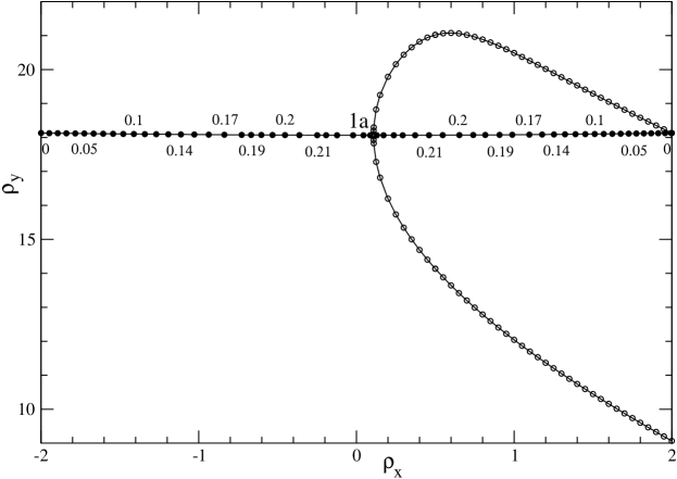
Figure 3: The left and right tails of off-critical zeros (full circles) starting from the critical edge point 1a $(d^{*}\approx 0.217)$. The dimension of off-critical zeros is indicated at a few points. The tails go down to $d=0$ at the points $(\pm 2,4\pi/\ln 2)$.

The simplest scenario, presented in Fig. 3, is associated with the left edge point denoted as 1a in Fig. 1. The critical zeros are represented by open circles, the left and right tails of off-critical zeros by full circles. The dimension of off-critical zeros is indicated at a few points. The left and right tails of off-critical zeros start from $d^{*}\approx 0.217$ at the edge point 1a and go down monotonously to $d=0$ at points $(-2,4\pi/\ln 2)$ and $(2,4\pi/\ln 2)$, respectively. The latter points coincide with the $k=1$ zeros (53) found in $d=0$. As is seen in the figure, the end-point of the right tail $(2,4\pi/\ln 2)$ coincides with a critical zero at $d=4$.

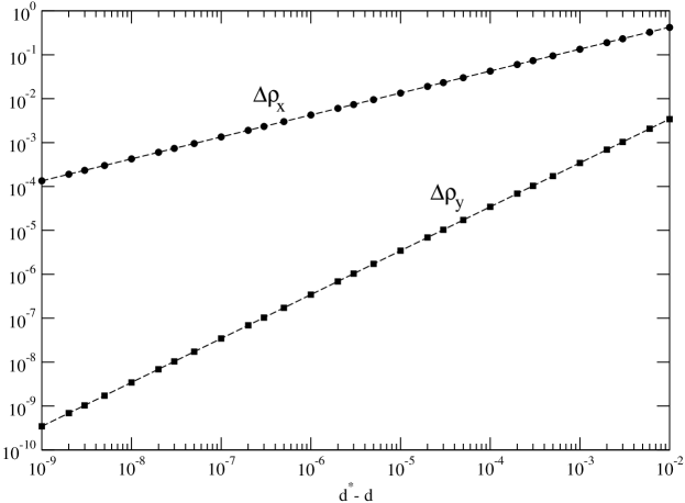
Figure 4: The log-log plot of numerical data for the dependence of $\Delta\rho_{x}$ (full circles) and $\Delta\rho_{y}$ (full squares) on the small dimension deviation $d^{*}-d$ for the right tail going from the left edge point 1a. Data fit perfectly with the analytic predictions (84) represented in logarithmic scale by the dashed straight lines.

The test of the expansion formulas (82) and (83) for the right tail generated from the left edge point 1a is presented in Fig. 4. Our numerical data for the dependence of $\Delta\rho_{x}$ and $\Delta\rho_{y}$ on $d^{*}-d$ are represented in logarithmic scale by full circles and squares, respectively. For small deviations from the edge point $d^{*}-d\to 0^{+}$, the expansion formulas (82) and (83), with the constants $\alpha,\beta,\gamma,\delta$ evaluated by using the formulas (73)-(76), lead to

$$\Delta\rho_{x}\sim\pm 4.24563\sqrt{d^{*}-d},\qquad\Delta\rho_{y}\sim 0.344516(d^{*}-d).$$ (84)

The log-log plots of these analytic predictions, represented in Fig. 4 by the dashed straight lines, fit perfectly the corresponding numerical data for the small deviation $d^{*}-d$ ranging from $10^{-9}$ to $10^{-2}$.

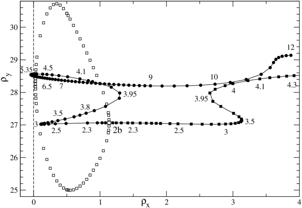
Figure 5: The left (full circles) and right (full squares) tails of off-critical zeros starting from the critical edge point 2b $(d^{*}\approx 2.272)$. Dimension $d$ increases along the tails up to $\infty$, only fragments of the tails are shown in the figure.

The form of the tails of off-critical zeros is more complicated in the case of the right edge point 2b (as denoted in Fig. 1), see Fig. 5. Because of the right orientation of this edge point, dimension $d$ increases along the left (full circles) and right (full squares) tails from $d^{*}\approx 2.272$ to $\infty$. As a check, for the left tail we recover a special off-critical zero which occurs simultaneously in dimensions $d=4$ and $d=8$, see equations (5) and (7), and coincide with the fourth critical zero of the $d=2$ Epstein zeta-function. For the dimension of special physical interest $d=3$, the left tail contains the off-critical zero $\rho\approx 0.111189793551259+27.0278811412527548{\rm i}$. It is interesting that the left tail covers also a tiny interval of negative values of $\rho_{x}$ for dimensions from the interval $[4.965,5.775]$. This means that for integer dimension $d=5$ there exists a pair of conjugate off-critical zeros with the same imaginary component, namely $\rho_{y}\approx 28.5599914110240345$, and the real components $\rho_{x}\approx-0.00717997528701,5.00717997528701$ which lie outside the critical strip $[0,5]$. This phenomenon is usually present in lower dimensions with critical strips of small width, especially for $d$ between 0 and 1, see Figs. 3 and 6.

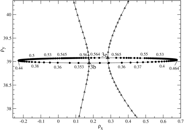
Figure 6: Interpolation of off-critical zeros (full circles) between the right edge point 3b $(d^{*}\approx 0.352)$ and the left edge point 3e $(d^{*}\approx 0.566)$, both edge points lying on the same curve of critical zeros (open triangles).

Another scenario is presented in Fig. 6 where the two tails of off-critical zeros (full circles) interpolate between the right edge point 3b $(d^{*}\approx 0.352)$ and the left edge point 3e $(d^{*}\approx 0.566)$, both points lying on the same curve of critical zeros (open triangles). Although the interval of dimensions is relatively narrow, the interval of $\rho_{x}$-values of off-critical zeros is relatively large and involves also negative values.

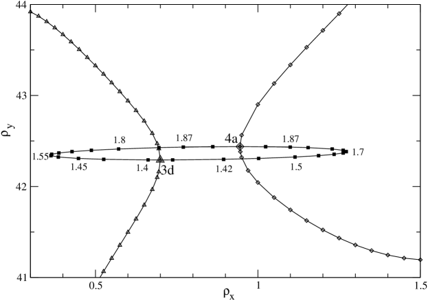
Figure 7: Interpolation of off-critical zeros (full squares) between the right edge point 3d $(d^{*}\approx 1.399)$ and the left edge point 4a $(d^{*}\approx 1.890)$, the edge points lying on distinct curves of critical zeros (open triangles and diamonds).

In Fig. 7, the two tails of off-critical zeros (full squares) interpolate between the right edge point 3d $(d^{*}\approx 1.399)$ and the left edge point 4a $(d^{*}\approx 1.890)$ which lie on different curves of critical zeros (open triangles and diamonds).

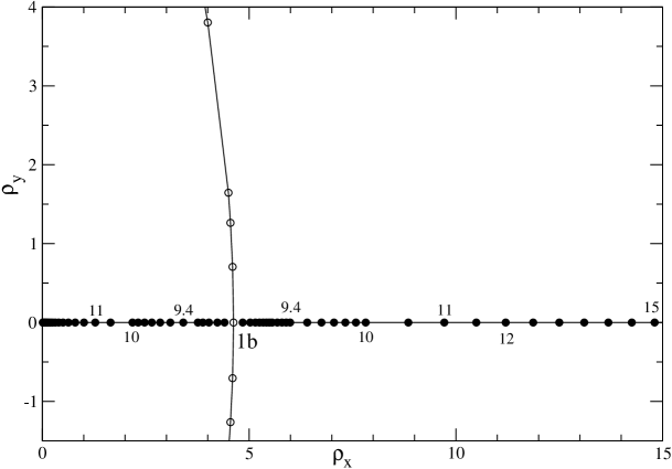
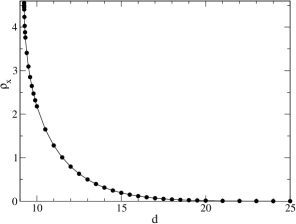
Figure 8: Two conjugate tails of the real off-critical zeros (full circles) coming from the right edge point 1b $(d^{*}\approx 9.24555)$, localized at the intersection of the curve of critical zeros (open circles) and the real axis. The dimension of off-critical zeros is indicated at a few points. The inset describes the quick approach of the numerical values of $\rho_{x}$ (full circles) to zero when increasing dimension $d$.

The critical point 1b in Fig. 2 is a right edge point because the curve continues reflection-symmetrically across the $\rho_{x}$-axis into the lower quadrant. The position of this point $({\rho_{c}^{*}})_{x}=d_{c}^{*}/2$ can be found by setting $\rho_{y}=0$ in (24),

$$-\frac{4}{d_{c}^{*}}+\int_{0}^{1}{\rm d}t\,t^{d_{c}^{*}/4-1}\left[\theta_{3}^{d_{c}^{*}}\left({\rm e}^{-\pi t}\right)-t^{-d^{*}_{c}/2}\right]=0.$$ (85)

The numerical solution of this equation is $d_{c}^{*}=9.24555\ldots$. For every $d>d_{c}^{*}$, there exists a pair of off-critical zeros on the real axis [note that Eq. (27) holds automatically for $\rho_{y}=0$] whose conjugate components $\rho_{x}$ and $d-\rho_{x}$ satisfy the integral equation

$$-\frac{1}{\rho_{x}}-\frac{1}{d-\rho_{x}}+\int_{0}^{1}\frac{{\rm d}t}{t}\frac{t^{\rho_{x}/2}+t^{(d-\rho_{x})/2}}{2}\left[\theta_{3}^{d}\left({\rm e}^{-\pi t}\right)-t^{-d/2}\right]=0.$$ (86)

The two solutions of this equation are lying in the critical strip $0<\rho_{x}<d$, see Fig. 8. This can be explained for integral dimensions $d$ by the fact that for real $\rho>d$ the Epstein zeta-function is the sum of positive numbers and therefore cannot vanish. To be more particular, for $d=10$ one has the pair of real zeros $\rho=2.17985543147...;7.82014456853...$, for $d=12$ one has $\rho=0.7951625733...;11.2048374267...$, for $d=20$ one has $\rho=0.0127182144...;19.9872817856...$, etc. In the large-$d$ limit, the two solutions tend to the boundaries $0$ and $d$ of the critical strip. The quick approach to 0 of the numerical values of $\rho_{x}$ (full circles) is presented in the inset of Fig. 8.

7 Conclusion

The basic definition of the hypercubic Epstein zeta-function (2) requires an integer value of the spatial dimension $d$. The analytic continuation of the lattice sum to the whole complex $s$-plane (15) is well defined also for non-integer values of $d$. This extension was used to obtain numerically the closed or semi-open curves $\rho_{y}(d)$ of critical zeros (on the critical line), see figures 1 and 2. Each curve involves a finite number of left/right critical edge points $\rho^{*}=(d^{*}/2,\rho_{y}(d^{*}))$, defined by an infinite tangent ${\rm d}\rho_{y}/{\rm d}d|_{\rho^{*}}$. The coordinate data in Tab. 1 indicate that the dimension of edge critical points is in general non-integer. As was shown in section 5, the function $\rho_{y}(d)$ is a singular function of the dimension deviation $d-d^{*}>0$ $(d^{*}-d>0)$ for the left (right) edge points. Changing the sign of the dimension deviation to $d-d^{*}<0$ $(d^{*}-d<0)$ for the left (right) edge points, these edge points give rise to two conjugate tails of off-critical zeros (off the critical line) with continuously varying dimension $d$, in formal analogy with critical phenomena for many-body statistical systems (section 6). Various versions of the generation mechanism are presented. Fig. 3 documents the generation of the left and right tails of off-critical zeros from the left edge point 1a $(d^{*}\approx 0.217)$, the dimension along the tails goes down to $0$ at the off-critical zeros $(\pm 2,4\pi/\ln 2)$. The corresponding log-log plots of numerical data for $\Delta\rho_{x}(d)=\rho_{x}(d)-\frac{d^{*}}{2}$ and $\Delta\rho_{y}(d)=\rho_{y}(d)-\rho_{y}(d^{*})$ in the case of the right tail, presented in Fig. 4, are in perfect agreement with the analytic prediction (84) valid for small dimension deviations $d^{*}-d$. The generation of the off-critical tails from the right edge point 2b, with dimension along tails going up to infinity, is pictured in Fig. 5. The interpolation of off-critical zeros between the right edge point 3b and the left edge point 3e, both edge points lying on the same curve of critical zeros, is presented in Fig. 6. Fig. 7 concerns an interpolation of off-critical zeros between the right edge point 3d and the left edge point 4a, the edge points lying on different curves of critical zeros. For every $d>d^{*}_{c}\approx 9.246$, there exists a pair of conjugate off-critical zeros on the real axis, having their origin in the right edge point 1b, see Fig. 8. As $d\to\infty$, the two zeros tend very quickly to the boundaries $0$ and $d$ of the critical strip.

As a by-product of the formalism, we have derived the exact formula (52) for $\lim_{d\to 0^{+}}\zeta^{(d)}(s)/d$. This formula tells us that there are no critical zeros in the limit $d\to 0^{+}$. In the studied interval of $\rho_{y}$-values smaller than 45, there is always a finite gap between the axis $\rho_{x}=0$ and the smallest $\rho_{x}$-component of the critical zeros; a remaining open question is whether a non-zero gap is present for all critical zeros (with larger values of $\rho_{y}$). The spectrum of off-critical zeros in the limit $d\to 0^{+}$ was checked to fulfill the obligatory sum rules. Another check of the spectrum is that off-critical tails generated from the left edge points end correctly at the $d\to 0^{+}$ off-critical zeros. The exact treatment of the large-$d$ limit in section 4.2 predicts an equidistant distribution of the critical zeros along the imaginary axis (68). This result is confirmed numerically in Fig. 2 where the critical zeros (open circles, triangles and squares) approach to for sufficiently large $d$ the equidistant distribution (68) represented by the dashed lines.

Another open question is whether the presented mechanism of generation of the tails of off-critical zeros from the critical edge points is the only one. We anticipate that it is so.

References

- [1] J.S. Brauchart, Optimal Discrete Riesz energy and discrepancy, Unif. Distrib. Theory 6 (2011) 207–220.
- [2] B. Riemann, Über die Anzahl der Primzahlen unter einer gegebenen Grösse. Monats-berichte der Berliner Akademie (1859) 671–680.
- [3] G.H. Hardy, Sur les zeros de la fonction , Compt. Rend. Acad. Sci. 158 (1914) 1012–-1014.
- [4] M. Riesz, Sur l’hypothèse de Riemann, Acta Math. 40 (1916) 185–-190.
- [5] G.H. Hardy, J.E. Littlewood, The zeros of Riemann’s zeta-function on the critical line, Math. Z. 10 (1921) 283–317.
- [6] J.I. Hutchinson, On the Roots of the Riemann Zeta-Function. Trans. Amer. Math. Soc. 27 (1925) 49–60.
- [7] E.C. Titchmarsh, The Zeros of the Riemann Zeta-Function, Proc. Royal Soc. London A 151 (1935) 234–255.
- [8] A. Selberg, Contributions to the theory of the Riemann zeta-function, Arch. Math. Naturvid. 48 (1946) 89–-155.
- [9] H.M. Edwards, Riemann’s Zeta Function, Dover Publications, New York, 1974.
- [10] A. Ivić, The Riemann Zeta Function, John Wiley & Sons, New York, 1985.
- [11] E.C. Titchmarsh, The Theory of The Riemann Zeta-function, 2nd ed., Clarendon Press, Oxford, 1988.
- [12] E.W. Barnes, On the theory of the multiple gamma function, Trans. Camb. Philos. Soc. 19 (1904) 374–-425.
- [13] P. Epstein, Zur Theorie allgemeiner Zetafunctionen, Math. Ann. 56 (1903) 615–644.
- [14] P. Epstein, Zur Theorie allgemeiner Zetafunctionen II, Math. Ann. 63 (1907) 205–216.
- [15] T.M. Apostol, Introduction to Analytic Number Theory, Springer Verlag, Berlin, 1976.
- [16] T.M. Apostol, Modular function and Dirichlet series in number theory, Springer Verlag, Berlin, 1990.
- [17] J.M. Borwein, M.L. Glasser, R.C. McPhedran, J.G. Wan, J.L. Zucker, Lattice Sums Then and Now, Cambridge University Press, Cambridge, 2013.
- [18] D. Ruelle, Dynamical zeta functions and transfer operators, Notices Amer. Math. Soc. 49 (2002) 887–895.
- [19] E. Elizalde, S.D. Odintsov, A. Romeo, S. Zerbini, Zeta Regularization Techniques With Applications, World Scientific, Singapore, 1994.
- [20] K.A. Milton, The Casimir Effect: Physical Manifestations of Zero-point Energy, World Scientific, River Edge, 2001.
- [21] A. Edery, Multidimensional cut-off technique, odd-dimensional Epstein zeta-functions and Casimir energy of massless scalar fields, J. Phys. A: Math. Gen. 39 (2006) 685–712.
- [22] F. Dalvovo, O. Giorgini, L. Pitaevskii, S. Stringari, Theory of Bose-Einstein condensation in trapped gases, Rev. Mod. Phys. 71 (1999) 463–512.
- [23] K. Kirsten, F.L. Williams, A Window into Zeta and Modular Physics, Cambridge University Press, Cambridge, 2010.
- [24] E. Elizalde, Ten Physical Applications of Spectral Zeta Functions, Springer Verlag, Berlin, 2012.
- [25] S. Chowla, A. Selberg, On Epstein’s zeta function, Proc. Natl. Acad. Sci. USA 35 (1949) 371–374.
- [26] V. Ennola, On a problem about the Epstein zeta function. Proc. Camb. Philos. Soc. 60 (1964) 855–875.
- [27] E. Elizalde, A. Romeo, Regularization of general multidimensional Epstein Zeta-functions, Rev. Math. Phys. 1 (1989) 113–128.
- [28] X. Blanc, M. Lewin, The crystallization conjecture: a review, EMS Surveys Math. Sci. 2 (2015) 255–306.
- [29] M.L. Glasser, The evaluation of lattice sums. I. Analytic procedures, J. Math. Phys. 14 (1973) 409–413.
- [30] M.L. Glasser, The evaluation of lattice sums. II. Number-theoretic approach, J. Math. Phys. 14 (1973) 701–703.
- [31] I.J. Zucker, Exact results for some lattice sums in 2, 4, 6 and 8 dimensions, J. Phys. A: Math. Nucl. Gen. 7 (1974) 1568–1575.
- [32] D. Borwein, J.M. Borwein, A. Straub, On lattice sums and Wigner limits, J. Math. Anal. Appl. 414 (2014) 489–513.
- [33] L. Lorenz, Bidrag til talenes theori, Tidsskr. Fur. Math. 1 (1871) 97–114.
- [34] G.H. Hardy, Notes on some points in the integral calculus LII: On some definite integrals considered by Mellin, Messenger Math. 49 (1920) 85–91.
- [35] A. Lander, The Zeros of the Dirichlet beta function encode the odd primes and have real part 1/2, Preprints 2018, 2018040305 (doi: 10.20944/preprints201804.0305.v1)
- [36] D.A. Hejhal, Zeros of Epstein zeta functions and supercomputers, Proceedings of the International Conference of Mathematicans, Berkeley, California, USA, 1986, 1362–1384.
- [37] E. Bogomolny, P. Leboeuf, Statistical properties of the zeros of zeta functions - beyond the Riemann case, Nonlinearity 7 (1994) 1155–1167.
- [38] H.S.A. Potter, E.C. Titchmarsh, The zeros of Epstein’s zeta functions, Proc. London Math. Soc. 39 (1935) 372–384.
- [39] H. Davenport, H. Heilbronn, On the zeros of certain Dirichlet series I, II, J. London Math. Soc. 11 (1936) 181–185 and 307–312.
- [40] P.T. Bateman, E. Grosswald, On Epstein’s zeta function, Acta Arithmetica, 9 (1964) 365–373.
- [41] H.M. Stark, On the zeros of Epstein’s zeta function. Mathematika 14 (1967) 47–55.
- [42] R.C. McPhedran, Zeros of lattice sums: 1. Zeros of the critical line, arXiv:1601.01724 (2016).
- [43] M. Jutila, K. Srinivas, Gaps between the zeros of Epstein’s zeta-functions on the critical line, Bull. London Math. Soc. 37 (2005) 45–53.
- [44] S. Baier, K. Srinivas, U.K. Sangale, A note on the gaps between zeros of Epstein’s zeta-functions on the critical line, Funct. Approx. Comment. Math. 57 (2017) 235–253.
- [45] E. Elizalde, Multiple zeta functions with arbitrary exponents, J. Phys. A: Math. Gen. 22 (1989) 931–942.
- [46] K. Kirsten, Generalized multidimensional Epstein zeta functions, J. Math. Phys. 35 (1994) 459–470.
- [47] G.S. Joyce, On the Laurent series for the Epstein zeta function, J. Phys. A: Math. Theor. 49 (2016) 405204.
- [48] R.A. Rankin, A minimum problem for the Epstein zeta function, Proc. Glasg. Math. Assoc. 1 (1953) 149–158.
- [49] J.W.S. Cassels, On a problem of Rankin about the Epstein function, Proc. Glasg. Math. Assoc. 4 (1959) 73–80.
- [50] P.H. Diananda, Notes on two lemmas concerning the Epstein zeta-function, Proc. Glasg. Math. Assoc. 6 (1964) 202–204.
- [51] P. Sarnak, A. Strömbergsson, Minima of Epstein’s zeta function and heights of flat tori, Invent. Math. 165 (2006) 115–151.
- [52] S.C. Lim, L.P. Teo, On the minima and convexity of Epstein zeta function, J. Math. Phys. 49 (2008) 073513.
- [53] E. Bombieri, D.A. Hejhal, On the zeros of Epstein zeta-functions, C.R. Acad. Sci. Paris Sér. I Math. 304 (1987) 213–-217.
- [54] J. Steuding, On the zero-distribution of Epstein zeta-functions, Math. Ann. 333 (2005) 689–697.
- [55] T. Nakamura, L. Pankowski, On zeros and c-values of Epstein zeta-functions, Šiauliai Math. Semin. 8 (2013) 181–195.
- [56] R.E. Crandall, Fast evaluation of multiple zeta sums, Math. Comp. 67 (1998) 1163–1172.
- [57] R.J. Baxter, Exactly Solved Models in Statistical Mechanics, Academic Press, London, 1982.
- [58] L. Šamaj, Z. Bajnok, Introduction to the Statistical Physics of Integrable Many-body Systems, Cambridge University Press, Cambridge, 2013.
- [59] I.S. Gradshteyn, I.M. Ryzhik, Table of Integrals, Series, and Products, 6th edn., Academic Press, London, 2000.
- [60] A. Terras, The minima of quadratic forms and the behavior of Epstein and Dedekind zeta functions, J. Number Theory 12 (1980) 258–272.
- [61] L. Šamaj, E. Trizac, Critical phenomena and phase sequence in a classic bilayer Wigner crystal at zero temperature, Phys. Rev. B 85 (2012) 205131.
- [62] E.T. Whittacker, G.N. Watson, A Course of Modern Analysis, Cambridge University Press, Cambridge, 1996.
- [63] R.C. McPhedran, Sum rules for functions of the Riemann zeta type, arXiv:1801.07415 (2018).
- [64] J. Hadamard, Étude sur les propriétés des fonction entières et un particulier d’une fonction considéré par Riemann, J. Math. Pure Appl. 9 (1893) 171–215.
- [65] D.H. Lehmer, The sum of like powers of the Riemann zeta function, Math. Comp. 50 (1988) 265–273.
- [66] J.B. Keiper, Power series expansions of Riemann’s function, Math. Comp. 58 (1992) 765–773.
- [67] X.J. Li, The positivity of a sequence of numbers and the Riemann hypothesis, J. Number Th. 65 (1997) 325–333.
- [68] S.R. Finch, Mathematical constants, Cambridge University Press, Cambridge, 2003.
- [69] M.W. Coffey, New summation relations for the Stieltjes constants, Proc. R. Soc. A 462 (2006) 2563–2573.