Universal scaling of three-dimensional dimerized quantum antiferromagnets on bipartite lattices

Abstract

Using the first principles quantum Monte Carlo (QMC) calculations, we investigate the previously established universal scaling between the Néel temperature $T_{N}$ and the staggered magnetization density $M_{s}$ of three-dimensional (3D) dimerized quantum antiferromagnets. Particularly, the calculations are done on both the stacked honeycomb and the cubic lattices. In addition to simulating models with two types of antiferromagnetic couplings (bonds) like those examined in earlier studies, here a tunable parameter controlling the strength of third type of bond is introduced. Interestingly, while the data of models with two types of bonds obtained here fall on top of the universal scaling curves determined previously, the effects due to microscopic details do appear. Moreover, the most striking result suggested in our study is that with the presence of three kinds of bonds in the investigated models, the considered scaling relations between $T_{N}$ and $M_{s}$ can be classified by the coordinate number of the underlying lattice geometries. The findings presented here broaden the applicability of the associated classification schemes formerly discovered. In particular, these results are not only interesting from a theoretical point of view, but also can serve as useful guidelines for the relevant experiments.

I Introduction

Finding relations among quantities which are universal, namely being valid for various systems is a fascinating task in the physical world. Moreover, to be able to classify these relations are crucial and important considering its great potential applications in the relevant experiments. The critical exponents of second order phase transitions is one of such examples Nig92 ; Car10 ; Sac11 . For instance, for three-dimensional (3D) classical Heisenberg model and any two-dimensional (2D) dimerized quantum spin systems, when the relevant phase transitions occur in these systems, their associated critical exponents all have the same numerical values Cam02 ; Pel02 . Because these models have either $O(3)$ or $SU(2)$ symmetry, this universality class is called the $O(3)$ universality class in the literature. Other models having different symmetries and dimensions, such as 3D Ising model or 2D classical XY model, belong to various universality classes. Apart from phase transitions, universal quantities associated with quantum critical regime (QCR) is yet another well-known example as well Chu93 ; Chu931 ; Chu94 ; San95 ; Tro96 ; Tro97 ; Tro98 ; Kim00 ; Sen15 ; Tan182 . To conclude, the concept of universality does play a dominated role in many fields of physics.

Recently, experimental results of TlCuCl₃ Rue03 ; Rue08 ; Mer14 have inspired several studies of the 3D dimerized spin-1/2 Heisenberg models Kul11 ; Oit12 ; Jin12 ; Kao13 ; Yan15 ; Har15 ; Tan15 ; Har17 ; Har171 ; Tan17 ; Har172 ; Tan181 . In particular, these theoretical investigations have focused on three universal scaling relations between the Néel temperature $T_{N}$ and the staggered magnetization density $M_{s}$. Two of them, namely $T_{N}/\overline{J}$ versus $M_{s}$ and $T_{N}/T^{\star}$ against $M_{s}$ will be the main topics presented in this study. The $\overline{J}$ and $T^{\star}$ appearing above are the summation of antiferromagnetic couplings connecting to a spin and the temperature $T$ at which the uniform susceptibility $\chi_{u}$ take its maximum value, respectively.

The universal scaling between $T_{N}/\overline{J}$ ($T_{N}/T^{\star}$) and $M_{s}$ is firstly demonstrated in Ref. Jin12 . Particularly the models considered in Ref. Jin12 has the property that each spin is touched by one antiferromagnetic coupling which has larger magnitude than the rest attaching to the same spin (The antiferromagnetic couplings will be called bonds whenever no confusion arises). Extending the work of Ref. Jin12 , classification schemes for both the scaling relations are established in Ref. Tan181 . Specifically, the scaling relations between $T_{N}$ and $M_{s}$ mentioned above can be categorized by the number of strong bonds emerging from each spin.

It is interesting to notice that in Refs. Jin12 ; Tan181 , all the considered models have two kinds of bonds only. Moreover, the investigations are carried out on cubic and double-cubic lattices which are in a sense both of the same type in geometry. As a result, it will be interesting to examine whether the found classification schemes are valid for other kinds of lattice geometries, and when additional (spatially) anisotropic parameters are introduced into the systems.

Due these intriguing motivations described above, here using the quantum Monte Carlo (QMC) simulations, we have studied these two scaling relations of $T_{N}$ and $M_{s}$ on both the stacked honeycomb and the cubic lattices. Furthermore, a tunable parameter is taken into account in our investigation so that the studied quantum spin systems with three types of antiferromagnetic bonds can arise.

While as one expects that the data determined from models with two kinds of bonds on the stacked honeycomb lattice do fall on top of the universal curves obtained in Ref. Tan181 , mild effects because of the microscopic details appear. In addition, our results strongly suggest that a yet to be discovered rule exists since some outcomes from two different lattice geometries collapse smoothly to form a curve. Finally, the most compelling observation implying here is that with the presence of the new (anisotropic) parameter, the two scaling relations studied in this investigation can be categorized by the coordinate number of the underlying lattices (This will be explained in detail later). This new rule can be treated as a very useful supplement to the ones found in Ref. Tan181

The rest of this paper is organized as follows. After the introduction, the models as well as the relevant observable are introduced. Following that we present our results. In particular the numerical evidences for the new classification rules mentioned above are demonstrated. Finally, a section concludes our study.

II Microscopic models and observables

The Hamiltonian of the studied 3D spin-1/2 dimerized antiferromagnets on the stacked honeycomb and the cubic lattices is generally given by

$$H = \sum_{\langle ij\rangle}J_{ij}\,\vec{S}_{i}\cdot\vec{S}_{j}+\sum_{\langle i^{\prime}j^{\prime}\rangle}\alpha_{i^{\prime},j^{\prime}}J^{\prime}_{i^{\prime}j^{\prime}}\,\vec{S}_{i^{\prime}}\cdot\vec{S}_{j^{\prime}},$$ (1)

where in Eq. (1) $J_{ij}$ and $J^{\prime}_{i^{\prime}j^{\prime}}$ are the antiferromagnetic couplings (bonds) connecting nearest neighbor spins $\langle ij\rangle$ and $\langle i^{\prime}j^{\prime}\rangle$ located at sites of the considered 3D lattices, respectively. In addition, for each pair of ${i^{\prime},j^{\prime}}$ the associated anisotropic factor $\alpha_{i^{\prime}j^{\prime}}$ satisfies $0<\alpha_{i^{\prime}j^{\prime}}\leq 1$. Finally, $\vec{S}_{i}$ is the spin-1/2 operator at site $i$. In this study, for any site pairs ${i^{\prime}j^{\prime}}$ and ${ij}$, we have set $J_{ij}=1$ and use the convention $J^{\prime}_{i^{\prime}j^{\prime}}>J_{i,j}$. Figure 1 demonstrates the bond arrangement in the $x$-$y$ plane of the dimerized spin-1/2 models studied here. Moreover, for all the considered systems, in the $z$-direction one has only $J$ and $J^{\prime}$ bonds and they are always set up alternately. From fig. 1 as well as the associated caption, one finds that each spin of the studied models is connected to antiferromagnetic couplings of either two or three kinds of strength. With the conventions employed here, for each model the targeted quantum phase transition is induced by tuning the ratio $J^{\prime}/J$.

   

   

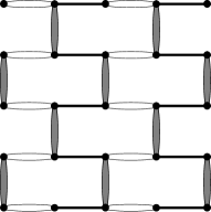
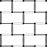
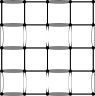
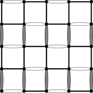
Figure 1: The bond arrangement in the $x$-$y$ plane of the 3D dimerized spin-1/2 Heisenberg models on the stacked honeycomb and the cubic lattices investigated here. The filled and empty ovals, as well as the thin line represent the bonds with antiferromagnetic couplings $J^{\prime}$, $\alpha J^{\prime}$ and $J$, respectively. Here $0<\alpha\leq 1$. For all the considered models, in the $z$-direction one has only $J$ and $J^{\prime}$ bonds and they are always set up alternately. Model on the stacked honeycomb lattice with each spin touching two strong bonds is obtained by letting $J_{2}=J^{\prime}$ and $J_{1}=J$ for these bonds in each $x$-$y$ plane. The model of the left top and bottom panels are called the stair and meander models here, respectively.

To carry out the proposed investigation, particularly to calculate $T_{N}$, $M_{s}$, as well as $T^{\star}$ of the considered dimerized systems, several observables including the staggered structure factor $S(\pi,\pi,L)$ on a finite lattice with linear size $L$ boxsize , both the spatial and temporal winding numbers squared ($\langle W_{i}^{2}\rangle$ for $i\in\{1,2,3\}$ and $\langle W_{t}^{2}\rangle$), spin stiffness $\rho_{s}$, first Binder ratio $Q_{1}$, and second Binder ratio $Q_{2}$ are measured. The definitions of these physical quantities as well as how they can be recorded in the associated Monte Carlo simulations are well known and are available in numerous relevant publications, see Ref. San97 for a detailed introduction.

The staggered structure factor $S(\pi,\pi,\pi,L)$, which is relevant for the determination of $M_{s}$, is defined by

$$S(\pi,\pi,\pi,L)=3\langle(m_{s}^{z})^{2}\rangle,$$ (2)

where $m_{s}^{z}=\frac{1}{L_{1}L_{2}L_{3}}\sum_{i}(-1)^{i_{1}+i_{2}+i_{3}}S^{z}_{i}$. Here $S^{z}_{i}$ is the third component of the spin-1/2 operator $\vec{S}_{i}$ at site $i$. Furthermore, the spin stiffness $\rho_{s}$ is calculated through

$$\rho_{s}=\frac{1}{3}\sum_{i=1,2,3}\rho_{si}=\frac{1}{3\beta}\sum_{i=1,2,3}\frac{\langle W_{i}^{2}\rangle}{L_{i}},$$ (3)

where $\beta$ is the inverse temperature, and $W_{i}$ with $i\in\{1,2,3\}$ are the spatial winding numbers. Besides these observables, the temporal winding number squared $\langle W_{t}^{2}\rangle$, which is expressed as

$$\langle W_{t}^{2}\rangle=\left\langle\left(\sum_{i}S^{z}_{i}\right)^{2}\right\rangle,$$ (4)

is calculated in our study as well. Finally the observables $Q_{1}$ and $Q_{2}$ are defined by

$$Q_{1}=\frac{\langle|m_{s}^{z}|\rangle^{2}}{\langle(m_{s}^{z})^{2}\rangle}$$ (5)

and

$$Q_{2}=\frac{\langle(m_{s}^{z})^{2}\rangle^{2}}{\langle(m_{s}^{z})^{4}\rangle},$$ (6)

respectively.

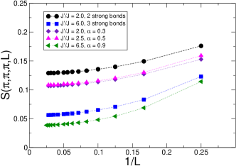
Figure 2: The $1/L$ dependence of the staggered structure factors $S(\pi,\pi,\pi,L)$ for some of the considered 3D quantum spin models on the stacked honeycomb lattice. The anisotropic factor $\alpha$ and $J^{\prime}/J$ associated with each of the presented data sets are specified in the legend. The dashed lines are added to guide the eye.

III The numerical results

To investigate the $\alpha$ dependence of the scaling relations between $T_{N}$ and $M_{s}$, particularly to understand how these universal curves shown in Refs. Tan181 get modified, we have carried out a large-scale QMC simulation using the stochastic series expansion (SSE) algorithm with very efficient operator-loop update San99 . To begin with, in the following we will firstly present our determination of $M_{s}$.

III.1 The determination of $M_{s}$

For each considered value of $J^{\prime}/J$, the associated $M_{s}$ can be derived from $S(\pi,\pi,\pi,L)$ obtained at zero temperature by $\sqrt{S(\pi,\pi,\pi,L\rightarrow\infty)}$. Here the zero temperature results of $S(\pi,\pi,\pi,L)$ are reached through simulations using $\beta=2L$. We would like to point out that for small to intermediate lattices, larger $\beta$ than $\beta=2L$ are employed. For several studied models and some selected $J^{\prime}/J$, we have additionally performed a few simulations using $\beta>2L$ (including those done with $\beta=4L$). The results obtained from these trial calculations agree very well with those explicitly presented in this investigation. Therefore, the determined $M_{s}$ shown here should be the ones corresponding to the ground states.

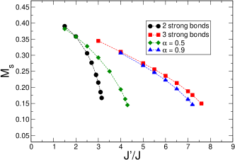
Figure 3: $M_{s}$ as functions of the considered $J^{\prime}/J$ for several of the studied 3D quantum spin models on the stacked honeycomb lattice. The anisotropic factor $\alpha$ associated with each of the presented data sets are specified in the legend. The dashed lines are added to guide the eye.

For several studied models, the $1/L$-dependence of their ground states $S(\pi,\pi,\pi,L)$ for some considered $J^{\prime}/J$ are depicted in figs. 2. Following Refs. Car96 the numerical values of $M_{s}$ are obtained by performing extrapolations in $1/L$ using the following three ansatzes

$$a_{0}+a_{2}/L^{2},$$ (7)

$$b_{0}+b_{2}/L^{2}+b_{3}/L^{3},$$ (8)

$$c_{0}+c_{2}/L^{2}+c_{3}/L^{3}+c_{4}/L^{4},$$ (9)

In particular, the corresponding results of $M_{s}$ are determined by taking the square roots of $a_{0},b_{0},c_{0}$ calculated from the fits. In some cases, formulas up to fifth order in $1/L$ are used for the fits. The calculated numerical values of $M_{s}$ for the studied models are shown in fig. 3. The data presented in that figure are obtained by averaging over all the good fits (Which are defined as those with a $\chi^{2}/{\text{DOF}}<2.0$). Furthermore, for every studied model and for each considered parameter $J^{\prime}/J$, the corresponding uncertainty shown in the figure is based on the associated errors from all the (good) fits related to it.

III.2 The determination of $T_{N}$

The Néel temperatures $T_{N}$ for various $J^{\prime}/J$ of the studied models are calculated by applying the expected finite-size scaling to the relevant observables. Specifically, $T_{N}$ are determined through bootstrap-type fits using constrained standard finite-size scaling ansatz of the form

$$(1+b_{0}L^{-\omega})(b_{1}+b_{2}tL^{1/\nu}+b_{3}(tL^{1/\nu})^{2}+...).$$ (10)

Here $b_{i}$ for $i=0,1,2,...$ are some constants and $t=\frac{T-T_{N}}{T_{N}}$. Moreover, this ansatz with up to second, third, fourth order and (or) fifth order in $tL^{1/\nu}$ are carried out to fit the data of $Q_{1}$, $Q_{2}$ and $\rho_{s}L$. The $Q_{1}$ ($Q_{2})$ data of one of the investigated models are shown in the top (bottom) panel of fig. 4.

For the considered models, the detailed steps of estimating the corresponding $T_{N}$ including their associated uncertainties are the same as those demonstrated in Ref. Tan181 . With the procedures describing in Ref. Tan181 , the $T_{N}$ obtained from the three used observables for several of the studied models are shown in figs. 5. It should be pointed out that for some cases, while the $T_{N}$ determined from considering the observable $\rho_{s}L$ are slightly different from those related to $Q_{1}$ and $Q_{2}$, the variations are merely at few per mille level. Therefore, one expects that such small discrepancies have no influence on the conclusions obtained here.

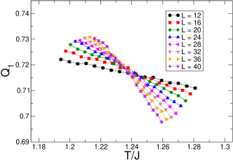
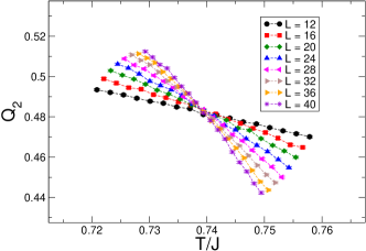
Figure 4: $Q_{1}$ (top panel, three strong bonds, $J^{\prime}/J=6.0$) and $Q_{2}$ (bottom panel, two strong bonds, $J^{\prime}/J=2.7$) as functions of $T/J$ for various $L$. The dashed lines are added to guide the eye.

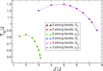
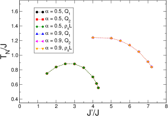
Figure 5: The $J^{\prime}/J$ dependence of $T_{N}$ obtained from $Q_{1}$, $Q_{2}$, and $\rho_{s}L$ for some considered 3D spin models studied here. The $\alpha$ corresponding to the data presented in the figure are shown explicitly in the legend. The dashed lines are added to guide the eye.

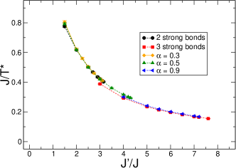
Figure 6: The inverse of $T^{\star}$ as functions of $J^{\prime}/J$ for some 3D spin models studied here. The $\alpha$ corresponding to the data presented in the figure are shown explicitly in the legend. The dashed lines are added to guide the eye.

III.3 The determination of $T^{\star}$

For all the investigated models, the temperatures at which $\chi_{u}$ reach their maximum value (These temperatures are denoted by $T^{\star}$) are determined on lattices with $L=16$. The estimations of the inverse of $T^{\star}$ as functions of $J^{\prime}/J$ for several considered systems are shown in fig. 6.

For some models, simulations with $L=32$ are conducted in order to understand the effects of finite-size on the determination of $T^{\star}$. For these additional calculations we find that the results obtained on $L=16$ lattices are already the bulk ones. Based on these studies on $L=32$ lattices as well as those presented in Refs. Tan181 , it is anticipated the conclusions obtained in the following (sub)section by employing these estimated $T^{\star}$ (on $L=16$ lattices) should be reliable.

III.4 The scaling relations between $T_{N}/\overline{J}$, $T_{N}/T^{\star}$, and $M_{s}$

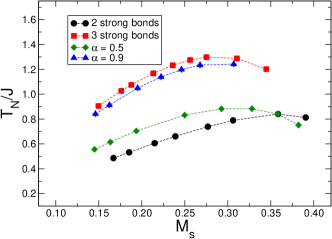
Figure 7: $T_{N}/J$ as functions of $M_{s}$ for several considered 3D dimerized models on the stacked honeycomb lattice. Each $T_{N}$ shown in the figure is obtained from $Q_{1}$. The dashed lines are added to guide the eyes.

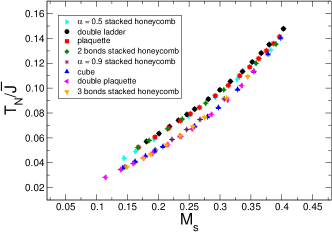
Figure 8: $T_{N}/\overline{J}$ as functions of $M_{s}$ for most of the considered models in this study. Each used $T_{N}$ in the figure is obtained from $Q_{1}$. For comparison purpose, some data presented in Ref. Tan181 are shown in the figure as well.

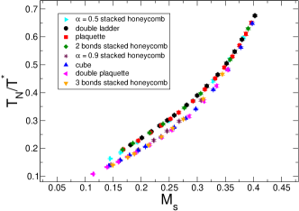
Figure 9: $T_{N}/T^{\star}$ as functions of $M_{s}$ for most of the considered models in this study. Each used $T_{N}$ in the figure is obtained from $Q_{1}$. For comparison purpose, some data presented in Ref. Tan181 are shown in the figure as well.

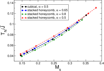
Figure 10: (Top panel) Universal curves associated with $T_{N}/\overline{J}$ and $M_{s}$ for models on the cubic ($\alpha=0.5$) and the stacked honeycomb ($\alpha=0.5,0.65,0.8$) lattices. (Bottom panel) Universal curves associated with $T_{N}/T^{*}$ and $M_{s}$ for models on the cubic ($\alpha=0.5$) and the stacked honeycomb ($\alpha=0.5,0.65,0.8$) lattices. The dashed lines are added to guide the eye. For better visualization, in the bottom panel the dashed line associated with $\alpha=0.65$ (stacked honeycomb) is not shown explicitly.

Using the $M_{s}$ and $T_{N}$ determined in the previous subsections, we find that no clear connections between the curves of $T_{N}/J$ against $M_{s}$ among these studied spin-1/2 models on the stacked honeycomb lattice, see fig. 7 for the outcomes of several considered systems. Interestingly, if $T_{N}/\overline{J}$ are plotted as functions of $M_{s}$, universal scaling relations emerges, as can been seen in fig. 8. Remarkably, while for systems of $\alpha=0.3$ (not shown in fig. 8) and $0.5$, as well as model with two strong bonds attaching to each of its spin, the resulting data of $T_{N}/\overline{J}$ as functions of $M_{s}$ do form a universal curve, this universal curve falls on top of the one corresponding to the models investigated in Ref. Tan181 which have two strong bonds connected to each of their spin. Similar situation occurs for models with $\alpha=0.9$ and that having three strong bonds emerging from each spin, namely all of their associated data form a single curve. In particular, this universal curve matches the one related to the cubic and double plaquette models investigated in Ref. Tan181 . Finally, we would like to emphasize the fact that the data obtained for other values of $\alpha$ here indicate as the magnitude of $\alpha$ increases from 0.5 to 0.9, the resulting curves begin to deviate from the curve associated with two strong bonds and eventually collapse with the curve corresponding to three strong bonds.

By considering $T_{N}/T^{\star}$ as functions of $M_{s}$ for all the models studied here as well as those investigated in Ref. Tan181 , the same scenario as that of $T_{N}/\overline{J}$ versus $M_{s}$ also appears, see fig. 9.

It is remarkably that the classification schemes which are firstly pointed out in Ref. Tan181 and are valid for cubic type lattices are now extended to include 3D quantum spin models on the stacked honeycomb lattice. While this is the case, effects due to microscopic details, specially those of the quantum fluctuations, do have minor impact on the categorization of the universal curves. Indeed, as can be seen from figs. 8 and 9, when the magnitude of $M_{s}$ increases, the curve related to the models of three strong bonds and $\alpha=0.9$ studied here begins to move toward the curve associated with two strong bonds at a value $M_{s}$ slightly smaller than that of the curve resulting from the models considered in Ref. Tan181 . Since the stacked honeycomb lattice has five coordinate number which is fewer than those of the cubic and the double cubic lattices, the resulting quantum fluctuation is more profound and have greater influence on properties of the systems on the stacked honeycomb lattice. Nevertheless, it is beyond doubt that the classification schemes claimed in Ref. Tan181 are valid not only on cubic-type lattices, but also for models on the stacked honeycomb lattice. In particular, the universal curves associated with the stacked honeycomb lattice match those related to the cubic-type lattices.

We would like to point out that while intuitively one expects the curve related to a particular value of $\alpha$ will start to move away from the one of two strong bonds, it in intriguing that this particular $\alpha$ is larger than (equal to) $0.5$ for the models on the stacked honeycomb lattice studied here.

Apart from quantum spin models on the stacked honeycomb lattice, we have additionally simulated the cubic model studied in Ref. Tan181 . In particular, an anisotropic bond similar to the $\alpha$-bond considered here is introduced in our investigation so that models with three types of bonds can be obtained, see the left bottom panel of fig. 1. This generalized model will be called anisotropic cubic model. Remarkably, the $T_{N}/\overline{J}$ and $T_{N}/T^{*}$ versus $M_{s}$ data for $\alpha=0.5$ on the anisotropic cubic model fall on the same curve as that of the model on the stacked honeycomb lattice with $\alpha=0.65$, see fig. 10. The associated data for $\alpha=0.8$ and $\alpha=0.5$ of the models on the stacked honeycomb lattice are also shown in fig. 10. With these two additional sets of data, one can sees clearly the good data collapse quality from both the systems on the anisotropic cubic lattice with $\alpha=0.5$ and on the stacked honeycomb lattice with $\alpha=0.65$. The outcomes demonstrated in both top and bottom panels of fig. 10 suggest convincingly that there is yet a to be understood categorization rule for the anisotropic models with $0<\alpha<1$.

Besides the results presented above, another compelling outcome from our investigation is that for both lattice geometries, data collapse of $T_{N}/\overline{J}$ ($T_{N}/T^{\star}$) versus $M_{s}$ with $\alpha=0.5$ within each category of lattice geometries (and $\alpha=0.8$ on the stacked honeycomb lattice) lead to a smooth curve, see both panels of fig. 11. Specifically, the curves of related data of both models on the top (bottom) panel of fig. 1 with $\alpha=0.5$ ($\alpha=0.5$), which are different models on the stacked honeycomb (cubic) lattice, fall on top of each other. The situation also occurs for models of $\alpha=0.8$ associated with the stacked honeycomb lattice, but its universal curve differs from the one of $\alpha=0.5$. Based on these outcomes, it is highly probable that such a scenario occurs for other values of $\alpha$. This result strongly suggests that for each value of spatial anisotropy, the universal characteristics between $T_{N}$ and $M_{s}$, which were found in Refs. Jin12 ; Tan181 can be classified by the coordinate number of the underlying lattice geometries. This observation for 3D anisotropic quantum spin systems is new, and was not established before in the literature. We would like to emphasize the fact that in fig. 11 the quality of data collapse for the two different models on the stacked honeycomb lattice is much better than those of the systems on the cubic lattice. It might be interesting to understand this result from a theoretical point of view.

Finally, it should be pointed out that although $\overline{J}$ and $T^{\star}$ are two completely different quantities, it is remarkable that based on the results presented in Refs. Jin12 ; Tan181 and here, the categorization schemes for $T_{N}/\overline{J}$ versus $M_{s}$ and $T_{N}/T^{\star}$ versus $M_{s}$ are totally identical to each other. This implies there may be an even more fundamental classification principle than those already explored.

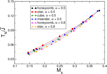
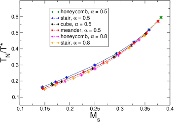
Figure 11: (Top panel) Universal curves associated with $T_{N}/\overline{J}$ and $M_{s}$ for models on both the cubic ($\alpha=0.5$) and the stacked honeycomb ($\alpha=0.5,0.8$) lattices. (Bottom panel) Universal curves associated with $T_{N}/T^{*}$ and $M_{s}$ for models on both the cubic ($\alpha=0.5$) and the stacked honeycomb ($\alpha=0.5,0.8$) lattices. The dashed lines are added to guide the eyes.

IV Discussions and Conclusions

Using the first principles quantum Monte Carlo simulations, we have investigated in detail the universal scaling relations between $T_{N}$ and $M_{s}$, namely $T_{N}/\overline{J}$ versus $M_{s}$ and $T_{N}/T^{\star}$ versus $M_{s}$ for 3D quantum antiferromagnets on both the stacked honeycomb and the cubic lattices.

By studying the 3D spin-1/2 dimerized Heisenberg models with two types of antiferromagnetic coupling strength, in Ref. Tan181 it was established that these universal relations can be classification by the number of $J^{\prime}$-bonds touching each spin of the considered models. Here we extend these categorization schemes by investigating systems with three kinds of bonds and on lattices of different geometries.

According to the outcomes obtained here, while the classification rules for anisotropic cases are more complicated than the ones established in Ref. Tan181 , without doubt a generalized categorization principle does exist for these models with $0<\alpha<1$. Particularly, we conjecture that with the presence of three types of bonds and for a given $\alpha$, the categorization rule is in accordance with the coordinate number of the underlying lattice geometry. More surprisingly, although $T^{\star}$ and $\overline{J}$ are two completely different physical quantities, the classification schemes for these two relations are identical.

To understand the theories relevant to the results obtained here, particularly to uncover the corresponding mechanism behind the identical classification schemes for two different universal relations observed in this study, will definitely be interesting and compelling to pursue in the future.

V Acknowledgments

This study is partially supported by MOST of Taiwan.

References

- (1) Nigel Goldenfeld, Lectures On Phase Transitions And The Renormalization Group (Frontiers in Physics) (Addison-Wesley, 1992).
- (2) Lincoln D. Carr, Understanding Quantum Phase Transitions (Condensed Matter Physics) (CRC Press, 2010).
- (3) S. Sachdev, Quantum Phase Transitions (Cambridge University Press, Cambridge, 2nd edition, 2011).
- (4) M. Campostrini, M. Hasenbusch, A. Pelissetto, P. Rossi, and E. Vicari, Phys. Rev. B 65, 144520 (2002).
- (5) Andrea Pelissetto and Ettore Vicari, Physics Reports 368 (2002) 549-727.
- (6) A. V. Chubukov and S. Sachdev, Phys. Rev. Lett. 71, 169 (1993).
- (7) A. V. Chubukov and S. Sachdev, Phys. Rev. Lett. 71, 2680 (1993).
- (8) A. V. Chubukov, S. Sachdev, and J. Ye, Phys. Rev. B 49, 11919 (1994).
- (9) A. W. Sandvik, A. V. Chubukov, and S. Sachdev, Phys. Rev. B 51, 16483 (1995)
- (10) M. Troyer, H. Kantani, and K. Ueda, Phys. Rev. Lett. 76, 3822 (1996).
- (11) Matthias Troyer, Masatoshi Imada, and Kazuo Ueda, J. Phys. Soc. Jpn. 66, 2957 (1997).
- (12) Jae-Kwon Kim and Matthias Troyer, Phys. Rev. Lett. 80, 2705 (1998).
- (13) Y. J. Kim and R. J. Birgeneau, Phys. Rev. B 62, 6378 (2000).
- (14) A. Sen, H. Suwa, and A. W. Sandvik, Phys. Rev. B 92, 195145 (2015).
- (15) D.-R. Tan and F.-J. Jiang, Phys. Rev. B 98, 245111 (2018).
- (16) Ch. Rüegg, N.Cavadini, A. Furrer, H.-U. Güdel, K. Krämer, H. Mutka, A. Wildes, K. Habicht, and P. Vorderwisch, Nature (London) 423, 62, (2003).
- (17) Ch. Rüegg et al., Phys. Rev. Lett. 100, 205701 (2008).
- (18) P. Merchant, B. Normand, K. W. Krämer, M. Boehm, D. F. McMorrow, and Ch. Rüegg, Nature physics 10, 373-379 (2014).
- (19) Y. Kulik, and O. P. Sushkov, Phys. Rev. B 84, 134418 (2011).
- (20) J. Oitmaa, Y. Kulik, and O. P. Sushkov, Phys. Rev. B 85, 144431 (2012).
- (21) S. Jin and A. W. Sandvik, Phys. Rev. B 85, 020409(R) (2012).
- (22) M.-T. Kao and F.-J. Jiang, Eur. Phy. J. B, (2013) 86: 419.
- (23) Yan Qi Qin, Bruce Normand, Anders W. Sandvik, and Zi Yang Meng, Phys. Rev. B 92, 214401 (2015).
- (24) Harley Scammell and Oleg Sushkov, Phys. Rev. B 92, 220401 (2015).
- (25) Deng-Ruei Tan and Fu-Jiun Jiang, Eur. Phys. J. B, (2015) 88 : 289.
- (26) Harley Scammell and Oleg Sushkov, Phys. Rev. B 95, 024420 (2017).
- (27) Harley Scammell and Oleg Sushkov, Phys. Rev. B 95, 094410 (2017).
- (28) D.-R. Tan and F.-J. Jiang, Phys. Rev. B 95, 054435 (2017).
- (29) H. D. Scammell, Y. Kharkov, Yan Qi Qin, Zi Yang Meng, B. Normand, and O. P. Sushkov, Phys. Rev. B 96, 174414 (2017).
- (30) D.-R. Tan, C.-D. Li, and F.-J. Jiang, Phys. Rev. B 97, 094405 (2018).
- (31) Most of the simulations are done with . Here we use to stand for unless specified.
- (32) A. W. Sandvik, Phys. Rev. B 56, 18 (1997).
- (33) A. W. Sandvik, Phys. Rev. B 66, R14157 (1999).
- (34) J. Cardy, Scaling and Renormalization in Statistical Physics (Cambridge University Press, Cambridge, 1996).