Link homology theories and ribbon concordances

Abstract.

It was recently proved by several authors that ribbon concordances induce injective maps in knot Floer homology, Khovanov homology, and the Heegaard Floer homology of the branched double cover. We give a simple proof of a similar statement in a more general setting, which includes knot Floer homology, Khovanov-Rozansky homologies, and all conic strong Khovanov-Floer theories. This gives a philosophical answer to the question of which aspects of a link TQFT make it injective under ribbon concordances.

1. Introduction

Given two knots $K_{1}$ and $K_{2}$, smoothly embedded in $S^{3}$, a (smooth) cobordism from $K_{1}$ to $K_{2}$ is a smoothly embedded surface $S$ in $S^{3}\times I$ such that $\partial C=(K_{1}\times\{0\})\sqcup(K_{2}\times\{1\})$. A connected cobordism is called a concordance its genus is zero. By endowing $S$ with a Morse function, it is easy to see that every knot (or, in general, link) cobordism consists of births, saddles, and deaths; when $S$ is a concordance and there are no deaths needed to construct $S$, we say that $S$ is a ribbon concordance.

Unlike the knot concordance relation, which is symmetric, having a ribbon concordance from a knot to another is not a symmetric relation. It is conjectured by Gordon[Gor81] that existence of a ribbon concordance induces a partial order on each knot concordance class. There are several results in that direction, starting with Gordon’s result[Gor81], that if $C$ is a ribbon concordance from $K_{1}$ to $K_{2}$, then the map $\pi_{1}(S^{3}\backslash K_{1})\rightarrow\pi_{1}((S^{3}\times I)\backslash C)$ is injective and $\pi_{1}(S^{3}\backslash K_{2})\rightarrow\pi_{1}((S^{3}\times I)\backslash C)$ is surjective.

Recently, it was proved by Zemke[Zem19a] that, after endowing $C$ with a suitable decoration, the cobordism map

$$\hat{F}_{C}:\widehat{HFK}(K_{1})\rightarrow\widehat{HFK}(K_{2})$$

is injective, so that if there exists a ribbon concordance from $K_{1}$ to $K_{2}$ and also from $K_{2}$ to $K_{1}$, then $\widehat{HFK}(K_{1})\simeq\widehat{HFK}(K_{2})$ as bigraded vector spaces. This result was then extended to other link homology theories. For example, Levine and Zemke[LZ19] proved that the map

$$\mathbf{Kh}(C):\mathbf{Kh}(K_{1})\rightarrow\mathbf{Kh}(K_{2})$$

is injective. Later, Lidman, Vela-Vick, and Wong [LVVW19] proved that the map

$$\hat{F}_{\Sigma(C)}:\widehat{HF}(\Sigma(K_{1}))\rightarrow\widehat{HF}(\Sigma(K_{2}))$$

is also injective, where $\Sigma(K_{i})$ is the branched double cover of $S^{3}$ along $K_{i}$ and $\Sigma(C)$ is the branched double cover of $S^{3}\times I$ along $C$. Note that $\Sigma(C)$ is a 4-dimensional smooth cobordism from the 3-manifold $\Sigma(K_{1})$ to $\Sigma(K_{2})$.

However, the proofs of the above results rely on some special properties that the link homology theories $\widehat{HFL}$, $\mathbf{Kh}$, and $\widehat{HF}\circ\Sigma$ have. The proof of injectivity for $\widehat{HFK}$ depends on its generalization to a TQFT of null-homologous links in 3-manifolds, and the proof for $\mathbf{Kh}$ uses the fact that it satisfies the neck-cutting relation in the dotted cobordism category. Furthermore, the proof for $\widehat{HF}\circ\Sigma$ uses graph cobordisms, defined and studied originally by Zemke[Zem15].

In this paper, we give a simple proof of the injectivity of maps induced by ribbon concordance in a much more general setting. The link homology theories that we can use are multiplicative link TQFTs which are either associative or Khovanov-like, whose definitions will be given in the next section. In particular, our main theorem is the following.

Theorem 1.

Let $C$ be a ribbon concordance and $F$ be a multiplicative TQFT of oriented links in $S^{3}$, which is either associative or Khovanov-like. Then $F(C)$ is injective, and $F(\bar{C})$ is its left inverse.

The notion of associativity and Khovanov-like-ness, together with multiplicativity, is so general that they include all conic strong Khovanov-Floer theories, defined in [Sal17], which is based on the definition of Khovanov-Floer theories in [BHL19], and all Khovanov-Rozansky homologies, which were first defined in [KR04]. This gives us the following corollaries.

Corollary 2.

Let $C$ be a ribbon concordance and $F$ be either a conic strong Khovanov-Floer theory or Khovanov-Rozansky $\mathfrak{gl}(n)$-homology for some $n\geq 2$. Then $F(C)$ is injective.

Corollary 3.

Let $K_{1}$ and $K_{2}$ be knots, such that there exists a ribbon concordance $C$ from $K_{1}$ to $K_{2}$, and $C^{\prime}$ from $K_{2}$ to $K_{1}$. Then for any link TQFT $F$ which is either a conic strong Khovanov-Floer theory or a Khovanov-Rozansky homology, we have $F(K_{1})\cong F(K_{2})$.

Furthermore, we will observe that if $F$ is actually a $\mathbb{Z}$-graded theory, and satisfies some nice properties, then our proof of injectivity simplifies even more.

As a topological application of our arguments, we will give a very simple alternative proof of Zemke’s result on knot Floer homology. Then we will also give another proof of Lidman-Vela-Vick-Wong’s result on $\widehat{HF}\circ\Sigma$ and prove the following theorem, regarding the deck transformation action, denoted as $\tau$, and the involution introduced in [HM⁺17], denoted as $\iota$, on the hat-flavor Heegaard Floer homology of branched double covers.

Theorem 4.

Suppose that a knot $K_{0}$ is ribbon concordant to $K_{1}$. Then the following statements hold.

• If $K_{1}$ is an odd torus knot, then the $\tau$-action on $\widehat{HF}(\Sigma(K_{0}))$ are trivial.

• If $K_{1}$ is a Montesinos knot, then the $\tau$-action and the $\iota$-action on $\widehat{HF}(\Sigma(K_{0}))$ coincide, and there exists a $\tau$-invariant basis of $\widehat{HF}(\Sigma(K_{0}))$ with only one fixed basis element.

Acknowledgement

The author would like to specially thank Marco Marengon for suggesting an idea for the proof of the nicely graded case. The author is also grateful to Abhishek Mallick for helpful discussions, and Monica Jinwoo Kang, Andras Juhasz and Robert Lipshitz for numerous helpful comments on this paper. Finally, the author would also like to thank University of Oregon and UCLA for their hospitality.

2. Multiplicative link TQFTs and conic strong Khovanov-Floer theories

2.1. Multiplicativity of a TQFT of links in $S^{3}$

Recall that a (vector space valued) TQFT $F$ of (oriented) links in $S^{3}$ is a functor

$$F:\mathbf{Link}_{S^{3}}^{+}\rightarrow\mathbf{Vect}_{\mathbb{F}}.$$

Here, $\mathbf{Link}_{S^{3}}^{+}$ is the category whose objects are oriented links in $S^{3}$ and morphisms are oriented link cobordisms, and $\mathbf{Vect}_{\mathbb{F}}$ is the category of vector spaces over a fixed coefficient field $\mathbb{F}$.

Suppose that a link $L$ can be written as a disjoint union $L=L_{1}\sqcup L_{2}$, i.e. there exists a genus zero Heegaard splitting $S^{3}=D_{1}\cup_{S^{2}}D_{2}$ such that $L\cap S^{2}=\emptyset$, $L\cap D_{1}=L_{1}$, and $L\cap D_{2}=L_{2}$. Then we usually expect $F(L)$ to split along the disjoint union as follows:

$$F(L)\simeq F(L_{1})\otimes_{\mathbb{F}}F(L_{2}).$$

But the multiplicativity that we want $F$ to satisfy is stronger than having such an isomorphism. Suppose that we are given link cobordisms

$$S_{1} :L_{1}\rightarrow L_{1}^{\prime},$$

$$S_{2} :L_{2}\rightarrow L_{2}^{\prime},$$

and consider the links $L=L_{1}\sqcup L_{2}$ and $L^{\prime}=L_{1}^{\prime}\sqcup L_{2}^{\prime}$. When there exist disjoint open balls $V_{1},V_{2}\subset S^{3}$, satisfying $L_{1}\subset V_{1}$ and $L_{2}\subset V_{2}$, such that $S_{1}\subset V_{1}\times I$ and $S_{2}\subset V_{2}\times I$, we can form the disjoint union cobordism $S=S_{1}\sqcup S_{2}$. The cobordism $S$ is then a link cobordism from $L$ to $L^{\prime}$.

Now we have three linear maps:

$$F(S_{1}) :F(L_{1})\rightarrow F(L_{1}^{\prime}),$$

$$F(S_{2}) :F(L_{2})\rightarrow F(L_{2}^{\prime}),$$

$$F(S) :F(L)\rightarrow F(L^{\prime}).$$

Using these maps, we define the multiplicativity of $F$ as follows.

Definition 5.

A TQFT of (oriented) links in $S^{3}$ is multiplicative if we have identifications

$$F(L) \simeq F(L_{1})\otimes F(L_{2}),$$

$$F(L^{\prime}) \simeq F(L_{1}^{\prime})\otimes F(L_{2}^{\prime}),$$

such that $F(S)=F(S_{1})\otimes F(S_{2})$ is satisfied.

Unfortunately, multiplicativity is not enough to prove that all ribbon concordance induce injective maps, so we need to introduce some additional conditions on multiplicative link TQFTs.

Definition 6.

A multiplicative TQFT $F$ of oriented links in $S^{3}$ is associative if for any link $L=L_{1}\sqcup L_{2}$ such that $L_{1},L_{2}$ are contained in disjoint open balls $V_{1},V_{2}$ respectively, we have an associated isomorphism

$$F(L)\xrightarrow{\cong}F(L_{1})\otimes F(L_{2})$$

which depends only on the choice of open balls $V_{1}$ and $V_{2}$, and if we are given a link $L=L_{1}\sqcup L_{2}\sqcup L_{3}$, the following diagram commutes.

As we will see in the next section, associativity is enough to prove that ribbon concordance maps are injective. However, even when we are given with a link TQFT which is multiplicative but not associative, we are still able to find another condition which is sufficient for our goal.

Recall that, if $F$ is a TQFT of (oriented) links in $S^{3}$, then the $\mathbb{F}$-vector space $F(\text{unknot})$ comes with the following operations:

$$\text{birth map }b: \mathbb{F}\rightarrow F(\text{unknot}),$$

$$\text{death }\epsilon: F(\text{unknot})\rightarrow\mathbb{F}.$$

Also, we call the element $b(1)\in F(\text{unknot})$ as the unit and denote it as $u$. Note that, if $F$ is the Khovanov homology functor $\mathbf{Kh}$, then $\epsilon(u)=0$ and $u$ spans the kernel of $\epsilon$.

Definition 7.

A multiplicative TQFT $F$ of oriented links in $S^{3}$ is Khovanov-like if the unit $u\in F(\text{unknot})$ spans the kernel of the counit $\epsilon$.

2.2. Khovanov-Floer theories

The notion of Khovanov-Floer theory first appeared in [BHL19]. In that paper, Baldwin, Hedden, and Lobb gave its definition as follows.

Definition 8.

Let $V$ be a graded vector space. a $V$-complex is a pair $(C,q)$ where $C$ is a filtered chain complex and $q:V\rightarrow E_{2}(C)$ is an isomorphism. A map of $V$-complexes is a filtered chain map. When a map $f$ of $V$-complexes induces the identity map between the $E_{2}$ pages, we say that $f$ is a quasi-isomorphism.

Definition 9.

A Khovanov-Floer theory $\mathcal{A}$ is a rule which assigns to every link diagram $D$ a quasi-isomorphism class $\mathcal{A}(D)$ of $\mathbf{Kh}(D)$-complexes which satisfies the following conditions.

• If $D^{\prime}$ is planar isotopic to $D$, then there is a morphism $\mathcal{A}(D)\rightarrow\mathcal{A}(D^{\prime})$ which induces the isotopy map $\mathbf{Kh}(D)\xrightarrow{\sim}\mathbf{Kh}(D^{\prime})$ on the $E_{2}$ page.

• If $D^{\prime}$ is obtained from $D$ by a diagrammatic 1-handle attachment, then there is a morphism $\mathcal{A}(D)\rightarrow\mathcal{A}(D^{\prime})$ which induces the cobordism map $\mathbf{Kh}(D)\rightarrow\mathbf{Kh}(D^{\prime})$ on the $E_{2}$ page.

• For any diagrams $D,D^{\prime}$, we have a morphism $\mathcal{A}(D\sqcup D^{\prime})\rightarrow\mathcal{A}(D)\otimes\mathcal{A}(D^{\prime})$ which induces the standard isomorphism $\mathbf{Kh}(D\sqcup D^{\prime})\xrightarrow{\sim}\mathbf{Kh}(D)\otimes\mathbf{Kh}(D^{\prime})$ on the $E_{2}$ page.

• If $D$ is a diagram of an unlink, then the spectral sequence $E_{2}(\mathcal{A}(D))\Rightarrow E_{\infty}(\mathcal{A}(D))$ degenerates on the $E_{2}$ page.

Later, Saltz gave a definition of strong Khovanov-Floer theories in the following way.

Definition 10.

A strong Khovanov-Floer theory $\mathcal{K}$ is a rule which assigns a link diagram $D$ and a collection of auxiliary data $A$ a filtered chain complex $\mathcal{K}(D,A)$ satisfying the following conditions.

• For any two collections $A_{\alpha},A_{\beta}$ of auxiliary data, there is a homotopy equivalence $a_{\alpha}^{\beta}:\mathcal{K}(D,A_{\alpha})\rightarrow\mathcal{K}(D,A_{\beta})$. We write $\mathcal{K}(D)$ for the canonical representative of the transitive system $\{\mathcal{K}(D,A_{\alpha}),a_{\alpha}^{\beta}\}$, i.e. the limit of the diagram $\{\mathcal{K}(D,A_{\alpha}),a_{\alpha}^{\beta}\}$ in the homotopy category of chain complexes.

• If $D$ is a crossingless diagram of the unknot, then $H_{\ast}(\mathcal{K}(D))\simeq\mathbf{Kh}(D)$.

• For diagrams $D,D^{\prime}$, we have $\mathcal{K}(D\sqcup D^{\prime})\simeq\mathcal{K}(D)\otimes K(D^{\prime})$.

Furthermore, a strong Khovanov-Floer theory also assigns maps to diagrammatic cobordisms with auxiliary data. Those maps should satisfy the following conditions.

• If $D^{\prime}$ is obtained from $D$ by a diagrammatic handle attachment, then there is a function

  $$\phi:\{\text{auxiliary data for }D\}\rightarrow\{\text{auxiliary data for }D^{\prime}\}$$

  and a map

  $$\mathfrak{h}_{A_{\alpha},\phi(A_{\alpha}),B}:\mathcal{K}(D,A_{\alpha})\rightarrow\mathcal{K}(D^{\prime},\phi(A_{\alpha})$$

  where $B$ is some additional auxiliary data. In addition, if the domain of $\phi$ is empty, then its codomain is also empty. This gives a well-defined map

  $$\mathfrak{h}_{B}:\mathcal{K}(D)\rightarrow\mathcal{K}(D^{\prime})$$

  for a fixed $B$. Furthermore, for any two sets $B,B^{\prime}$ of additional auxiliary data, we have $\mathfrak{h}_{B}\simeq\mathfrak{h}_{B^{\prime}}$.

• If $D$ is a crossingless diagram of the unknot, then $\mathcal{K}(D)$ is isomorphic to $\mathbf{Kh}(D)$ as Frobenius algebras.

• If $D^{\prime}$ is obtained from $D$ by a planar isotopy, then $\mathcal{K}(D)\simeq\mathcal{K}(D^{\prime})$.

• Let $D=D_{0}\sqcup D_{1}$, $D^{\prime}=D_{0}^{\prime}\sqcup D_{1}^{\prime}$, and suppose that $\Sigma_{0},\Sigma_{1}$ are diagrammatic cobordisms from $D_{0}$ to $D_{0}^{\prime}$ and $D_{1}$ to $D_{1}^{\prime}$, respectively. Take the disjoint union $\Sigma=\Sigma_{0}\sqcup\Sigma_{1}$. Then we have

  $$\mathcal{K}(\Sigma)=\mathcal{K}(\Sigma_{0})\otimes\mathcal{K}(\Sigma_{1}).$$

• The handle attachment maps are invariant under swapping the order of handle attachments with disjoint supports, and satisfies movie move 15, as shown in Figure 2 of [Sal17].

Unfortunately, for a strong Khovanov-Floer theory to induce a TQFT of links in $S^{3}$, we need one more condition.

Definition 11.

A strong Khovanov-Floer theory $\mathcal{K}$ is conic if for any link diagram $D$ and any crossing $c$ of $D$, we have

$$\mathcal{K}(D)\simeq\text{Cone}(\mathcal{K}(D_{0})\xrightarrow{\mathfrak{h}_{\gamma_{c}}}\mathcal{K}(D_{1})),$$

where $D_{0}$ and $D_{1}$ are the 0-resolution and the 1-resolution of $D$ at $c$ and $\mathfrak{h}_{\gamma_{c}}$ is the diagrammatic handle attachment map at $c$.

The notion of conic strong Khovanov-Floer theories is very general. The following list of link homology theories are examples of conic strong Khovanov-Floer theories. (Actually, all strong Khovanov-Floer theories known up to now are conic!)

• Khovanov homology of $L$[Kho99];

• Heegaard Floer homology of $\Sigma(\text{unknot}\sqcup L)$[OS05];

• Unreduced singular instanton homology of $L$[KM11];

• Bar-Natan homology of $L$[Ras10];

• Szabo homology of $L$[Sza10].

When $\mathcal{K}$ is a conic strong Khovanov-Floer theory, its homology $K=H_{\ast}(\mathcal{K})$ is functorial under link cobordisms in $S^{3}\times I$, and thus a Khovanov-like multiplivative TQFT, by Theorem 5.9 of [Sal17]. Hence we see that our conditions on link TQFTs are general enough to cover all strong Khovanov-Floer theories. Actually, even more is true: all strong Khovanov-Floer theories known up to now are associative. But it is not clear whether the same should also be true for all strong theories.

In this paper, we will confuse Khovanov-Floer theories with their homology, so that when we say that $F$ is a conic strong Khovanov-Floer theory, we will actually mean that $F$ is the multiplicative link TQFT which arises as the homology of a conic strong Khovanov-Floer theory.

3. Proof of Theorem 1

3.1. An alternative decomposition of a saddle followed by the dual saddle

Let a link $L$ and a framed simple arc $a$ inside $S^{3}$, where the interior of $a$ is disjoint from $L$ and $\partial a\subset L$, are given. Then we can perform a saddle move along $a$to $L$. In terms of cobordisms in $S^{3}\times I$, this corresponds to attaching a 1-handle; denote the saddle cobordism as $S_{a}$. Then its upside-down cobordism $\overline{S_{a}}$ can be considered as performing a “dual saddle” move, which is a saddle move along a dual arc $a^{\ast}$, as drawn in the right of Figure 3.1.

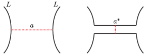
Figure 3.1. The framed arc $a$ and the dual arc $a^{\ast}$.

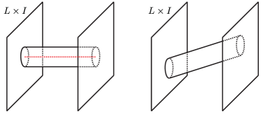
Figure 3.2. The surface $\overline{S_{a}}\circ S_{a}$ and its slight perturbation along the cylinder part

The composition $\overline{S_{a}}\circ S_{a}$ is then, topologically, a “cylinder” attached to $L\times I$, as shown in the left side of Figure 3.2. Now consider perturbing the cylinder part of our cobordism $\overline{S_{a}}\circ S_{a}$, so that one end of the cylinder part lies “below” the other end. That gives another decomposition of $\overline{S}_{a}\circ S_{a}$, as follows:

• Saddle move from $L$ to $L\sqcup U$, where the unknot component $U$ is created at one end of the arc $a$.

• Isotopy of the component $U$, along the arc $a$. This moves $U$ to the other end of $a$.

• Saddle move from $L\sqcup U$ to $L$.

Note that, in terms of movies of links, one can write the above decomposition as drawn in the right of Figure 3.3.

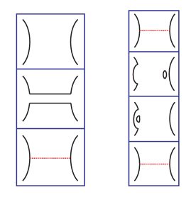
Figure 3.3. The movie on the left represents the saddle along $a$ followed by the saddle along $a^{\ast}$. The movie on the right represents our new decomposition of $\overline{S_{a}}\circ S_{a}$. Here, $U$ is the unknot component appearing in the middle of the right movie that is isotoped along $a$.

3.2. Weak neck-passing relation

Consider the 2-component unlink $U_{2}$. Then we can consider an isotopy $\phi=\{\phi_{t}\}$ from $U_{2}=A\sqcup B$ to itself, defined by moving one of its components, say $A$, around the other component $B$, as shown in Figure 3.4. This gives a link cobordism $S_{\phi}$ from $U_{2}$ to itself, as follows:

$$S_{\phi}=\bigcup_{t\in[0,1]}\phi_{t}(U_{2})\times\{t\}\subset S^{3}\times[0,1].$$

So, given any link TQFT $F$, we have a map $F(S_{\phi})\in\text{Aut}(F(U_{2}))$. We consider the following relation for multiplicative link TQFTs:

Weak  neck-passing  relation:

Let $F(U_{2})\simeq F(A)\otimes F(B)$ be the isomorphism given by the multiplicativity of $F$. Then for any element $a\in F(U_{2})$ of the form $a=x\otimes u$, where $u$ is the unit in the Frobenius algebra $F(B)$, we have $F(S_{\phi})(a)=a$.

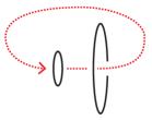
Figure 3.4. The “go-around” isotopy $\phi$ from $U_{2}$ to itself.

We now prove that any multiplicative TQFT $F$ of (oriented) links in $S^{3}$ satisfies the weak neck-passing relation. Consider the birth $B_{1}$ of the component $B$, as shown in Figure 3.5. Then $S_{\phi}\circ B_{1}$ is isotopic to $B_{2}$. But since we are working with links in $S^{3}$, not $\mathbb{R}^{3}$, we know that $B_{1}$ and $B_{2}$ are isotopic by isotoping $B_{1}$ across the point at infinity. So we have

$$F(B_{1})=F(B_{2})=(\text{birth map on }B\text{ component}).$$

Hence we get

$$F(S_{\phi})(x\otimes u)=F(S_{\phi})(F(B_{1})(x))=F(S_{\phi}\circ B_{1})(x)=F(B_{2})(x)=x\otimes u.$$

Therefore the weak neck-passing relation holds for $F$.

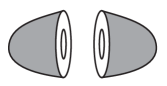
Figure 3.5. Two “birth cobordisms” $B_{1}$ and $B_{2}$ of a component in $U_{2}$.

3.3. Unknotting a ribbon concordance

Let $C$ be a ribbon concordance from a knot $K\subset S^{3}$ and $F$ be a multiplicative TQFT of (oriented) links in $S^{3}$. Then $C$ can be decomposed as $n$ births of new unknot components $U_{1},\cdots,U_{n}$ followed by saddles along framed arcs $a_{i}$ which connect $K$ with $U_{i}$. Then $\bar{C}\circ C$ is a composition of the following four types of cobordisms:

• Births of $U_{1},\cdots,U_{n}$;

• Saddles along $a_{1},\cdots,a_{n}$;

• Saddles along the dual arcs $b_{1},\cdots,b_{n}$, where $b_{i}$ is dual to $a_{i}$;

• Deaths of $U_{1},\cdots,U_{n}$.

But we can see that $\bar{C}\circ C$ also admits another decomposition into elementary cobordisms, using the observations we made in subsection 3.1. In particular, it can be realized as follows (as in Figure 3.6):

• Births of $U_{1},\cdots,U_{n}$;

• Saddles along arcs $e_{1},\cdots,e_{n}$, where the endpoints of $e_{i}$ are given by the two points in $\partial(\nu(K\cap a_{i}))\cap K$;

  • Note that this move creates a new set $U_{1}^{\prime}\cdots,U_{n}^{\prime}$ of unknot components.

• Isotopy of each $U_{i}^{\prime}$ along the framed arc $a_{i}$;

• Saddles between each pair $U_{i}$ and $U_{i}^{\prime}$, so that they merge into one unknot $U_{i}$;

• Deaths of $U_{1},\cdots,U_{n}$.

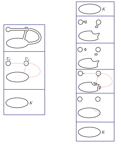
Figure 3.6. The movie on the left represents $C$, and the movie on the right represents $\bar{C}\circ C$. Here, the dotted red lines denote the framed arcs $a_{i}$, and the dotted red arrows denote the path along which we isotope the newly created unknot components $U_{i}^{\prime}$.

Choose a set of pairwise disjoint disks $\{D_{1},\cdots,D_{n}\}$, each of which is disjoint from $K$, such that $\partial D_{i}=U_{i}$ for each $i$. Then we can consider the number $n(C)$, defined as follows:

$$n(C)=\sum_{i,j}|a_{i}\cap D_{j}|,$$

assuming that all intersections between arcs $a_{i}$ and disks $D_{j}$ are transverse. From now on, we will apply an induction on $n(C)$ to prove Theorem 1; note that $n(C)$ only depends on $C$ and the choice of $U_{1},\cdots,U_{n}$ and $D_{1},\cdots,D_{n}$, and is always a nonnegative integer.

3.3.1. The base case

We first consider the base case, which is the case when $n(C)=0$. Consider the sub-cobordism $S$ of $\bar{C}\circ C$, defined as the composition of the following elementary cobordisms:

• Saddles along $e_{1},\cdots,e_{n}$, so that a new set $U_{1}^{\prime}\cdots,U_{n}^{\prime}$ of unknot components is created;

• Isotopies of each $U_{i}^{\prime}$ along the framed arc $a_{i}$.

Also, consider the cobordism $S_{0}$ from an unknot $U$ to the empty link, defined as the composition of the following elementary cobordisms:

• Birth of a new unknot component $U^{\prime}$;

• Saddle between $U$ and $U^{\prime}$, so that they merge into an unknot $U$;

• Death of $U$.

A figure depicting the cobordisms $S$ and $S_{0}$ is drawn in Figure 3.7.

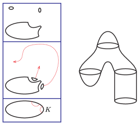
Figure 3.7. A movie for the cobordism $S$(left) and a figure representing the cobordism $S_{0}$(right). Again, the dotted red lines denote the framed arcs $a_{i}$, and the dotted red arrows denote the path along which we isotope the newly created unknot components $U_{i}^{\prime}$.

Then, by assumption, the arcs $a_{i}^{\prime}$ never pass through the disks $D_{j}$, so we have an isotopy

$$\bar{C}\circ C\sim((K\times I)\sqcup S_{0}\sqcup\cdots\sqcup S_{0})\circ S.$$

But $S_{0}$ is isotopic to the death cobordism $D$, so we get an isotopy

$$\bar{C}\circ C\sim((K\times I)\sqcup D\sqcup\cdots\sqcup D)\circ S.$$

Now the cobordism $((K\times I)\sqcup D\sqcup\cdots\sqcup D)\circ S$ is isotopic to the cylinder $K\times I$. Thus we get

$$\bar{C}\circ C\sim K\times I.$$

Therefore we have

$$F(\bar{C})\circ F(C)=F(\bar{C}\circ C)=F(K\times I)=\text{id}.$$

This proves the base case of Theorem 1.

3.3.2. Inductive step, when $F$ is associative

Now suppose that $n(C)>0$. Then we can isotope $\bar{C}\circ C$ so that the map

$$T:\bigcup_{i,j}(a_{i}\cap D_{j})\hookrightarrow\bar{C}\circ C\hookrightarrow S^{3}\times I\twoheadrightarrow I$$

is injective, i.e. all intersection points $a_{i}\cap D_{j}$ occur in “distinct times”. Choose a point $p\in a_{i}\cap D_{j}$ at which the function $T$ takes its minimum, and construct another ribbon concordance $C^{\prime}$, as shown in Figure 3.8, using the same saddle-arcs $a_{k}$ for all $k\neq i$ but replacing $a_{i}$ by a new framed arc $a_{i}^{\prime}$. Here, $a_{i}^{\prime}$ should satisfy the following conditions.

• $a_{i}\cap a_{i}^{\prime}=\emptyset$.

• $a_{i}\cup a_{i}^{\prime}$ is isotopic to a $0$-framed meridian of $U_{j}$ which intersects once with $D_{j}$ but does not intersect with any other $D_{k}$ nor the knot $K$.

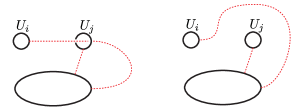
Figure 3.8. The given ribbon concordance $C$(left) and the new ribbon concordance $C^{\prime}$(right). Again, dotted red lines are the framed arcs along which we perform saddle moves.

Then the concordances $\overline{C^{\prime}}\circ C^{\prime}$ and $\bar{C}\circ C$ differ in the following way. In the movie of $\bar{C}\circ C$ drawn in Figure 3.6, denote the composition of the first two steps, i.e. births of $U_{1},\cdots,U_{n}$ followed by saddle moves from $K$ to $K\sqcup U_{1}^{\prime}\sqcup\cdots\sqcup U_{n}^{\prime}$, by $S_{1}$, and denote the composition of the rest by $S_{2}$. Furthermore, denote the self-concordance of $K\sqcup(\sqcup U_{k})\sqcup(\sqcup U_{k}^{\prime})$ given by the “neck-passing” of $U_{i}^{\prime}$ through $U_{j}$ by $S_{ij}$. Then we have

$$\bar{C}\circ C =S_{2}\circ S_{1},$$

$$\overline{C^{\prime}}\circ C^{\prime} =S_{2}\circ\overline{S_{ij}}\circ S_{1},$$

where we have assumed without loss of generality that $a_{i}$ and $D_{j}$ intersect positively at $p$. Now choose any $x\in F(K)$. Then, under the multiplicativity isomorphism

$$F(K\sqcup(\sqcup U_{k})\sqcup(\sqcup U_{k}^{\prime}))\xrightarrow{\sim}\left(F(K)\otimes\left(\bigotimes_{k\neq j}F(U_{i})\right)\otimes\left(\bigotimes_{k\neq i}F(U_{i}^{\prime})\right)\right)\otimes F(U_{i}^{\prime})\otimes F(U_{j}),$$

we have $F(S_{1})(x)=\sum_{m}x_{m}^{\prime}\otimes y_{m}\otimes u$ for some $x_{m}^{\prime}\in F(K)\otimes\left(\bigotimes_{k\neq j}F(U_{i})\right)\otimes\left(\bigotimes_{k\neq i}F(U_{i}^{\prime})\right)$ and $y_{m}\in F(U_{i}^{\prime})$ by associativity. Then, by the functoriality of $F$ and the weak neck-passing relation, we have

$$F(S_{ij})(x_{m}^{\prime}\otimes y_{m}\otimes u)=x_{m}^{\prime}\otimes F(S_{\phi})(y_{m}\otimes u)=x_{m}^{\prime}\otimes y_{m}\otimes u.$$

Hence $F(S_{ij}\circ S_{1})(x)=F(S_{ij})(F(S_{1})(x))=F(S_{1})(x)$, which implies $F(\overline{S_{ij}}\circ S_{1})=F(S_{1})$ by functoriality. But then we have

$$F(\overline{C^{\prime}}\circ C^{\prime})=F(S_{2})\circ F(\overline{S_{ij}}\circ S_{1})=F(S_{2})\circ F(S_{1})=F(\bar{C}\circ C).$$

Also, we have $n(C^{\prime})=n(C)-1$ by the construction of $C^{\prime}$. Therefore we have $F(\bar{C})\circ F(C)=\text{id}$ by induction on $n(C)$; this proves Theorem 1 in the associative case.

3.3.3. The case when $F$ is Khovanov-like

We now consider the case when $F$ is Khovanov-like, but not necessarily associative. Then the proof in the associative case cannot be applied directly, since the observation $F(S_{1})(x)=\sum_{m}x_{m}^{\prime}\otimes y_{m}\otimes u$ relies on the associativity of $F$. However we can still prove the same observation using our new assumption.

Since $F$ is now Khovanov-like, the unit $u\in F(\text{unknot})$ spans the kernel of the death map $\epsilon$ by definition. Under the same notation as used in the proof of the associative case, consider the death cobordism $E_{j}$ of the link $K\sqcup(\sqcup U_{k})\sqcup(\sqcup U_{k}^{\prime})$. Then the cobordism $E_{j}\circ S_{1}$ contains a closed sphere which bounds a 3-ball in $S^{3}\times I$. Thus, by the multiplicativity of $F$, we get $F(E_{j})\circ F(S_{1})=0$. But again by the multiplicativity, under the isomorphism

$$F(K\sqcup(\sqcup U_{k})\sqcup(\sqcup U_{k}^{\prime}))\xrightarrow{\sim}\left(F(K)\otimes\left(\bigotimes_{k\neq j}F(U_{i})\right)\otimes\left(\bigotimes_{k\neq i}F(U_{i}^{\prime})\right)\right)\otimes F(U_{i}^{\prime})\otimes F(U_{j}),$$

the map $F(E_{j})$ is given by $\text{id}\otimes\text{id}\otimes\epsilon$. Therefore the observation $F(S_{1})(x)=\sum_{m}x_{m}^{\prime}\otimes y_{m}\otimes u$ is still holds in this case, and the rest of the proof is the same. This proves Theorem 1 in the Khovanov-like case.

3.4. Proofs of the corollaries 2 and 3

Finally, using Theorem 1, which was proved in the last subsection, we can now prove the Corollaries 2 and 3.

Proof of Corollary 2.

All conic strong Khovanov-Floer theories are multiplicative and Khovanov-like. So the corollary holds for all conic strong Khovanov-Floer theories.

For the case of Khovanov-Rozansky homology, it is proven in [ETW17] that Khovanov-Rozansky homology is a TQFT of links in $\mathbb{R}^{3}$. Moreover, that result was upgraded in [MWW19], which proves that it is actually a TQFT of links in $S^{3}$. Since Khovanov-Rozansky homology is multiplicative and associative by its definition, we see that it induces injective maps for ribbon concordances by Theorem 1. ∎

Proof of Corollary 3.

If two vector spaces $V,W$ over $\mathbb{F}$ admit linear injections $V\rightarrow W$ and $W\rightarrow V$, then $V\simeq W$. ∎

4. $\mathbb{Z}$-grading and the neck passing relation

4.1. Nicely graded conic strong Khovanov-Floer theories

Some strong Khovanov-Floer theories come with a $\mathbb{Z}$-grading. We will say that a conic strong Khovanov-Floer theory $F$ is nicely graded if it carries a $\mathbb{Z}$-grading such that the cobordism maps for $F$ are degree-preserving up to some degree shift, and that $F(\text{unknot})$ is not concentrated in one grading. In such cases, we can get a relation which is much stronger than the weak neck-passing relation.

Note that we have an isomorphism of graded vector spaces

$$F(\text{unknot})\simeq\mathbb{F}[X]/(X^{2}),$$

which maps to unit $u$ to $1$; the counit $\epsilon:F(\text{unknot})\rightarrow\mathbb{F}$ is given by sending $1$ to $0$ and $X$ to $1$. With respect to such an identification, the assumption that $F$ is nicely graded is equivalent to assuming that the unit $1$ and the element $X$ lie in different gradings.

Consider the two-component unknot $U_{2}=A\sqcup B$ and define $S_{\phi}$ as in the previous section. Then we have the following theorem.

Theorem 12 (Neck-passing relation).

Let $F$ be a nicely graded conic strong Khovanov-Floer theory. Then $F(S_{\phi})=\text{id}$.

Proof.

Consider the birth cobordism $B_{A}$ for the component A, i.e. cobordism given by

$$B_{A}=(\text{birth for }A)\cup(\text{cylinder for }B).$$

Then $B_{A}$ is an oriented link cobordism from $B$ to $U_{2}$, and we have $F(B_{A})(1)=X\otimes 1$, where we are taking the identification

$$F(U_{2})\simeq\mathbb{F}[X]/(X^{2})\otimes\mathbb{F}[X]/(X^{2}),$$

and the first component in the tensor product corresponds to the component $A$ of $U_{2}$. But then $S_{\phi}\circ B_{A}$ is isotopic to $B_{A}$, so we have

$$F(S_{\phi})(1\otimes X)=F(S_{\phi})(F(B_{A})(1))=F(S_{\phi}\circ B_{A})(1)=F(B_{A})(1)=1\otimes X,$$

so the map $F(S_{\phi})$ fixes $1\otimes X$. Similarly, we can see that $F(S_{\phi})$ also fixes $1\otimes 1$.

By the weak neck-passing relation, we already know that $F(S_{\phi})$ also fixes $X\otimes 1$. Thus it remains to prove that $F(S_{\phi})(X\otimes X)=X\otimes X$. By the assumption that $F$ is nicely graded, we know that the $2\cdot\mathbf{gr}(X)$-graded piece of $F(U_{2})$ has rank $1$, generated by $X\otimes X$. Also, we know that the grading shift of $F(S_{\phi})$ is $0$ by the weak neck-passing relation. Thus we already know that $F(S_{\phi})(X\otimes X)=c\cdot X\otimes X$ for some scalar $c\in\mathbb{F}$. However, using the “upside-down” version of our argument, we can prove that $c=1$ as follows:

$$c=F(\overline{B_{A}})(c\cdot X\otimes X)=F(\overline{B_{A}}\circ S_{\phi})(X\otimes X)=F(\overline{B_{A}})(X\otimes X)=X.$$

Therefore we deduce that $F(S_{\phi})=\text{id}$. ∎

Using the above theorem, we can actually prove a stronger statement, although it will not be used in this paper. Let $L_{0}$ be a link and $L=L_{0}\sqcup U$, where $U$ is an unknot. Choose any component $K\subset L_{0}$, and a meridian $m$ of $K$. Then we can consider the self-isotopy $\phi_{L_{0},K}$ of $L$ defined by moving $U$ along $m$. As in the neck-passing relation, we can consider the link cobordism $S_{L_{0},K}$, defined as

$$S_{L_{0},K}=\bigcup_{t\in I}(\phi_{t}(L)\times\{t\})\subset S^{3}\times I.$$

Then, for any link TQFT $F$, we can consider the morphism $F(S_{L_{0},K})$.

Corollary 13 (Strong neck-passing relation).

Let $F$ be a nicely graded conic strong Khovanov-Floer theory. Then for any choice of $L_{0}$ and $K$, the map $F(S_{L_{0},K})$ is the identity.

Proof.

Consider the saddle cobordism with respect to an arc $a$ satisfying the following conditions:

• $a$ is interior-disjoint from $L$, and its boundary points $p,q$ lie on $K$, at which $a$ is transverse to $K$.

• Taking saddle of $L\cup m$, where $m$ is a meridian of $K$, along $a$, gives the link $L\cup\text{(Hopf link})$.

Then the saddle cobordism $S_{a}$ from $L$ to $L\cup\text{unknot}$ admits a left inverse, which is the death cobordism of the newly created unknot component. Thus $F(S_{a})$ is injective.

Now consider the following diagram.

Since $S_{L_{0}\cup U,U}\circ S_{a}$ is isotopic to $S_{a}\circ S_{L_{0},K}$, we get the following commutative square. Note that the square on the right side is due to the multiplicativity of $F$.

But we already know that $F(S_{U,U})$ is the identity. Therefore, by the injectivity of $F(S_{a})$, we deduce that $F(S_{L_{0},K})=\text{id}$. ∎

4.2. Knot Floer homology

The above proof cannot be used directly to prove that ribbon concordances induce injective maps between knot Floer homology, because of the following reasons:

• Knot Floer homology is not a TQFT of links and link cobordisms, but rather a TQFT of decorated links and decorated link cobordisms.

• Knot Floer homology is a reduced theory, i.e. we have a natural splitting

  $$HFK^{\circ}(L_{1}\sqcup L_{2},P_{1}\sqcup P_{2})\simeq HFK^{\circ}(L_{1},P_{1})\otimes HFK^{\circ}(L_{2},P_{2})\otimes V$$

  where $\circ$ is either hat or minus flavor and and $V=\mathbb{F}^{2}$.

Here, we recall that a decorated link is a link together with $z$-basepoints and $w$-basepoints which occur in alternating way, so that each component has at least two basepoints. Also, decorated link cobordism is a splitting of a given cobordism into two subsurfaces such that one contains all $z$-basepoints and the another contains all $w$-basepoints. For more details, see [JM18] and [Zem19b].

Now consider the 2-component unknot $U_{2}$, together with the decoration $P$, so that each component of $U_{2}$ has one $z$-basepoint and $w$-basepoint. Then we can construct a decoration $P_{\phi}$ on the “go-around” cobordism $S_{\phi}$ from $U_{2}$ to itself, so that for each cylinder component $C\subset S_{\phi}$, the decoration $P_{\phi}|_{C}$ is given by Figure 4.1.

Figure 4.1. The decoration $P_{\phi}$ on the cylinder component $C$.

Of course, the decoration $P_{\phi}$ on $S_{\phi}$ is not uniquely defined. However we can choose one anyway, which will give us a map

$$HFK^{\circ}(S_{\phi},P_{\phi})\,:\,HFK^{\circ}(U_{2},P)\rightarrow HFK^{\circ}(U_{2},P),$$

and this map is an automorphism because the decorated cobordism $(S_{\phi},P_{\phi})$ obviously has an inverse.

Now, when $\circ=\text{hat}$, then we have

$$\widehat{HFK}(U_{2},P)\simeq\mathbb{F}[\frac{1}{2}]\oplus\mathbb{F}[-\frac{1}{2}],$$

and when $\circ=\text{minus}$, we have

$$HFK^{-}(U_{2},P)\simeq\mathbb{F}[U][\frac{1}{2}]\oplus\mathbb{F}[U][-\frac{1}{2}].$$

In either case, the only Maslov grading-preserving automorphism of $HFK^{\circ}(U_{2},P)$ , where $\circ$ is either the minus or hat flavor, is the identity. Furthermore, the only automorphism of $\widehat{HFK}(U_{2},P)$ which has a constant grading shift is the identity, which has zero grading shift. Hence, in either hat-flavor or minus-flavor, the grading shift of $HFK^{\circ}(S_{\phi},P_{\phi})$ is zero, and thus we have

$$HFK^{\circ}(S_{\phi},P_{\phi})=\text{id}.$$

Therefore, by repeating our proof in the previous section, but now using the splitting formula

$$HFK^{\circ}(L_{1}\sqcup L_{2},P_{1}\sqcup P_{2})\simeq HFK^{\circ}(L_{1},P_{1})\otimes HFK^{\circ}(L_{2},P_{2})\otimes V$$

for knot Floer homology, together with the splitting formula for disjoint unions of cobordisms, given by

$$HFK^{\circ}(S_{1}\sqcup S_{2},P_{S_{1}}\sqcup P_{S_{2}})=HFK^{\circ}(S_{1},P_{S_{1}})\otimes HFK^{\circ}(S_{2},P_{S_{2}})\otimes\text{id}_{V},$$

we deduce that every ribbon concordance induces an injective map between $HFK$, in both hat- and minus-flavor.

Remark 14.

Using the arguments in the last section to knot Floer homology, we can easily see that neck-passing relation and strong neck-passing relation hold for knot Floer homology. Of course we should choose a decoration on our link cobordisms as in Figure 4.1.

5. $\widehat{HF}$ of the branched double cover

5.1. An alternative proof of the injectivity of $HF^{\circ}\circ\Sigma$ for hat- and minus-flavors

Consider the Heegaard Floer homology of the double branched cover, defined as the link TQFT

$$L\subset S^{3}\mapsto HF^{\circ}(\Sigma(L)),$$

where we take the flavor $\circ$ to be either hat or minus. Then the resulting TQFT satisfies functoriality for link cobordisms, defined by

$$\text{cobordism }S\mapsto\text{map }F_{\Sigma(S)}^{\circ},$$

but this carries a similar problem as in the case of knot Floer homology.

To be precise, the problem is the following. Although the assignment $L\mapsto HF^{\circ}(\Sigma(L)\sharp(S^{1}\times S^{2}))$ is a (unreduced) conic strong Khovanov-Floer theory, the assignment $L\mapsto HF^{\circ}(\Sigma(L))$ is not, since it satisfies a reduced version of multiplicativity

$$HF^{\circ}(\Sigma(L_{1}\sqcup L_{2}))\simeq HF^{\circ}(\Sigma(L_{1}))\otimes HF^{\circ}(\Sigma(L_{2}))\otimes V,$$

where the isomorphism is again natural with respect to cobordism maps. However, since we have

$$HF^{\circ}(\Sigma(U_{2}))\simeq HF^{\circ}(S^{1}\times S^{2}),$$

the only degree-preserving automorphism of $HF^{\circ}(\Sigma(U_{2}))$ is the identity. Thus, using the same argument used in the knot Floer case, we see that $\widehat{HF}\circ\Sigma$ satisfies the neck-passing relation. Therefore, for any ribbon concordance $C:K_{1}\rightarrow K_{2}$, the cobordism map $F_{\Sigma(C)}^{\circ}$ is injective, as already shown in [LVVW19] using a different method.

5.2. Involutions on $\widehat{HF}(\Sigma(K))$

Since $F_{\Sigma(\bar{C})}^{\circ}F_{\Sigma(C)}^{\circ}=\text{id}$ by the neck-passing relation, we actually know that $F_{\Sigma(C)}^{\circ}$ induces an inclusion of $HF^{\circ}(\Sigma(K_{1}))$ in $HF^{\circ}(\Sigma(K_{2}))$ in a way that it becomes a direct summand. This gives a very strong restriction on the deck transformation action(which we will denote as $\tau$) and the $\iota$-involution(which arises naturally in the construction of involutive Floer homology in [HM⁺17]) on $HF^{\circ}(\Sigma(K_{1}))$ when $K_{2}$ satisfies some nice conditions.

We briefly recall the definition of the two involutions $\tau$ and $\iota$. By the naturality of Heegaard Floer theory, due to Juhasz and Thurston[JTZ12], for any 3-manifold $M$ with a basepoint $z$, the pointed mapping class group $\mathbf{Mod}(M,z)$ acts on $\widehat{HF}(M)$. When $M=\Sigma(K)$ and $z\in K$, the deck transformation of $\Sigma(K)\rightarrow S^{3}$ fixes $z$, thus gives a $\mathbb{Z}_{2}$-action $\tau$ on $\widehat{HF}(M)$.

The involution $\iota$ is defined in a much more subtle way. Choose any Heegaard diagram $(\Sigma,\boldsymbol{\alpha},\boldsymbol{\beta},z)$ representing $\Sigma(K)$. Then we have the identity map

$$\text{id}:\widehat{CF}(\Sigma,\boldsymbol{\alpha},\boldsymbol{\beta},z)\rightarrow\widehat{CF}(\bar{\Sigma},\boldsymbol{\beta},\boldsymbol{\alpha},z),$$

and since both $(\Sigma,\boldsymbol{\alpha},\boldsymbol{\beta},z)$ and $(\bar{\Sigma},\boldsymbol{\beta},\boldsymbol{\alpha},z)$ represent $\Sigma(K)$, we have a naturality map

$$f:\widehat{CF}(\bar{\Sigma},\boldsymbol{\beta},\boldsymbol{\alpha},z)\rightarrow\widehat{CF}(\Sigma,\boldsymbol{\alpha},\boldsymbol{\beta},z),$$

which is defined uniquely up to chain homotopy. Then $f\circ\text{id}$ is a homotopy involution, so the induced automorphism on $\widehat{HF}(\Sigma(K))$ is a uniquely determined involution, which we denote as $\iota$.

As shown in [AKS19], the behaviors of two involutions $\tau$ and $\iota$ of $\widehat{HF}(\Sigma(K))$ are a bit different: sometimes they are identical, whereas sometimes they are not. To be precise, we know the following:

• When $K$ is quasi-alternating, then $\tau$ and $\iota$ are both trivial.

• When $K$ is an odd torus knot, then $\tau$ is trivial, but $\iota$ is nontrivial in general.

• When $K$ is a Montesinos knot, then $\tau=\iota$.

Note that, in the Montesinos case, there exists a $\iota$-invariant basis of $\widehat{HF}(\Sigma(K))$ such that the action of $\iota$ leaves exactly one basis element fixed, as shown in [DM17]. Furthermore, it is straightforward to see that $\tau$ and $\iota$ always commute, i.e. $\tau\circ\iota=\iota\circ\tau$. Using these results, we can now prove Theorem 4.

Proof of Theorem 4.

Suppose that $K_{0}$ is ribbon concordant to $K_{1}$ by a ribbon concordance $C$, and let $\sigma$ denote an involution, which is either $\tau$, $\iota$, or $\tau\circ\iota$. Then the involution $\sigma$ gives $\mathbb{F}[\mathbb{Z}_{2}]$-module structures on $\widehat{HF}(\Sigma(K_{0}))$ and $\widehat{HF}(\Sigma(K_{1}))$. Furthermore, the cobordism map $\hat{F}_{\Sigma(C)}$ commutes with $\sigma$ (since it commutes with both $\tau$ and $\iota$; see [AKS19] and [HM⁺17]), and $\hat{F}_{\Sigma(\bar{C})}\hat{F}_{\Sigma(C)}=\text{id}$, so $\widehat{HF}(\Sigma(K_{0}))$ is a $\mathbb{F}[\mathbb{Z}_{2}]$-module direct summand of $\widehat{HF}(\Sigma(K_{1}))$.

But it is obvious that every finitely generated $\mathbb{F}[\mathbb{Z}_{2}]$-module $M$ can be uniquely represented as

$$M=\mathbb{F}^{m_{M}}\oplus(\mathbb{F}\cdot v\oplus\mathbb{F}\cdot\sigma(v))^{n_{M}},$$

so that if an $\mathbb{F}[\mathbb{Z}_{2}]$-module $M$ is a direct summand of $N$, then $m_{M}\leq m_{N}$ and $n_{M}\leq n_{N}$. This proves the theorem. ∎

References

- [AKS19] Antonio Alfieri, Sungkyung Kang, and Andras I Stipsicz, Connected Floer homology of covering involutions, arXiv preprint arXiv:1905.11613 (2019).
- [BHL19] John A Baldwin, Matthew Hedden, and Andrew Lobb, On the functoriality of Khovanov–Floer theories, Advances in Mathematics 345 (2019), 1162–1205.
- [DM17] Irving Dai and Ciprian Manolescu, Involutive Heegaard Floer homology and plumbed three-manifolds, Journal of the Institute of Mathematics of Jussieu (2017), 1–41.
- [ETW17] Michael Ehrig, Daniel Tubbenhauer, and Paul Wedrich, Functoriality of colored link homologies, arXiv preprint arXiv:1703.06691 (2017).
- [Gor81] C McA Gordon, Ribbon concordance of knots in the 3-sphere, Mathematische Annalen 257 (1981), no. 2, 157–170.
- [HM+17] Kristen Hendricks, Ciprian Manolescu, et al., Involutive Heegaard Floer homology, Duke Mathematical Journal 166 (2017), no. 7, 1211–1299.
- [JM18] András Juhász and Marco Marengon, Computing cobordism maps in link Floer homology and the reduced Khovanov TQFT, Selecta Mathematica 24 (2018), no. 2, 1315–1390.
- [JMZ19] András Juhász, Maggie Miller, and Ian Zemke, Knot cobordisms, torsion, and floer homology, arXiv preprint arXiv:1904.02735 (2019).
- [JTZ12] András Juhász, Dylan P Thurston, and Ian Zemke, Naturality and mapping class groups in Heegaard Floer homology, arXiv preprint arXiv:1210.4996 (2012).
- [Kho99] Mikhail Khovanov, A categorification of the Jones polynomial, arXiv preprint math/9908171 (1999).
- [KM11] Peter B Kronheimer and Tomasz S Mrowka, Khovanov homology is an unknot-detector, Publications mathématiques de l’IHÉS 113 (2011), no. 1, 97–208.
- [KR04] Mikhail Khovanov and Lev Rozansky, Matrix factorizations and link homology, arXiv preprint math/0401268 (2004).
- [LVVW19] Tye Lidman, David Shea Vela-Vick, and C-M Michael Wong, Heegaard Floer homology and ribbon homology cobordisms, arXiv preprint arXiv:1904.09721 (2019).
- [LZ19] Adam Simon Levine and Ian Zemke, Khovanov homology and ribbon concordance, arXiv preprint arXiv:1903.01546 (2019).
- [MWW19] Scott Morrison, Kevin Walker, and Paul Wedrich, Invariants of 4-manifolds from Khovanov-Rozansky link homology, arXiv preprint arXiv:1907.12194 (2019).
- [OS05] Peter Ozsváth and Zoltán Szabó, On the Heegaard Floer homology of branched double-covers, Advances in Mathematics 194 (2005), no. 1, 1–33.
- [Ras10] Jacob Rasmussen, Khovanov homology and the slice genus, Inventiones mathematicae 182 (2010), no. 2, 419–447.
- [Sal17] Adam Saltz, Strong Khovanov-Floer theories and functoriality, arXiv preprint arXiv:1712.08272 (2017).
- [Sar19] Sucharit Sarkar, Ribbon distance and khovanov homology, arXiv preprint arXiv:1903.11095 (2019).
- [Sza10] Zoltán Szabó, A geometric spectral sequence in Khovanov homology, arXiv preprint arXiv:1010.4252 (2010).
- [Zem15] Ian Zemke, A graph TQFT for hat heegaard floer homology, arXiv preprint arXiv:1503.05846 (2015).
- [Zem19a] by same author, Knot Floer homology obstructs ribbon concordance, arXiv preprint arXiv:1902.04050 (2019).
- [Zem19b] by same author, Link cobordisms and functoriality in link Floer homology, Journal of Topology 12 (2019), no. 1, 94–220.