Periodic solutions of one-dimensional cellular automata with random rules

Abstract

We study cellular automata with randomly selected rules. Our setting are two-neighbor rules with a large number $n$ of states. The main quantity we analyze is the asymptotic probability, as $n\to\infty$, that the random rule has a periodic solution with given spatial and temporal periods. We prove that this limiting probability is non-trivial when the spatial and temporal periods are confined to a finite range. The main tool we use is the Chen-Stein method for Poisson approximation. The limiting probability distribution of the smallest temporal period for a given spatial period is deduced as a corollary and relevant empirical simulations are presented.

1 Introduction

We investigate one-dimensional cellular automata (CA), a class of temporally and spatially discrete dynamical systems, in which the update rule is selected at random. Our focus is the asymptotic behavior of the probability that such random CA has a periodic solution with fixed spatial and temporal periods, as $n$, the number of states, goes to infinity. This complements the work in [7], where the limiting behavior of the longest temporal period with a given spatial period is explored. We assume the simplest nontrivial setting of two-neighbor rules.

The (spatial) configuration at time $t$ of a one-dimensional CA with number of states $n$ is a function $\xi_{t}$ that assigns to every site $x\in\mathbb{Z}$ its state $\xi_{t}(x)\in\mathbb{Z}_{n}=\{0,1,\dots,n-1\}$. The evolution of spatial configurations is given by a local 2-neighbor rule $f:\mathbb{Z}_{n}^{2}\to\mathbb{Z}_{n}$ that updates $\xi_{t}$ to $\xi_{t+1}$ as follows:

$$\xi_{t+1}(x)=f(\xi_{t}(x-1),\xi_{t}(x)),\quad\text{for all }x\in\mathbb{Z}.$$

We abbreviate $f(a,b)=c$ as $a\underline{b}\mapsto c$. We give a rule by listing its values for all pairs in reverse alphabetical order, from $(n-1,n-1)$ to $(0,0)$.

Given $\xi_{0}$, the update rule determines the trajectory $\xi_{t}$, $t\in\mathbb{Z}_{+}=\{0,1,\ldots\}$, or, equivalently, the the space-time configuration, which is the map $(x,t)\mapsto\xi_{t}(x)$ from $\mathbb{Z}\times\mathbb{Z}_{+}$ to $\mathbb{Z}_{n}$. By convention, a picture of this map is a painted grid, in which the temporal axis is oriented downward, the spatial axis is oriented rightward, and each state is given as a different color. To give an example, a piece of the space-time configuration is presented in Figure 1. In this figure, we have three states, i.e., $n=3$, and the rule is 021102022, i.e., $2\underline{2}\mapsto 0,2\underline{1}\mapsto 2,2\underline{0}\mapsto 1,1\underline{2}\mapsto 1,1\underline{1}\mapsto 0,1\underline{0}\mapsto 2,0\underline{2}\mapsto 0,0\underline{1}\mapsto 2$ and $0\underline{0}\mapsto 2$.

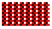
Figure 1: A piece of the space-time configuration of a 3-state rule. In the space-time configuration, 0, 1 and 2 are represented by white, red and black cells, respectively.

The space-time configuration in Figure 1 exhibits periodicity in both space and time. In the literature [3], such a configuration is called doubly or jointly periodic. Since these are the only objects we study, we simply refer to such a configuration as a periodic solution (PS). To be precise, start with a periodic spatial configuration $\xi_{0}$, such that there is a $\sigma>0$ satisfying $\xi_{0}(x)=\xi_{0}(x+\sigma)$, for all $x\in\mathbb{Z}$. Run a CA rule $f$ starting with $\xi_{0}$. If we have $\xi_{\tau}(x)=\xi_{0}(x)$, for all $x\in\mathbb{Z}$ and that $\sigma$ and $\tau$ are both minimal, then we have found a periodic solution of temporal period $\tau$ and spatial period $\sigma$. A tile is any rectangle with $\tau$ rows and $\sigma$ columns within this space-time configuration. We interpret a tile as a configuration on a discrete torus; we will not distinguish between spatial and temporal translations of a PS, and therefore between either rotations of a tile. The tile of a PS is by definition unique and we will identify a PS with its tile. As an example, in Figure 1, we start with the initial configuration $\xi_{0}=120^{\infty}=\dots 120120120\dots$ (we give a configuration as a bi-infinite sequence when the position of the origin is clear or unimportant). After 2 updates, we have $\xi_{2}(x)=\xi_{0}(x)$, for all $x\in\mathbb{Z}$, thus the PS has temporal period 2 and spatial period 3. Its tile is $\begin{matrix}1&2&0\\ 2&1&1\\ \end{matrix}$ .

CA that exhibit temporally periodic or jointly periodic behavior have been explored to some degree in the literature, and we give a brief review of some highlights. The foundational work is commonly considered to be [13]. This paper, together with its successors [9, 10], focuses on algebraic methods to investigate additive CA, but also lays the foundation for more general rules. More recent papers on temporal periodicity of additive binary rules include [4] and [14]. The literature on non-additive rules is more scarce, but includes notable works [3] and [2] on the density of periodic configurations, which use both rigorous and experimental methods. A method of finding temporally periodic trajectories is discussed in [20], which reiterates the utility of the relation between periodic configurations and cycles on graphs induced by the CA rules, introduced in [13]. This approach is useful in the present paper as well. Papers investigating long temporal periods of CA also include [17, 16], as well as our companion papers [7, 6]. To mention another take on periodicity, the paper [5] introduces robust PS, which are those that expand into any environment with positive speed, and investigates their existence in all range 2 (i.e., 3-neighbor) binary CA.

We now present a formal setting to investigate PS from random rules, which, to our knowledge, have not been explored before. Our rule space $\Omega_{n}$ consists of $n^{n^{2}}$ rules and we assign a uniform probability $\mathbb{P}$ to each rule $f$, therefore $\mathbb{P}(\{f\})=1/n^{n^{2}}$. Let $\mathcal{P}_{\tau,\sigma,n}$ be the random set of PS with temporal period $\tau$ and spatial period $\sigma$ of such a randomly chosen CA rule. The main quantity we are interested in is $\lim\mathbb{P}\left(\mathcal{P}_{\tau,\sigma,n}\neq\emptyset\right)$ as $n\to\infty$ for a fixed pair of $(\tau,\sigma)$. In words, our focus is the limiting probability that a random CA rule has a PS with given temporal and spatial periods. In the following theorem, we prove that this limit is nontrivial for any $\tau$ and $\sigma$. Define

(1) $$\lambda_{\tau,\sigma}=\frac{1}{\tau\sigma}\sum_{d\bigm{|}\gcd(\tau,\sigma)}\varphi(d)d,$$

where $\varphi$ the Euler totient function.

Theorem 1.

For any fixed integers $\tau\geq 1$ and $\sigma\geq 1$, $\mathbb{P}\left(\mathcal{P}_{\tau,\sigma,n}\neq\emptyset\right)\to 1-\exp\left(-\lambda_{\tau,\sigma}\right)$ as $n\to\infty$.

We also prove a more general result concerns the number of PS with a range of periods. Assume $\mathcal{T},\Sigma\subset\mathbb{N}=\{1,2,\dots\}$, and define $\mathcal{P}_{\mathcal{T},\Sigma,n}=\mathcal{P}_{\mathcal{T},\Sigma,n}(f)=\bigcup_{(\tau,\sigma)\in\mathcal{T}\times\Sigma}\mathcal{P}_{\tau,\sigma,n}$ and

(2) $$\lambda_{\mathcal{T},\Sigma}=\sum_{(\tau,\sigma)\in\mathcal{T}\times\Sigma}\lambda_{\tau,\sigma}.$$

Theorem 2.

For a finite $\mathcal{T}\times\Sigma\subset\mathbb{N}\times\mathbb{N}$, $\mathbb{P}\left(\mathcal{P}_{\mathcal{T},\Sigma,n}\neq\emptyset\right)\to 1-\exp\left(-\lambda_{\mathcal{T},\Sigma}\right)$ as $n\to\infty$.

We define the random variable

$$Y_{\sigma,n}=\min\{\tau:\mathcal{P}_{\tau,\sigma,n}\neq\emptyset\}$$

to be the smallest temporal period of a PS with spatial period $\sigma$ of a randomly selected $n$-state rule. Figure 2 provides four examples of rules $f$, with $Y_{4,3}(f)=1,2,3$ and $4$. As a consequence of Theorem 2, for a given $\sigma>0$, the random variable $Y_{\sigma,n}$ is stochastically bounded, in the sense of the following corollary.

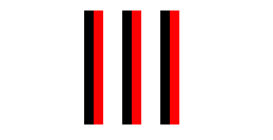
(a) 012200210

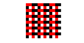
(b) 021102120

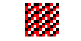
(c) 100112122

(d) 101201021

Figure 2: Pieces of PS for $\sigma=4$ and 3-state rules, 012200210, 021102120, 100112122 and 101201021, with temporal period $\tau=1,2,3$ and $4$, respectively. (See the discussion before Corollary 4.) These temporal periods are the smallest in each case, as verified by Algorithm 2.5 in Section 2.3. Algorithm 2.8 in Section 2.4 shows that $\sigma=4$ is not the minimal spatial period of PS given the corresponding temporal period $\tau=1,2$ and $3$ in the first three rules, while for the last rule $\sigma=4$ is also the minimal spatial period of PS for temporal period $\tau=4$.

Corollary 3.

The random variable $Y_{\sigma,n}$ converges weakly to a nontrivial distribution as $n\to\infty$.

We now briefly discuss the relation between this corollary and the main results of [7] and [6]. In [7], we consider a more general setting of CA rules with $r$ neighbors, that is, $\xi_{t}$ updates to $\xi_{t+1}$ according to the rule $f:\mathbb{Z}_{n}^{r}\to\mathbb{Z}_{n}$, so that

$$\xi_{t+1}(x)=f(\xi_{t}(x-r+1),\dots,\xi_{t}(x)),\quad\text{for all }x\in\mathbb{Z}.$$

Fix a spatial period $\sigma$ and an $r$. Let $X_{\sigma,n}=\max\{\tau:\mathcal{P}_{\tau,\sigma,n}\neq\emptyset\}$ be the largest temporal period of a PS with spatial period $\sigma$ of a randomly selected $r$-neighbor rule. In the case when $\sigma\leq r$, we prove that $X_{\sigma,n}/n^{\sigma/2}$ converges in distribution to a nontrivial limit, as $n\to\infty$. We also provide empirical evidence that the same result holds when $\sigma>r$, although in that case we do not have a rigorous proof even for $r=2$. At least for $r=\sigma=2$, therefore, the shortest temporal period is stochastically bounded while the longest is on the order of $n$. Moreover, it is not hard to see that the maximum of the random variable $Y_{2,n}$ and $X_{2,n}$ are both $n^{2}-n$. More generally, in [6] and [12], we construct rules $f$ with $Y_{\sigma,n}(f)\geq C(\sigma)n^{\sigma}$. That is, the maximum of the random variable $Y_{\sigma,n}$ is of the same order as its upper bound $n^{\sigma}-\mathcal{O}(n^{\sigma/2})$, guaranteed by the pigeonhole principle.

In the next section, we collect our main tools: tiles of PS; circular shifts; oriented graphs induced by a rule; and the Chen-Stein method. In Section 3, we discuss a class of tiles that plays a central role. We prove the main results in Section 4 and conclude with a discussion and several unsolved problems in Section 5.

2 Preliminaries

2.1 Tiles of a PS

We recall that the spatial and temporal periods $\sigma$ and $\tau$ are assumed to be minimal, so a tile cannot be divided into smaller identical pieces. We now take a closer look into properties of tiles.

If we choose an element in a tile $T$ to be placed at the position $(0,0)$, $T$ may be expressed as a matrix $T=(a_{i,j})_{i=0,\dots,\tau-1,j=0,\dots,\sigma-1}$. We always interpret the two subscripts modulo $\tau$ and $\sigma$. The matrix is determined up to a space-time rotation, but note that two different rotations cannot produce the same matrix due to the minimality of $\sigma$ and $\tau$. We say that $a_{i,j}$ is an element in $T$, and write $a_{i,j}\in T$, when we want to refer to the element of the matrix at the position $(i,j)$, and use the notation $\mathtt{row}_{i}$ and $\mathtt{col}_{j}$ to denote the $i$th row and $j$th column of a tile $T$, again after we fix $a_{0,0}$. All the properties we now introduce are independent of the chosen rotation (as they must be, to be meaningful).

Let $T_{1}$ and $T_{2}$ be two tiles and $a_{i,j}$, $b_{k,m}$ be elements in $T_{1}$ and $T_{2}$, respectively. We say that $T_{1}$ and $T_{2}$ are orthogonal, and denote this property by $T_{1}\perp T_{2}$, if $\left(a_{i,j},a_{i,j+1}\right)\neq\left(b_{k,m},b_{k,m+1}\right)$ for $i,j,k,m\in\mathbb{Z}_{+}$. It is important to observe that in this case the two assignments $a_{i,j}\underline{a_{i,j+1}}\mapsto a_{i+1,j+1}$ is and $b_{k,m}\underline{b_{k,m+1}}\mapsto b_{k+1,m+1}$ occur independently.

We say that $T_{1}$ and $T_{2}$ are disjoint, and denote this property by $T_{1}\cap T_{2}=\emptyset$, if $a_{i,j}\neq b_{k,m}$, for $i,j,k,m\in\mathbb{Z}_{+}$. Clearly, every pair of disjoint tiles is orthogonal, but not vice versa.

Let $s(T)=\#\{a_{i,j}:a_{i,j}\in T\}$ be the number of different states in the tile. Furthermore, let $p(T)=\#\{(a_{i,j},a_{i,j+1}):a_{i,j},a_{i,j+1}\in T\}$ be the assignment number of $T$; this is the number of values of the rule $f$ specified by $T$. Clearly, $p(T)\geq s(T)$, so we define $\ell=\ell(T)=p(T)-s(T)$ to be the lag of $T$. We record a few immediate properties of a tile in the following Lemma.

Lemma 2.1.

Let $T=(a_{i,j})_{i=0,\dots,\tau-1,j=0,\dots,\sigma-1}$ be the tile of a PS with periods $\tau$ and $\sigma$. Then $T$ satisfies the following properties:

1. Uniqueness of assignment: if $(a_{i,j},a_{i,j+1})=(a_{k,m},a_{k,m+1})$, then $a_{i+1,j+1}=a_{k+1,m+1}$.

2. Aperiodicity of rows: each row of $T$ cannot be divided into smaller identical pieces.

Proof.

Part 1 is clear since $T$ is generated by a CA rule. Part 2 follows from part 1 and the assumption that the spatial period of $T$ is minimal. ∎

By contrast, we remark that there may exist periodic columns in a tile of a PS. For example, note that the first column in Figure 2(d) has period $2$ rather than $4=\tau$.

2.2 Circular shifts

In this section, we introduce circular shifts, operation on $Z_{n}^{\sigma}$ (or $Z_{n}^{\tau}$), the set of words of length $\sigma$ (or $\tau$) from the alphabet $\mathbb{Z}_{n}$. They will be useful in Section 3.

Definition 2.2.

Let $\mathbb{Z}_{n}^{\sigma}$ consist of all length-$\sigma$ words. A circular shift is a map $\pi:\mathbb{Z}_{n}^{\sigma}\to\mathbb{Z}_{n}^{\sigma}$, given by an $i\in\mathbb{Z}_{+}$ as follows: $\pi(a_{0}a_{1}\dots a_{\tau-1})=a_{i}a_{i+1}\dots a_{i+\sigma-1}$, where the subscripts are modulo $\sigma$. The order of a circular shift $\pi$ is the smallest $k$ such that $\pi^{k}(A)=A$ for all $A\in\mathbb{Z}_{n}^{\sigma}$, and is denoted by $\text{\rm ord}(\pi)$. Circular shifts on $\mathbb{Z}_{n}^{\tau}$ will also appear in the sequel and are defined in the same way.

Lemma 2.3.

Let $\pi$ be a circular shift on $\mathbb{Z}_{n}^{\sigma}$ and let $A\in\mathbb{Z}_{n}^{\sigma}$ be an aperiodic length-$\sigma$ word from alphabet $\mathbb{Z}_{n}$. Then: (1) $\text{\rm ord}(\pi)\bigm{|}\sigma$; and (2) for any $d\bigm{|}\sigma$,

$$|\left\{B\in\mathbb{Z}_{n}^{\sigma}:A=\pi(B)\text{ for some }\pi\text{ with }\text{\rm ord}(\pi)=d\right\}|=\varphi(d).$$

Proof.

Note that the $\sigma$ circular shifts form a cyclic group of order $\sigma$. Moreover, $\text{\rm ord}(\pi)$ of a circular shift is its order in the group, thus (1) follows. To prove (2), observe that the circular shifts of order $d$ generate a cyclic subgroup and the number of them is $\varphi(d)$. As $A$ is aperiodic, the cardinality in the claim is the same. ∎

We say that two words $A$ and $B$ of length $\sigma$ are equal up to a circular shift if $B=\pi(A)$ for some circular shift $\pi$. For example, words $0123$ and $2301$ are not equal, but are equal up to a circular shift.

2.3 Directed graph on configurations

Connections between directed graphs on periodic configurations and cycles are well-established [13, 19, 11, 20], as they are useful for analysis of PS with a fixed spatial period.

Definition 2.4.

Let $A=a_{0}\dots a_{\sigma-1}$ and $B=b_{0}\dots b_{\sigma-1}$ be two words from alphabet $\mathbb{Z}_{n}$. We say that $A$ down-extends to $B$, if $f(a_{i},a_{i+1})=b_{i+1}$, for all $i\geq 0$, where (as usual) the indices are modulo $\sigma$.

If $A$ down-extends to $B$, then $\pi(A)$ also down-extends to $\pi(B)$, for any circular shift $\pi$ on $\mathbb{Z}_{n}^{\sigma}$. Therefore, we can define, for a fixed $\sigma$, the configuration digraph on equivalence classes of words equal up to circular shifts, which has an arc from $A$ to $B$ if $A$ down-extends to $B$ (where we identify the equivalence class with any of its representatives). See Figure 3 for the configuration digraph of the 3-state rule 021102022. For instance, there is an arc from 122 to 210 as $1\underline{2}\mapsto 1$, $2\underline{2}\mapsto 0$ and $2\underline{1}\mapsto 2$. The following algorithm and self-evident proposition determine the PS in Figure 1 from the length-2 cycle $120\leftrightarrow 211$ in Figure 3.

Algorithm 2.5.

Input: Configuration digraph $D_{\sigma,f}$ of $f$ and spatial period $\sigma$.
Step 1: Find all the directed cycles in $D_{\sigma,f}$.
Step 2: For each cycle $A_{0}\to A_{1}\to\cdots\to A_{\tau-1}\to A_{0}$, form the tile $T$ by placing configurations $A_{0},A_{1},\ldots,A_{\tau-1}$ on successive rows.
Step 3: If the spatial period of $T$ is minimal, output $T$.

Proposition 2.6.

All PS of spatial period $\sigma$ of $f$ are obtained by Algorithm 2.5.

We remark that Step 3 in Algorithm 2.5 is necessary, as, for instance, the cycle $000\leftrightarrow 222$ in Figure 3 results in a PS of spatial period 1 instead of 3. In the same vein, the periods of configurations are non-increasing, and may decrease, along any directed path on the configuration digraph. For example, in Figure 3, the configuration 100 down-extends to 222, thus the period is reduced from 3 to 1 and then remains 1. These period reductions play a crucial role in our companion paper [7].

Figure 3: Configuration digraph of the 3-state rule 021102022 and spatial period $\sigma=3$.

2.4 Directed graph on labels

In this subsection, we fix the temporal period $\tau$, instead of the spatial period $\sigma$, and obtain another digraph induced by the rule. The construction below is an adaption of label trees from [5]. We call such a graph label digraph.

Definition 2.7.

Let $A=a_{0}\dots a_{\tau-1}$ and $B=b_{0}\dots b_{\tau-1}$ be two words from alphabet $\mathbb{Z}_{n}$, which we call labels of length $\tau$. (While it is best to view them as vertical columns, we write them horizontally for reasons of space, as in [5].) We say that $A$ right-extends to $B$ if $f(a_{i},b_{i})=b_{i+1}$, for all $i\in\mathbb{Z}_{+}$, where (as usual) the indices are modulo $\tau$. We form the label digraph associated with a given $\tau$ by forming an arc from a label $A$ to a label $B$ if $A$ right-extends to $B$.

A label $A=a_{0}\dots a_{\tau-1}$ right-extends to $B$ if and only if we preserve the temporal periodicity from a column $A$ to the column $B$ to its right. This fact is the basis for the Algorithm 2.8 below, which gives all the PS with temporal period $\tau$. The label digraph of same rule as in Figure 3 and temporal period $\tau=2$ is presented in Figure 4. For example, we have the arc from label 12 to 10 as $1\underline{1}\mapsto 0$, $2\underline{0}\mapsto 1$. Either of the two 3-cycles in the digraph generates the PS in Figure 1.

Algorithm 2.8.

Input: Label digraph $D_{\tau,f}$ of $f$ with period $\tau$.
Step 1: Find all the directed cycles in $D_{\tau,f}$.
Step 2: For each cycle $A_{0}\to A_{1}\to\cdots\to A_{\sigma-1}\to A_{0}$, form the tile $T$ by placing configurations $A_{0},A_{1},\ldots,A_{\sigma-1}$ on successive columns.
Step 3: If both spatial and temporal periods of $T$ are minimal, then output $T$.

Proposition 2.9.

All PS of temporal period $\tau$ of $f$ can be obtained by the Algorithm 2.8.

Again, Step 3 is necessary due to the same reason as Section 2.3. However, note the differences between the two graphs: the out-degrees in Figure 4 are between $0$ and $3$, and the temporal periods are not necessarily non-decreasing along a directed path. For example, 00 right-extends to 02. We also note that lifting the label digraph to one on equivalence classes, although possible, makes cycles more obscure and is thus less convenient.

Figure 4: Label digraph of the 3-state rule 021102022 and temporal period $\tau=2$.

2.5 Chen-Stein method for Poisson approximation

The main tool we use to prove Poisson convergence is the Chen-Stein method [1]. We denote by $\text{\rm Poisson}(\lambda)$ a Poisson random variable with expectation $\lambda$, and by $d_{\text{TV}}$ the total variation distance. We need the following setting for our purposes. Let $I_{i}$, for $i\in\Gamma$ be indicators of a finite family of events, which is indexed by $\Gamma$, $p_{i}=\mathbb{E}(I_{i})$, $W=\sum_{i\in\Gamma}I_{i}$, $\lambda=\sum_{i\in\Gamma}p_{i}=\mathbb{E}W$, and $\Gamma_{i}=\{j\in\Gamma:j\neq i,\,I_{i}\text{ and }I_{j}\text{ are not independent}\}$. We quote Theorem 4.7 from [15].

Lemma 2.10.

We have

$$d_{\text{TV}}(W,\text{\rm Poisson}(\lambda))\leq\min(1,\lambda^{-1})\left[\sum_{i\in\Gamma}p_{i}^{2}+\sum_{i\in\Gamma,j\in\Gamma_{i}}\left(p_{i}p_{j}+\mathbb{E}\left(I_{i}I_{j}\right)\right)\right].$$

In our applications of the above lemma, all deterministic and random quantities depend on the number $n$ of states, which we make explicit by the subscripts. In our setting, we prove that $d_{\text{TV}}(W_{n},\text{\rm Poisson}(\lambda_{n}))=\mathcal{O}(1/n)$ and that $\lambda_{n}\to\lambda$ as $n\to\infty$, for an explicitly given $\lambda$, which implies that $W_{n}$ converges to $\text{\rm Poisson}(\lambda)$ in distribution. See Theorem 1 and Theorem 2.

3 Simple tiles

We call a tile $T$ simple if its lag vanishes: $\ell(T)=p(T)-s(T)=0$. It turns out that in $\mathbb{P}(\mathcal{P}_{\tau,\sigma,n}\neq\emptyset)$, the probability of existence of PS with simple tiles provides the dominant terms, thus this class of tiles is of central importance. For example, consider the tiles

$$T_{1}=\begin{matrix}0&1&2&3\\ 2&3&0&1\\ \end{matrix},\qquad T_{2}=\begin{matrix}0&1&2&1\\ 2&1&0&1\\ \end{matrix}.$$

Then $T_{1}$ is simple, as $s(T_{1})=p(T_{1})=4$, but $T_{2}$ is not, as $s(T_{2})=3$ and $p(T_{2})=4$. Naturally, we call a PS simple if its tile is simple.

We denote by $\mathcal{P}_{\tau,\sigma,n}^{(\ell)}$ as the set of PS whose tile $T$ has lag $\ell$. Thus the set of simple PS is $\mathcal{P}_{\tau,\sigma,n}^{(0)}$. The following lemma addresses ramifications of repeated states in simple tiles.

Lemma 3.1.

Assume $T=(a_{i,j})_{i=0,\dots,\tau-1,j=0,\dots,\sigma-1}$ is a simple tile. Then

1. the states on each row of $T$ are distinct;

2. if two rows of $T$ share a state, then they are circular shifts of each other;

3. the states on each column of $T$ are distinct; and

4. if two columns of $T$ share a state, then they are circular shifts of each other.

Proof.

Part 1: When $\sigma=1$, each row contains only one state, making the claim trivial. Now, assume that $\sigma\geq 2$ and that $a_{i,j}=a_{i,k}$ for some $i$ and $j\neq k$. We must have $a_{i,j+1}=a_{i,k+1}$ in order to avoid $p(T)>s(T)$. Repeating this procedure for the remaining states on $\mathtt{row}_{i}$ shows that this row is periodic, contradicting part 2 of Lemma 2.1.

Part 2: If $a_{i,j}=a_{k,m}$, for $i\neq k$, then the states to their right must agree, i.e., $a_{i,j+1}=a_{k,m+1}$, in order to avoid $p(T)>s(T)$. Repeating this observation for the remaining states on $\mathtt{row}_{i}$ and $\mathtt{row}_{k}$ gives the desired result.

Part 3: Assume a column contains repeated state, say $a_{i,j}=a_{k,j}$ for some $i,j$ and $k$. By part 2, $\mathtt{row}_{i}$ is exactly the same as $\mathtt{row}_{k}$, so that the temporal period of this tile can be reduced, a contradiction.

Part 4: Assume that $a_{i,j}=a_{k,m}$, for $j\neq m$. Then $a_{i,j+1}=a_{k,m+1}$ by parts 1 and 2. So, $a_{i+1,j+1}=a_{k+1,m+1}$ by part 1 in Lemma 2.1. So, $a_{i+1,j}=a_{k+1,m}$, again by parts 1 and 2. Now, repeating the previous step for $a_{i+1,j}=a_{k+1,m}$ gives the desired result. ∎

We revisit the remark following Lemma 2.1: a tile may have periodic columns, but such a tile cannot be simple.

Suppose a tile $T=(a_{i,j})_{i=0,\dots,\tau-1,j=0,\dots,\sigma-1}$ is simple. We will take a closer look with circular shifts of rows, so we fix a row, say the first row $\mathtt{row}_{0}$. (We could start with any row, but we pick the first one for concreteness.) Let

$$i=\min\{k=1,2,\dots,\tau-1:\mathtt{row}_{k}=\pi(\mathtt{row}_{0}),\text{ for some circular shift }\pi:\mathbb{Z}^{\sigma}\to\mathbb{Z}^{\sigma}\}$$

be the smallest $i$ such that $\mathtt{row}_{i}$ is a circular shift of $\mathtt{row}_{0}$, and let $i=0$ if and only if $T$ does not have circular shifts of $\mathtt{row}_{0}$ other than this row itself. Then this circular shift satisfies $\mathtt{row}_{(j+i)\mod\tau}=\pi(\mathtt{row}_{j})$, for all $j=0,\dots,\tau-1$ and $i$ is determined by the tile $T$; we denote this circular shift by $\pi_{T}^{r}$. We denote by $\pi_{T}^{c}$ the analogous circular shift for columns.

Lemma 3.2.

Let $T$ be a simple tile of a PS, and let $d_{1}=\text{ord }(\pi_{T}^{r})$ and $d_{2}=\text{ord }(\pi_{T}^{c})$. Then $d_{1}$ and $d_{2}$ are equal and divide $\gcd(\tau,\sigma)$.

Proof.

Fix an element as $a_{0,0}$. By Lemma 3.1, parts 1 and 2, $a_{0,0}$ appears in $d_{1}$ rows of $T$. It also appears in $d_{2}$ columns by Lemma 3.1, parts 3 and 4. As a consequence, $d_{1}=d_{2}$. The divisibility follows from Lemma 2.3. ∎

Lemma 3.3.

An integer $s\leq n$ is the number of states in a simple tile $T=(a_{i,j})_{i=0,\dots,\tau-1,j=0,\dots,\sigma-1}$ of PS if and only if there exists $d\bigm{|}\gcd(\tau,\sigma)$, such that $s=\tau\sigma/d$.

Proof.

Let $T=(a_{i,j})_{i=0,\dots,\tau-1,j=0,\dots,\sigma-1}$. Assume that $s(T)=s$ and let $d=\text{ord }(\pi_{T}^{r})$. Then by Lemma 3.1, parts 1 and 2, the first $\tau/d$ rows of $T$ contain all states that are in $T$. As a result, $s=\tau\sigma/d$ and $d=\text{ord }(\pi_{T}^{r})\bigm{|}\gcd(\tau,\sigma)$.

Now assume that $d\bigm{|}\gcd(\tau,\sigma)$. Then there exists a circular shift $\pi:\mathbb{Z}^{\sigma}\to\mathbb{Z}^{\sigma}$, such that $\text{ord }(\pi)=d$. To form a simple tile $T$ with $s(T)=\tau\sigma/d$ states, construct a rectangle of $\tau/d$ rows and $\sigma$ columns using $\tau\sigma/d$ different states in the first $\tau/d$ rows of $T$. Let $\mathtt{row}_{\tau/d}$ be defined by $\pi(\mathtt{row}_{0})$ and the subsequent rows are all automatically defined by the maps that are assigned in the first $\tau/d$ rows, by Lemma 2.1, part 1. ∎

The above lemma gives the possible values of $s(T)$ for a simple tile $T$ and the next one enumerates the number of simple tiles of PS containing $s$ different states.

Lemma 3.4.

The number of simple tiles of PS with temporal periods $\tau$ and spatial period $\sigma$ containing $s$ states is $\varphi(d){n\choose s}(s-1)!$, where $d=\tau\sigma/s$.

Proof.

As in the proof of Lemma 3.3, if $s(T)=s=\tau\sigma/d$, then $d=\text{ord}(\pi_{T}^{r})$. Moreover, there are ${n\choose s}(s-1)!$ ways to form the first $\tau/d$ rows of $T$. Then, to uniquely determine $T$, we need to select a circular shift $\pi:\mathbb{Z}^{\sigma}\to\mathbb{Z}^{\sigma}$ with $\text{ord }(\pi)=d$ and define $\mathtt{row}_{\tau/d}$ to be $\pi(\mathtt{row}_{0})$. By Lemma 2.3, there are $\varphi(d)$ ways to do so. ∎

Consider two different simple tiles $T_{1}$ and $T_{2}$ under the rule. As the final task of this section, we seek a lower bound on the combined number of values of the rule $f$ assigned by $T_{1}$ and $T_{2}$, in terms of the number of states. If $s(T_{1})=s_{1}$, then $p(T_{1})\geq s_{1}$, i.e., there are at least $s_{1}$ values assigned by $T_{1}$. If there are $s_{2}^{\prime}$ states in $T_{2}$ that are not in $T_{1}$, then there are at least $s_{2}^{\prime}$ additional values to assign. Therefore, a lower bound of the number of values to be assigned in $T_{1}$ and $T_{2}$ is $s_{1}+s_{2}^{\prime}$. The next lemma states that we can increase this lower bound by at least $1$ when $T_{1}\cap T_{2}\neq\emptyset$. This fact plays an important role in the proofs of Theorem 1 and Theorem 2.

Lemma 3.5.

Let $T_{1}$ and $T_{2}$ be two different simple tiles for the same rule. If $T_{1}$ and $T_{2}$ have at least one state in common, then there exist $a_{i,j}\in T_{1}$ and $b_{k,m}\in T_{2}$ such that $a_{i,j}=b_{k,m}$ and $a_{i,j+1}\neq b_{k,m+1}$.

Proof.

As $T_{1}$ and $T_{2}$ have at least one state in common, we may pick $a_{i,j}\in T_{1}$ and $b_{k,m}\in T_{2}$, such that $a_{i,j}=b_{k,m}$. If $a_{i,j+1}\neq b_{k,m+1}$, then we are done. Otherwise, we repeat this procedure for $a_{i,j+1}$ and $b_{k,m+1}$ and see if $a_{i,j+2}=b_{k,m+2}$. We repeat this procedure until we find two pairs such that $a_{i,j+q}=b_{k,m+q}$ and $a_{i,j+q+1}\neq b_{k,m+q+1}$. If we fail to do so, then $\mathtt{row}_{i}$ in $T_{1}$ and $\mathtt{row}_{k}$ in $T_{2}$ must be equal, up to a circular shift. This implies that $T_{1}$ and $T_{2}$ must be the same since they are tiles for same rule, a contradiction. ∎

4 Proofs of main results

We will give a separate proof of Theorem 1 first, for transparency, and then we show how to adapt the argument to prove the stronger result,Theorem 2.

Proof of Theorem 1..

We begin with the bounds

$$\mathbb{P}(\mathcal{P}_{\tau,\sigma,n}^{(0)}\neq\emptyset)\leq\mathbb{P}(\mathcal{P}_{\tau,\sigma,n}\neq\emptyset)\leq\mathbb{P}(\mathcal{P}_{\tau,\sigma,n}^{(0)}\neq\emptyset)+\sum_{\ell=1}^{\tau\sigma}\mathbb{P}(\mathcal{P}_{\tau,\sigma,n}^{(\ell)}\neq\emptyset).$$

For $\ell\geq 1$,

(3) $$\mathbb{P}(\mathcal{P}_{\tau,\sigma,n}^{(\ell)}\neq\emptyset)\leq\mathbb{E(|\mathcal{P}}_{\tau,\sigma,n}^{(\ell)}|)=\sum_{s=1}^{\tau\sigma}{n\choose s}g_{\tau,\sigma}^{(\ell)}(s)\frac{1}{n^{s+\ell}}=\mathcal{O}\left(\frac{1}{n^{\ell}}\right),$$

where $g_{\tau,\sigma}^{(\ell)}(s)$ counts the number of $\tau\times\sigma$ tiles that contain $s$ different states and lag is $\ell$. Here, $1/n^{s+\ell}$ is the probability of such a tile (determined by a PS), as there are $s+\ell$ assignments to make by a random map, and each assignment occurs independently with probability $1/n$. As $\ell\geq 1$, $\mathbb{P}(\mathcal{P}_{\tau,\sigma,n}\neq\emptyset)=\mathbb{P}(\mathcal{P}_{\tau,\sigma,n}^{(0)}\neq\emptyset)+\mathcal{O}(1/n)$ as $n\to\infty$.

To find $\mathbb{P}(\mathcal{P}_{\tau,\sigma,n}^{(0)}\neq\emptyset)$ as $n\to\infty$, let $1=d_{1}<\ldots<d_{u}=\gcd(\sigma,\tau)$ be the common divisors of $\tau$ and $\sigma$ and $s_{j}=\tau\sigma/d_{j}$, for $j=1,\dots,u$, be the possible numbers of states in simple tiles. We index the simple tiles that have $s_{j}$ states in an arbitrary way, so that $T_{k}^{(j)}$ be the $k$th simple tile that has $s_{j}$ states. Here $k=1,\dots,N_{j}$ and $N_{j}=\varphi(d_{j}){n\choose s_{j}}(s_{j}-1)!$ is the number of simple tiles with $s_{j}$ states (by Lemma 3.4). Let $I_{k}^{(j)}$ be the indicator random variable that $T_{k}^{(j)}$ is a tile determined by a PS. Let $W_{n}=\sum_{j=1}^{u}\sum_{k=1}^{N_{j}}I_{k}^{(j)}$ and

$$\lambda_{n} =\mathbb{E}W_{n}=\sum_{j=1}^{u}\sum_{k=1}^{N_{j}}\mathbb{E}I_{k}^{(j)}=\sum_{j=1}^{u}\varphi(d_{j}){n\choose s_{j}}(s_{j}-1)!\frac{1}{n^{s_{j}}}$$

$$\xrightarrow{n\to\infty}\sum_{j=1}^{u}\varphi(d_{j})\frac{1}{s_{j}}$$

$$=\sum_{j=1}^{u}\varphi(d_{j})\frac{d_{j}}{\tau\sigma}=\frac{1}{\tau\sigma}\sum_{d\bigm{|}\gcd(\tau,\sigma)}\varphi(d)d=\lambda_{\tau,\sigma}.$$

We next show that $d_{\rm TV}(W_{n},\text{\rm Poisson}(\lambda_{n}))\to 0$ as $n\to\infty$, which will conclude the proof. As orthogonal tiles have independent assignments, Lemma 2.10 implies that

(4) $$d_{TV}(W_{n},\text{\rm Poisson}(\lambda_{n}))\leq\min(1,\lambda_{n}^{-1})\left[\sum_{j,k}\left(\mathbb{E}I_{k}^{(j)}\right)^{2}+\sum_{\begin{subarray}{c}j,k,i,m\\ T_{m}^{(i)}\not\perp T_{k}^{(j)}\end{subarray}}\left(\mathbb{E}I_{k}^{(j)}\mathbb{E}I_{m}^{(i)}+\mathbb{E}I_{k}^{(j)}I_{m}^{(i)}\right)\right].$$

To bound $\sum_{j,k}\left(\mathbb{E}I_{k}^{(j)}\right)^{2}$, fix a $j\in\{1,\dots,u\}$ and note that

(5) $$\sum_{k=1}^{N_{j}}\left(\mathbb{E}I_{k}^{(j)}\right)^{2}=\varphi(d_{j}){n\choose s_{j}}(s_{j}-1)!\left(\frac{1}{n^{s_{j}}}\right)^{2}=\mathcal{O}\left(\frac{1}{n^{s_{j}}}\right).$$

It follows that $\sum_{j,k}\left(\mathbb{E}I_{k}^{(j)}\right)^{2}=\mathcal{O}\left(1/n^{\text{lcm}(\tau,\sigma)}\right)\to 0$, as $n\to\infty$. It remains to bound the sum over $j,k,i,m$ in 4. For a fixed $i,j\in\{1,\dots,u\}$,

(6) $$\sum_{k=1}^{N_{j}}\sum_{\begin{subarray}{c}m=1\\ T_{m}^{(i)}\not\perp T_{k}^{(j)}\end{subarray}}^{N_{i}}\left(\mathbb{E}I_{k}^{(j)}\mathbb{E}I_{m}^{(i)}+\mathbb{E}I_{k}^{(j)}I_{m}^{(i)}\right)$$

$$\leq\sum_{k=1}^{N_{j}}\sum_{\begin{subarray}{c}m=1\\ T_{m}^{(i)}\cap T_{k}^{(j)}\neq\emptyset\end{subarray}}^{N_{i}}\left(\mathbb{E}I_{k}^{(j)}\mathbb{E}I_{m}^{(i)}+\mathbb{E}I_{k}^{(j)}I_{m}^{(i)}\right)$$

$$=\sum_{k=1}^{N_{j}}\sum_{h=1}^{\min(s_{i},s_{j})}\sum_{\begin{subarray}{c}m=1\\ |T_{m}^{(i)}\cap T_{k}^{(j)}|=h\end{subarray}}^{N_{i}}\mathbb{E}I_{k}^{(j)}\mathbb{E}I_{m}^{(i)}+\sum_{k=1}^{N_{j}}\sum_{h=1}^{\min(s_{i},s_{j})}\sum_{\begin{subarray}{c}m=1\\ |T_{m}^{(i)}\cap T_{k}^{(j)}|=h\end{subarray}}^{N_{i}}\mathbb{E}I_{k}^{(j)}I_{m}^{(i)},$$

where the inequality holds because two tiles that share an assignment have to share at least one state. Label the two triple sums on the last line of (6) $S_{ij}^{(1)}$ and $S_{ij}^{(2)}$. Now, fix also an $h\in\{1,\dots,\min(s_{i},s_{j})\}$. We first compute

$$\sum_{k=1}^{N_{j}}\sum_{\begin{subarray}{c}m=1\\ |T_{m}^{(i)}\cap T_{k}^{(j)}|=h\end{subarray}}^{N_{i}}\mathbb{E}I_{k}^{(j)}\mathbb{E}I_{m}^{(i)} =\varphi(d_{j}){n\choose s_{j}}(s_{j}-1)!\varphi(d_{i}){s_{j}\choose h}{n-s_{j}\choose s_{i}-h}(s_{i}-1)!\frac{1}{n^{s_{j}}}\frac{1}{n^{s_{i}}}$$

$$=\mathcal{O}\left(\frac{1}{n^{h}}\right),$$

and therefore $S_{ij}^{(1)}=\mathcal{O}\left(1/n\right)$. Next, we estimate

$$\sum_{k=1}^{N_{j}}\sum_{\begin{subarray}{c}m=1\\ |T_{m}^{(i)}\cap T_{k}^{(j)}|=h\end{subarray}}^{N_{i}}\mathbb{E}I_{k}^{(j)}I_{m}^{(i)} \leq\varphi(d_{j}){n\choose s_{j}}(s_{j}-1)!\varphi(d_{i}){s_{j}\choose h}{n-s_{j}\choose s_{i}-h}(s_{i}-1)!\frac{1}{n^{s_{j}}}\frac{1}{n^{s_{i}-h}}\frac{1}{n}$$

$$=\mathcal{O}\left(\frac{1}{n}\right),$$

and therefore $S_{ij}^{(2)}=\mathcal{O}\left(1/n\right)$. The inequality and the three powers of $n$ above are justified as follows: $1/n^{s_{j}}$ as there are $s_{j}$ states in in $T_{k}^{(j)}$, thus at least as many assignments; $1/n^{s_{i}-h}$ as there are $s_{i}-h$ states in $T_{m}^{(i)}$ that are not in $T_{k}^{(j)}$, thus at least as many assignments; and $1/n$ by Lemma 3.5, as $T_{m}^{(i)}$ and $T_{k}^{(j)}$ have $h\geq 1$ states in common and so there is at least one additional assignment. It follows that $d_{TV}(W_{n},\text{\rm Poisson}(\lambda_{n}))$ is bounded above by a constant times

$$\frac{1}{n^{\text{lcm}(\tau,\sigma)}}+\sum_{i,j}\left(S_{ij}^{(1)}+S_{ij}^{(2)}\right)=\mathcal{O}\left(\frac{1}{n}\right),$$

which gives the desired result. ∎

We now give the proof of Theorem 2, which mainly adds some notational complexity to the previous proof.

Proof of Theorem 2..

Again, we begin with the bounds

$$\mathbb{P}(\mathcal{P}_{\mathcal{T},\Sigma,n}^{(0)}\neq\emptyset)\leq\mathbb{P}(\mathcal{P}_{\mathcal{T},\Sigma,n}\neq\emptyset)\leq\mathbb{P}(\mathcal{P}_{\mathcal{T},\Sigma,n}^{(0)}\neq\emptyset)+\sum_{\ell\neq 0}\mathbb{P}(\mathcal{P}_{\mathcal{T},\Sigma,n}^{(\ell)}\neq\emptyset),$$

where $\mathcal{P}_{\mathcal{T},\Sigma,n}^{(\ell)}$ is the set of PS with periods $(\tau,\sigma)\in\mathcal{T}\times\Sigma$ whose tile has lag $\ell$. Note that the summation is finite since $\mathcal{T}$ and $\Sigma$ are. For $\ell\geq 1$, as in (3),

$$\mathbb{P}(\mathcal{P}_{\mathcal{T},\Sigma,n}^{(\ell)}\neq\emptyset) \leq\sum_{(\tau,\sigma)\in\mathcal{T}\times\Sigma}\mathbb{P}(\mathcal{P}_{\tau,\sigma,n}^{(\ell)}\neq\emptyset)=\mathcal{O}\left(\frac{1}{n^{\ell}}\right).$$

As a consequence, $\mathbb{P}(\mathcal{P}_{\mathcal{T},\Sigma,n}\neq\emptyset)=\mathbb{P}(\mathcal{P}_{\mathcal{T},\Sigma,n}^{(0)}\neq\emptyset)+\mathcal{O}(1/n)$ as $n\to\infty$.

To find $\mathbb{P}(\mathcal{P}_{\mathcal{T},\Sigma,n}^{(0)}\neq\emptyset)$ as $n\to\infty$, we adopt the notation $u$, $d_{j}$, $s_{j}$, $T_{k}^{(j)}$ and $I_{k}^{(j)}$ from the proof of Theorem 1, for a fixed $\sigma$ and $\tau$. The dependence of these quantities on $\sigma$ and $\tau$ will be suppressed from the notation, as the periods are taken from a finite range and thus do not affect the computation that follows. Now, $W_{n}=\sum_{(\tau,\sigma)}\sum_{j=1}^{u}\sum_{k=1}^{N_{j}}I_{k}^{(j)}$ and

$$\Lambda_{n}=\sum_{(\tau,\sigma)}\sum_{j=1}^{u}\sum_{k=1}^{N_{j}}\mathbb{E}I_{k}^{(j)}\to\sum_{(\tau,\sigma)\in\mathcal{T}\times\Sigma}\lambda_{\tau,\sigma}=\lambda_{\mathcal{T},\Sigma},$$

as $n\to\infty$. It remains to show that $d_{TV}(W_{n},\text{\rm Poisson}(\Lambda_{n}))\to 0$ as $n\to\infty$. From Lemma 2.10,

(7) $$d_{\rm TV}(W_{n},\text{\rm Poisson}(\Lambda_{n}))$$

$$\leq\min(1,\Lambda_{n}^{-1})\left[\sum_{(\tau,\sigma)}\sum_{j,k}\left(\mathbb{E}I_{k}^{(j)}\right)^{2}+\sum_{(\tau,\sigma)}\sum_{j,k}\sum_{(\tau^{\prime},\sigma^{\prime})}\sum_{\begin{subarray}{c}i,m\\ T_{m}^{(i)}\not\perp T_{k}^{(j)}\end{subarray}}\left(\mathbb{E}I_{k}^{(j)}\mathbb{E}I_{m}^{(i)}+\mathbb{E}I_{k}^{(j)}I_{m}^{(i)}\right)\right].$$

To bound the double sum in (7), observe that, for a fixed $(\tau,\sigma)$, the sum over $j,k$ is $\mathcal{O}\left(1/n^{\text{\rm lcm}(\tau,\sigma)}\right)$ by (5). As $\min_{\tau,\sigma}\text{\rm lcm}(\tau,\sigma)\geq 1$, the double sum in (7) is $\mathcal{O}(1/n)$.

To bound the quadruple sum in (7), fix a $(\tau,\sigma)$ for $I_{k}^{(j)}$, a $(\tau^{\prime},\sigma^{\prime})$ for $I_{m}^{(i)}$, and $i,j\in\{1,\dots,u\}$. Then the sum over the remaining indices is bounded by $S_{ij}^{(1)}+S_{ij}^{(2)}$, exactly as in (4), except that now $S_{ij}^{(1)}$ and $S_{ij}^{(2)}$ also depend on the periods. The arguments that give $S_{ij}^{(1)}=\mathcal{O}(1/n)$ and $S_{ij}^{(2)}=\mathcal{O}(1/n)$ remain equally valid, and again imply $d_{TV}(W_{n},\text{\rm Poisson}(\Lambda_{n}))=\mathcal{O}\left(1/n\right)$. ∎

The proof of Corollary 3 is now straightforward.

Proof of Corollary 3..

Note that $\mathbb{P}(Y_{\sigma,n}\leq y)=\mathbb{P}(\mathcal{P}_{[1,y],\{\sigma\},n}\neq\emptyset)\to 1-\exp\left(-\lambda_{[1,y],\{\sigma\}}\right)$, as $n\to\infty$, where $\lambda_{[1,y],\{\sigma\}}=\sum_{\tau=1}^{y}\lambda_{\tau,\sigma}$. ∎

For $\sigma=1,2,3$ and $4$, the corresponding $\lambda_{\tau,\sigma}$ are

$$\lambda_{\tau,1}=\frac{1}{\tau},\quad\lambda_{\tau,2}=\begin{cases}\frac{3}{2\tau},&2\mid\tau\\ \frac{1}{2\tau},&2\nmid\tau\end{cases},\quad\lambda_{\tau,3}=\begin{cases}\frac{7}{3\tau},&3\mid\tau\\ \frac{1}{3\tau},&3\nmid\tau\end{cases},\quad\lambda_{\tau,4}=\begin{cases}\frac{11}{4\tau},&\tau=0\mod 4\\ \frac{3}{4\tau},&\tau=2\mod 4\\ \frac{1}{4\tau},&\tau=1,3\mod 4\end{cases}.$$

In Figure 5, we present computer simulations to test how close the distribution of $Y_{\sigma,n}$ is to its limit for moderately large $n$ for the above four $\sigma$’s. To compute $Y_{\sigma,n}(f)$, for every $f$ in the samples, we apply Algorithm 2.5.

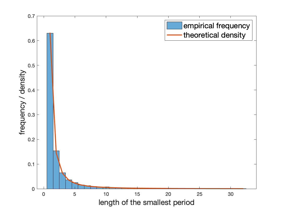
(a) $\sigma=1$, $n=100$

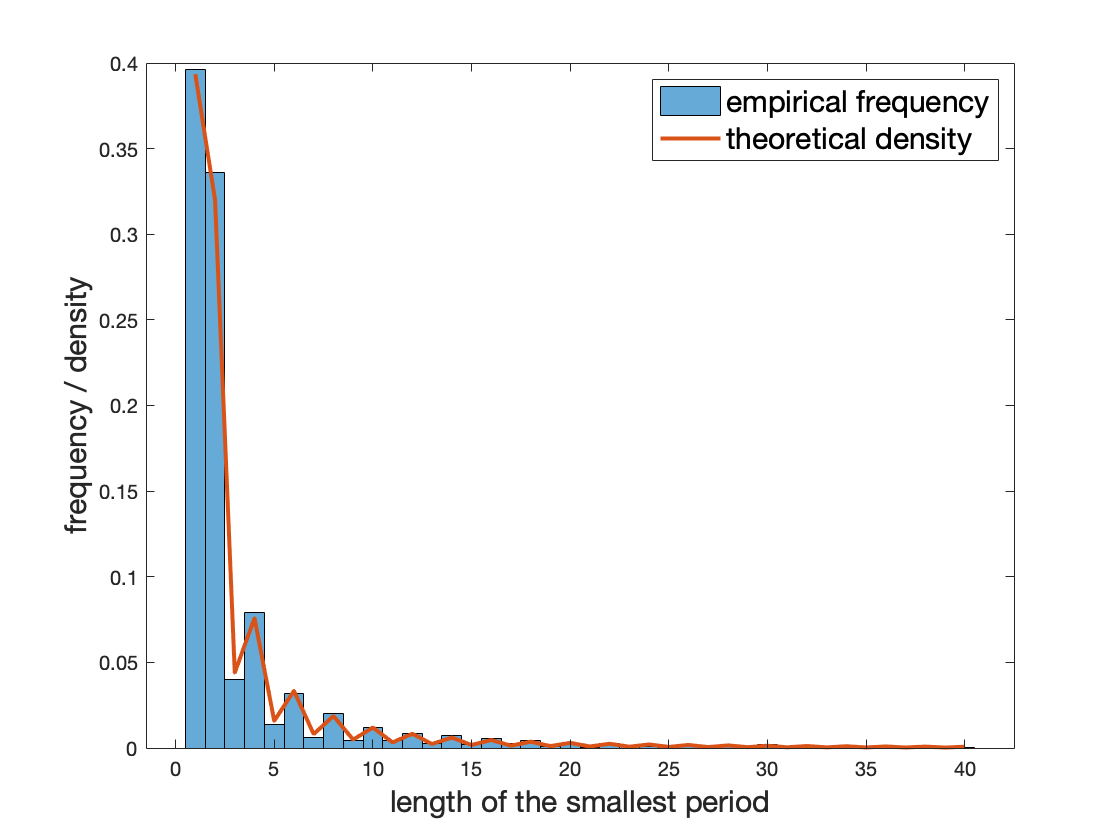
(b) $\sigma=2$, $n=100$

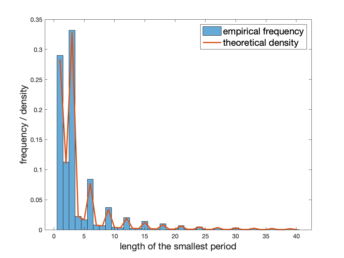
(c) $\sigma=3$, $n=60$

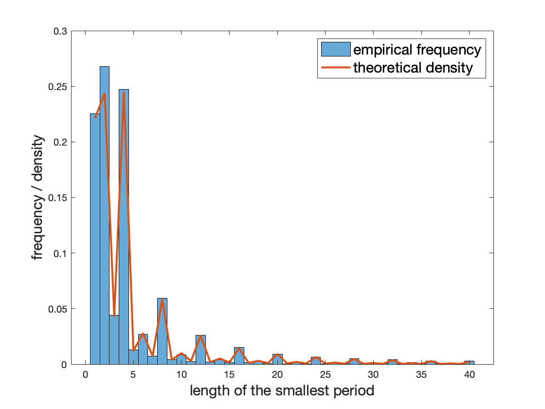
(d) $\sigma=4$, $n=20$

Figure 5: Lengths of the smallest temporal periods of PS with spatial periods $\sigma=1$ to $\sigma=4$ and various $n$. In each case, a histogram from a random sample from 10,000 rules is compared to the theoretical limiting distribution as $n\to\infty$, given by Corollary 3.

5 Discussion and open problems

In this paper, we initiate the study of periodic solutions for one-dimensional CA with random rules. Our main focus is the limiting probability of existence of a PS, when the rule is uniformly selected and the number of states approaches infinity, and we show (Corollary 3) that the smallest temporal period of PS with a given spatial period $\sigma$ is stochastically bounded.

By a similar argument, we can also obtain an analogous result in which we fix the temporal period instead of the spatial period. Define another random variable

$$Y_{\tau,n}^{\prime}=\min\{\sigma:\mathcal{P}_{\tau,\sigma,n}\neq\emptyset\},$$

which is the smallest spatial period of a PS given a temporal period $\tau$. For example, for the four rules in Figure 2, we may verify that, by Algorithm 2.8, $Y_{1,3}^{\prime}(\mathit{012200210})=1$ ($0\to 0$), $Y_{2,3}^{\prime}(\mathit{021102120})=2$ ($12\to 21\to 12$), $Y_{3,3}^{\prime}(\mathit{100112122})=3$ ($102\to 021\to 210\to 102$) and $Y_{4,3}^{\prime}(\mathit{101201021})=4$ ($0101\to 2012\to 1010\to 0122\to 0101$), with one cycle that generates the minimal PS given parenthetically for each case.

Corollary 4.

The random variable $Y_{\tau,n}^{\prime}$ converges to a nontrivial distribution as $n\to\infty$.

Perhaps the most natural generalization of Theorem 2 would relax the condition that $\mathcal{T}$ and $\Sigma$ are finite. The first case to consider surely is when either $\mathcal{T}=\mathbb{N}$ or $\Sigma=\mathbb{N}$. For example, it is clear that $\mathbb{P}(\mathcal{P}_{\mathbb{N},\mathbb{N},n}\neq\emptyset)=\mathbb{P}(\mathcal{P}_{\mathbb{N},\{1\},n}\neq\emptyset)=1$, as any constant initial configuration eventually generates a PS with spatial period 1.

Now, consider a general $\sigma\geq 2$. Let $\xi_{0}$ be a periodic configuration of spatial period $\sigma$. Under any CA rule $f$, $\xi_{1}$ maintains the spatial periodicity, hence $\xi_{t}$ eventually enters into a PS, whose spatial period is however a divisor of $\sigma$, not necessarily $\sigma$ itself. For this reason, we cannot reach an immediate conclusion about $\lim\mathbb{P}(\mathcal{P}_{\mathbb{N},\{\sigma\},n}\neq\emptyset)$, as $n\to\infty$. We also refer the readers to [7], in which the reduction of temporal periods is explored in more detail.

For a fixed temporal period $\tau$, the matter is even less clear as a rule may not have a PS with temporal period that divides $\tau$. For a trivial example with $\tau$ odd and $n=2$, consider the “toggle” rule that always changes the current state and thus $\xi_{t+1}=1-\xi_{t}$ and any initial state results in temporal period $2$. Thus we formulate the following intriguing open problem.

Question 5.1.

Let $\tau,\sigma\in\mathbb{N}$. What are the behaviors of $\mathbb{P}(\mathcal{P}_{\{\tau\},\mathbb{N},n}\neq\emptyset)$ and $\mathbb{P}(\mathcal{P}_{\mathbb{N},\{\sigma\},n}\neq\emptyset)$, as $n\to\infty$ ?

Another natural question addresses the case when $\sigma$ and $\tau$ increase with $n$.

Question 5.2.

For positive real numbers $a,b,c,d,\alpha,\beta,\gamma$ and $\delta$, what is the asymptotic behavior of $\mathbb{P}\left(\mathcal{P}_{I_{1},I_{2},n}\neq\emptyset\right)$, where $I_{1}=[an^{\alpha},bn^{\beta}]$ and $I_{2}=[cn^{\gamma},dn^{\delta}]$?

A wider topic for further research is to investigate how different the behavior of the shortest temporal period changes if we choose a random rule from a subset of the set of all rules. There are, of course, many possibilities for such a subset, and we selected two natural ones below. In each case, we denote the resulting random variable with the same letter $Y_{n,\sigma}$.

A rule is left permutative if the map $\psi_{b}:\mathbb{Z}_{n}\to\mathbb{Z}_{n}$ given by $\psi_{b}(a)=f(a,b)$ is a permutation for every $b\in\mathbb{Z}_{n}$. Permutative rules, such as the famous Rule 30 [18, 8], are good candidates for generation of long temporal periods.

Question 5.3.

Let $\mathcal{L}$ be the set of all $(n!)^{n}$ permutative rules. Choosing one of these rules uniformly at random from $\mathcal{L}$, what is the asymptotic behavior of $Y_{n,\sigma}$?

Our final question concerns the most widely studied special class of CA, the additive rules [13]. Such a rule is given by $f(a,b)=\alpha a+\beta b$, for some $\alpha,\beta\in\mathbb{Z}_{n}$.

Question 5.4.

Let $\mathcal{A}$ be the set of all $n^{2}$ additive rules. Again, what is the asymptotic behavior of $Y_{n,\sigma}$ if a rule from $\mathcal{A}$ is chosen uniformly at random?

References

- [1] Andrew D. Barbour, Lars Holst, and Svante Janson. Poisson approximation. Clarendon Press, 1992.
- [2] Mike Boyle and Bruce Kitchens. Periodic points for onto cellular automata. Indagationes Mathematicae, 10(4):483–493, 1999.
- [3] Mike Boyle and Bryant Lee. Jointly periodic points in cellular automata: computer explorations and conjectures. Experimental Mathematics, 16(3):293–302, 2007.
- [4] Raul Cordovil, Rui Dilão, and Ana Noronha da Costa. Periodic orbits for additive cellular automata. Discrete & Computational Geometry, 1(3):277–288, 1986.
- [5] Janko Gravner and David Griffeath. Robust periodic solutions and evolution from seeds in one-dimensional edge cellular automata. Theoretical Computer Science, 466:64, 2012.
- [6] Janko Gravner and Xiaochen Liu. Maximal temporal period of a periodic solution generated by a one-dimensional cellular automaton. In preparation, 2019.
- [7] Janko Gravner and Xiaochen Liu. One-dimensional cellular automata with random rules: longest temporal period of a periodic solution. In preparation, 2019.
- [8] Erica Jen. Global properties of cellular automata. Journal of Statistical Physics, 43(1–2):219–242, 1986.
- [9] Erica Jen. Cylindrical cellular automata. Communications in Mathematical Physics, 118(4):569–590, 1988.
- [10] Erica Jen. Linear cellular automata and recurring sequences in finite fields. Communications in Mathematical Physics, 119(1):13–28, 1988.
- [11] Jae-Gyeom Kim. On state transition diagrams of cellular automata. East Asian Math. J, 25(4):517–525, 2009.
- [12] Xiaochen Liu. Cellular automata with random rules. PhD thesis, University of California, Davis, in preparation, 2019.
- [13] Olivier Martin, Andrew M. Odlyzko, and Stephen Wolfram. Algebraic properties of cellular automata. Communications in mathematical physics, 93(2):219–258, 1984.
- [14] Michał Misiurewicz, John G. Stevens, and Diana M. Thomas. Iterations of linear maps over finite fields. Linear algebra and its applications, 413(1):218–234, 2006.
- [15] Nathan Ross. Fundamentals of stein’s method. Probability Surveys, 8:210–293, 2011.
- [16] John G. Stevens. On the construction of state diagrams for cellular automata with additive rules. Information Sciences, 115(1-4):43–59, 1999.
- [17] John G. Stevens, Ronald E. Rosensweig, and A. E. Cerkanowicz. Transient and cyclic behavior of cellular automata with null boundary conditions. Journal of statistical physics, 73(1-2):159–174, 1993.
- [18] Stephen Wolfram. Random sequence generation by cellular automata. Advances in Applied Mathematics, 7(2):132–169, 1986.
- [19] Stephen Wolfram. A new kind of science, volume 5. Wolfram media Champaign, IL, 2002.
- [20] Xu Xu, Yi Song, and Stephen P. Banks. On the dynamical behavior of cellular automata. International Journal of Bifurcation and Chaos, 19(04):1147–1156, 2009.