UCI–TR–2019–22

TUM–HEP 1223/19

A note on the predictions of models with modular flavor symmetries

Mu–Chun Chen^a, Saúl Ramos–Sánchez^b,c, Michael Ratz^a

^a Department of Physics and Astronomy, University of California, Irvine, CA 92697-4575 USA

^bInstituto de Física, Universidad Nacional Autónoma de México, POB 20-364, Cd.Mx. 01000, México
^cPhysik Department T75, Technische Universität München, James-Franck-Straße 1, 85748 Garching, Germany

Models with modular flavor symmetries have been thought to be highly predictive. We point out that these predictions are subject to corrections from non–holomorphic terms in the Lagrangean. Specifically, in the models discussed in the literature, the Kähler potential is not fixed by the symmetries, for instance. The most general Kähler potential consistent with the symmetries of the model contains additional terms with additional parameters, which reduce the predictive power of these constructions. We also comment on how one may conceivably retain the predictivity.

1 Introduction

Recently a rather exciting observation has been made [1, 2]: nine neutrino parameters can be predicted from only three input parameters. The crucial ingredients of the corresponding model are modular flavor symmetries. The point of this paper is to show that these models actually have additional parameters which have not been taken into account in the models in the recent literature. We also comment on possible ways to retain control over these parameters.

To understand the main point of our paper, recall that the predictions of these models come from the fact that the superpotential is fixed by the modular transformations. However, the superpotential only contains the physical parameters if the fields appearing there are “physical”, i.e. canonically normalized. As we shall see, the Kähler potential, which contains the information about the fields, is not at all fixed by the symmetries and transformation properties of the models. This is why the modular transformations alone do not allow one to make such remarkable predictions, as we shall discuss in more detail in what follows.

2 Modular flavor symmetries

Modular flavor symmetries have so far only been discussed in the supersymmetric context. There, they are modular transformations which act on a so–called modulus $\tau$ and “matter” superfields $\varphi^{(j)}$ according to [1]

$$\tau ~{}\mapsto~{}\frac{a\,\tau+b}{c\,\tau+d}~{}=:~{}\gamma\,\tau\;,$$ (1a)

$$\phi^{(j)} ~{}\mapsto~{}(c\,\tau+d)^{-k_{j}}\,\rho^{(j)}(\gamma)\,\phi^{(j)}\;,$$ (1b)

where $a$, $b$, $c$ and $d$ are the $\Gamma\equiv\mathrm{SL}(2,\mathbbm{Z})$ parameters satisfying, by definition, $a\,d-b\,c=1$ and $\rho^{(j)}$ is the representation matrix of some quotient group $\Gamma_{N}=\Gamma/\Gamma(N)$. $-k_{j}$ denotes the so–called modular weight. The collection of chiral superfields will be denoted $\Phi=(\tau,\phi^{(1)},\ldots,\phi^{(F)})$.

The modular group $\overline{\Gamma}=\Gamma/\mathbbm{Z}_{2}$ is generated by

$$S~{}=~{}\begin{pmatrix}0&1\\ -1&0\end{pmatrix}\quad\text{and}\quad T~{}=~{}\begin{pmatrix}1&1\\ 0&1\end{pmatrix}\;,$$ (2)

which correspond to the transformations

$$\tau~{}\xmapsto{~{}S~{}}~{}-\frac{1}{\tau}\quad\text{and}\quad\tau~{}\xmapsto{~{}T~{}}~{}\tau+1\;.$$ (3)

These generators satisfy

$$S^{2}~{}=~{}(S\,T)^{3}~{}=~{}\mathbbm{1}\;.$$ (4)

It is straightforward to verify that

$$\left(-\mathrm{i}\,\tau+\mathrm{i}\,\bar{\tau}\right)^{-k} ~{}\xmapsto{(\ref{eq:ModularTrafo})}~{}\left(\left(c\,\tau+d\right)\,\left(c\,\bar{\tau}+d\right)\right)^{k}\,\left(-\mathrm{i}\,\tau+\mathrm{i}\,\bar{\tau}\right)^{-k}\;.$$ (5)

Therefore, the combination

$$\left(-\mathrm{i}\,\tau+\mathrm{i}\,\bar{\tau}\right)^{-k_{j}}\,\left(\phi^{(j)*}\phi^{(j)}\right)_{\boldsymbol{1}}$$ (6)

is invariant under modular transformations. Here, the notation $\left(\cdots\right)_{\boldsymbol{1}}$ indicates a contraction to a $\Gamma_{N}$ $\boldsymbol{1}$–plet, i.e. to an invariant under $\Gamma_{N}$. However, as we shall see below, this is not the only invariant.

3 Additional parameters from non–holomorphic terms

The fact that there are additional terms in the Kähler potential has been already noted in [1]. The existence of additional terms already follows from the observation that the predicted parameters run. Running of couplings in supersymmetric theories can be understood as corrections to the Kähler potential. On the other hand, the superpotential is protected by holomorphicity, which is reflected by the non–renormalization theorems. As we shall see, the most general Kähler potential consistent with the symmetries has numerous additional parameters.

We will base our discussion on Model 1 of [1], which has the finite quotient symmetry $\Gamma_{3}\simeq A_{4}$. However, the analogous statements apply to the follow–up models in the literature such as [2, 3, 4, 5, 6, 7, 8, 9]. The Higgs and lepton sector of the model is specified in table 1.

$\begin{array}[]{|*{6}{c|}|c|}\hline\cr&(E_{1}^{c},E_{2}^{c},E_{3}^{c})&N&L&H_{d}&H_{u}&\varphi\\ \hline\cr\mathrm{SU}(2)_{\mathrm{L}}\times\mathrm{U}(1)_{Y}&\boldsymbol{1}_{1}&\boldsymbol{1}_{0}&\boldsymbol{2}_{-\nicefrac{{1}}{{2}}}&\boldsymbol{2}_{-\nicefrac{{1}}{{2}}}&\boldsymbol{2}_{\nicefrac{{1}}{{2}}}&\boldsymbol{1}_{0}\\ \hline\cr\Gamma_{3}&(\boldsymbol{1},\boldsymbol{1^{\prime}},\boldsymbol{1^{\prime\prime}})&\boldsymbol{3}&\boldsymbol{3}&\boldsymbol{1}&\boldsymbol{1}&\boldsymbol{3}\\ \hline\cr k&(k_{E_{1}},k_{E_{2}},k_{E_{3}})&k_{N}&k_{L}&k_{H_{d}}&k_{H_{u}}&k_{\varphi}\\ \hline\cr\end{array}$

Table 1: Model 1 of [1]. $E_{i}^{c}$, $L$, $H_{u}$ and $H_{d}$ are the superfields of the charged leptons, left–handed douplets, up–type Higgs and down–type Higgs, respectively.

As the author of [1] has pointed out, the charged fermion masses are obtained by adjusting three parameters. The nontrivial predictions of this model are on the neutrino parameters, which come form the Weinberg operator

$$\mathscr{W}_{\nu}~{}=~{}\frac{1}{\Lambda}\left[\left(H_{u}\cdot L\right)\,Y\,\left(H_{u}\cdot L\right)\right]_{\boldsymbol{1}}\;.$$ (7)

Here, $Y$ is a triplet of modular functions of weight 2, $Y=\left(Y_{1},Y_{2},Y_{3}\right)^{T}$. The Kähler potential of the charged leptons is taken to be

$$K_{L}~{}=~{}\left(-\mathrm{i}\,\tau+\mathrm{i}\,\bar{\tau}\right)^{-1}\,L^{\dagger}\,L\;.$$ (8)

Here the modular weights of the leptons are $-1$ (corresponding to $k_{L}=1$) and $H_{u}$ has zero weight ($k_{H_{u}}=0$). The neutrino mass matrix is then given by

$$m_{\nu}~{}=~{}\frac{v_{u}^{2}}{\Lambda}\begin{pmatrix}2Y_{1}(\tau)&-Y_{3}(\tau)&-Y_{2}(\tau)\\ -Y_{3}(\tau)&2Y_{2}(\tau)&-Y_{1}(\tau)\\ -Y_{2}(\tau)&-Y_{1}(\tau)&2Y_{3}(\tau)\end{pmatrix}\;.$$ (9)

The crucial point is that this matrix has only three free real parameters: $\Lambda$, $\operatorname{Re}\tau$ and $\operatorname{Im}\tau$. On the other hand, the charged lepton Yukawa coupling is diagonal in this model. Therefore, the mass matrix (9) fixes nine observables: the three neutrino mass eigenvalues, three mixing angles, the so–called Dirac $\mathcal{CP}$ phase and two Majorana phases. In [1, 2] values of $\tau$ that gives rise to realistic neutrino masses and mixing angles are specified. This is a spectacular result. Three real input parameters, $\Lambda$, $\operatorname{Re}\tau$ and $\operatorname{Im}\tau$, pin down three mass eigenvalues, three mixing angles and three phases. That is, this setting appears to make six nontrivial predictions, which agree amazingly well with observation (so far).

In more detail, the MNS matrix is the mismatch of the unitary transformations that diagonalize the neutrino mass matrix and the charged lepton Yukawa coupling matrix, respectively,

$$U_{\nu}^{T}\,m_{\nu}\,U_{\nu}~{}=~{}\operatorname{diag}(m_{1},m_{2},m_{3})\quad\text{and}\quad U^{\dagger}_{e_{\mathrm{L}}}\,Y_{e}\,Y_{e}^{\dagger}\,U_{e_{\mathrm{L}}}~{}=~{}\operatorname{diag}(y_{e}^{2},y_{\mu}^{2},y_{\tau}^{2})\;.$$ (10)

That is, $U_{\mathrm{MNS}}^{(0)}=U_{e_{\mathrm{L}}}\,U_{\nu}^{T}$, and since in the original Lagrangean $Y_{e}$ is diagonal, $U_{\mathrm{MNS}}^{(0)}=U_{\nu}^{T}$. The first term depends on nine physical parameters,

$$m_{\nu}~{}=~{}U_{\nu}^{*}\,\operatorname{diag}(m_{1},m_{2},m_{3})\,U_{\nu}^{\dagger}\;,\quad\text{where}~{}U_{\nu}=U_{\nu}(\theta_{12},\theta_{13},\theta_{23},\delta,\varphi_{1},\varphi_{2},\dots)$$ (11)

with $\theta_{ij}$ denoting the three mixing angles, $\delta$ the Dirac $\mathcal{CP}$ phase, $\varphi_{i}$ the two Majorana phases, and the omission “$\dots$” stands for three unphysical phases.

This parameter counting assumes that the Kähler potential is given by (8). However, the modular symmetries do not fix the form of the Kähler potential. Rather, the full Kähler potential includes additional terms beyond the one given in (8),

$$K ~{}=~{}\alpha_{0}\,\left(-\mathrm{i}\,\tau+\mathrm{i}\,\bar{\tau}\right)^{-1}\,\left(\overline{L}\,L\right)_{\boldsymbol{1}}+\sum_{k=1}^{7}\alpha_{k}\left(-\mathrm{i}\,\tau+\mathrm{i}\,\bar{\tau}\right)\,\left(Y\,L\,\overline{Y}\,\overline{L}\right)_{\boldsymbol{1},\,k}+\dots\;.$$ (12)

Here we have summed over all singlet contractions (specified by subscript $k$), and $\alpha_{0}$ can be absorbed in a redefinition of the fields. Some of the relevant contractions are given by $\left\{\left(\overline{Y}\,\overline{L}\right)_{\boldsymbol{3}^{(j)}}^{T}\left(Y\,L\right)_{\boldsymbol{3}^{(i)}}\right\}_{i,j\in\{1,2\}}$ and the invariant contractions of the one–dimensional contractions $\left(Y\,L\right)_{\boldsymbol{1},\boldsymbol{1}^{\prime},\boldsymbol{1}^{\prime\prime}}$ with appropriate conjugates. Specifically, the first three terms in the expansion (12) are

$$\Delta K~{}=~{} \alpha_{1}\,\left(\overline{Y}\,\overline{L}\right)_{\boldsymbol{3}^{(1)}}^{T}\left(Y\,L\right)_{\boldsymbol{3}^{(1)}}+\alpha_{2}\,\left(\overline{Y}\,\overline{L}\right)_{\boldsymbol{3}^{(2)}}^{T}\left(Y\,L\right)_{\boldsymbol{3}^{(2)}}$$

$${}+\alpha_{3}\,\left[\left(\overline{Y}\,\overline{L}\right)_{\boldsymbol{3}^{(1)}}^{T}\left(Y\,L\right)_{\boldsymbol{3}^{(2)}}+\left(\overline{Y}\,\overline{L}\right)_{\boldsymbol{3}^{(2)}}^{T}\left(Y\,L\right)_{\boldsymbol{3}^{(1)}}\right]+\ldots\;.$$ (13)

Note that all the terms are on the same footing, there is a priori no reason why, say, the $\alpha_{0}$ term should be referred to as the leading term and the others as “corrections”.

Once we add the other fields of the model, even more terms will have to be added. For instance, the above model [1, 2] also introduces a flavon $\varphi$ (cf. Table 1). Therefore, we can add further terms to the Kähler potential of the form

$$\Delta K ~{}=~{}\sum_{i}\beta_{i}\left(-\mathrm{i}\,\tau+\mathrm{i}\,\bar{\tau}\right)^{-k_{L}-k_{\varphi}}\,\left(\varphi\,L\,\overline{\varphi}\,\overline{L}\right)_{\boldsymbol{1},\,i}\;,$$ (14)

where we sum over all $A_{4}$–invariant contractions.

The impacts of these additional terms can be significant. Suppose one has derived predictions on the neutrino parameters based on the Kähler potential (8). The additional terms will modify the Kähler metric,

$$K^{i\bar{\jmath}}_{L}~{}=~{}\frac{\partial^{2}K}{\partial L_{i}\,\partial\overline{L}_{\bar{\jmath}}}\;.$$ (15)

This metric has to be diagonalized,

$$K_{L}~{}=~{}U_{L}^{\dagger}\,D^{2}\,U_{L}\;,$$ (16)

where $U_{L}$ is unitary and $D$ is diagonal and positive. Therefore, the canonically normalized fields are

$$\widehat{L}~{}=~{}D\,U_{L}\,L\quad\text{or equivalently}\quad L~{}=~{}U_{L}^{\dagger}\,D^{-1}\,\widehat{L}\;.$$ (17)

After adding the $\alpha_{i>0}$ contributions and transforming the fields back to canonical normalization, we need to diagonalize

$$\widehat{U}_{\nu}^{T}\,D^{-1}\,U_{L}^{*}\,m_{\nu}\,U_{L}^{\dagger}\,D^{-1}\,\widehat{U}_{\nu}~{} =~{}\operatorname{diag}(m_{1},m_{2},m_{3})\;,$$ (18a)

$$\widehat{U}_{e}^{\dagger}\,D^{-1}\,U_{L}^{*}\,Y_{e}\,Y_{e}^{\dagger}\,U_{L}^{T}\,D^{-1}\,\widehat{U}_{e}~{} =~{}\operatorname{diag}(y_{e}^{2},y_{\mu}^{2},y_{\tau}^{2})\;.$$ (18b)

This is to be compared with (10). We see that if $D$ is proportional to the unit matrix, there would be no effect, i.e.  the original mixing matrix $U_{\text{L}}$ would still do the job of diagonalizing $m_{\nu}$ and thus the predicted values for the neutrino mixing parameters based solely on $\alpha_{0}$ contribution remain valid. However, for the contributions given in (12), $D$ is generically not proportional to the unit matrix, and consequently the predicted values for the mixing angles get modified significantly. Our numerical analysis reveals that they are of the order

$$\Delta\theta_{ij}^{(k)}~{}=~{}\alpha_{k}\cdot(1\dots 10)^{\circ}\;,$$ (19)

and similarly for the $\mathcal{CP}$ phases. This is illustrated in Figure 1 for $k=3$.

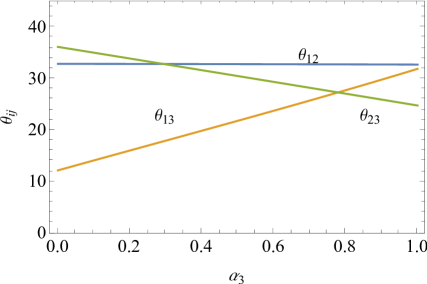
Figure 1: Dependence of the mixing angles on the additional parameter $\alpha_{3}$ (cf. Equation 13).

Analytic formulae that allow one to evaluate the impact of these corrections have been derived in [10, 11]. They confirm our result as given in (19). Importantly, these corrections are in general much larger than the corrections from RGE running and supersymmetry breaking which have been worked out in [2].

Altogether we see that in models with modular flavor symmetries the specification of $\tau$ and $\Lambda$ is not sufficient to determine the neutrino parameters. There exist many additional parameters, and, as a consequence, the number of free parameters is generically larger than the number of predictions.

4 Discussion

The findings of the previous section should not be surprising. The salient properties of the models with modular flavor symmetries rely on the holomorphicity of the superpotential. However, the Kähler potential does not have these properties. Moreover, these symmetries are nonlinearly realized.

How can one conceivably control the Kähler potential better? This will be possible if one derives the modular flavor symmetries from some more complete setting. As is well known, these symmetries come from tori. Thus one expects that there will be interpretations of these symmetries in models with extra dimensions.

Most prominently, modular symmetries appear in string theory. The existence of some non–Abelian symmetries has been already noted in [12], and more recently studied in more detail in [13, 14]. In particular, the $\mathbbm{Z}_{3}$ orbifold, which also has (in the absence of so–called discrete Wilson lines) a $\Delta(54)$ flavor symmetry [15], has a $\text{T}^{\prime}$ modular flavor symmetry [14]. Given these results, it is tempting to speculate that an $A_{4}$ modular flavor symmetry could originate from the $\mathbb{T}^{2}/\mathbbm{Z}_{2}$ orbifold, where the four twisted string states form a $(\boldsymbol{3}+\boldsymbol{1})$ reducible representation.

Note that in string theory, the notation is usually somewhat different (cf. e.g. [16]). Instead of denoting the modulus $\tau$ and demanding that its imaginary part transforms as a real scalar and its real part as a pseudoscalar, many string theorists prefer to consider $T$ instead of $\tau=\mathrm{i}\,T$. Then the real part transforms as scalar and has often the interpretation of volume. The imaginary part is sometimes referred to as $T$–axion. The transformation of $T$ and the matter fields under $\gamma\in\Gamma_{N}$ then reads

$$T ~{}\mapsto~{}\frac{a\,T-\mathrm{i}\,b}{\mathrm{i}\,c\,T+d}\;,$$ (20a)

$$\varphi^{(j)} ~{}\mapsto~{}\left(\mathrm{i}\,c\,T+d\right)^{n_{j}}\,\rho^{(j)}(\gamma)\,\varphi^{(j)}\;,$$ (20b)

where the $n_{j}=-k_{j}$ are the modular weights.

In contrast to the bottom–up models, in many string theory compactifications the modular weights are not free parameters but can be computed from other data of the models. They are used to derive approximate expressions for the Kähler potential. For example, by considering string scattering amplitudes in heterotic orbifold compactifications (although this result is more general; see e.g. [17]) and the so–called large volume limit $\operatorname{Re}T\gg 1$, it has been found that the leading contribution to the Kähler potential for the matter fields is given by [18]

$$K~{}\supset~{}\sum_{\ell}F_{i\ell}^{*}(\overline{T})F_{\ell j}(T)\left(T+\overline{T}\right)^{n_{j}}\,\overline{\varphi}^{(i)}\varphi^{(j)}\,,$$ (21)

where the modular weights $n_{j}$ are derived from the oscillator quantum numbers and the twist of the fields $\varphi^{(j)}$, and turn out to be (mostly) nonpositive. $F_{\ell j}$ are arbitrary holomorphic functions, building a non–degenerate matrix that fix the basis of the field space. Although these functions are typically chosen as $F_{\ell j}=\delta_{\ell j}$ for all $j$ and $\ell$, one may in principle also consider modular forms of nontrivial modular weight $n_{F_{\ell j}}$. Modular invariance of the Kähler potential would then imply that $n_{j}$ must be replaced by $n_{j}+n_{F_{\ell j}}$ in Equation 21. If we suppose that $F_{\ell j}=\delta_{\ell j}Y(T)$ for $\varphi^{(j)}=L$, the terms of the Kähler potential (12) with $k\neq 0$ are recovered with no additional suppression. Note however that the functions $F_{\ell j}$ can be absorbed in field redefinitions at the expense of altering the superpotential couplings.

It is known that the Kähler potential (21) receives additional contributions (see e.g. [19]). E.g. for string compactifications where matter arises from bulk fields, the Kähler potential can be expressed as $K=-\ln(T+\overline{T}-|\varphi^{(j)}|^{2})$, which yields (6) only in the large volume limit. However, the best–fit point for phenomenology in the model discussed ($\operatorname{Re}T\approx 1$) violates this limit. It should also be noted that in string compactifications the superpotential usually transforms nontrivially, and has modular weight $-1$.

Furthermore, as is well known, string theory is in principle very predictive. However, in concrete examples it is nontrivial to make precise predictions. This is because string models leave us typically with several moduli, whose potential is hard to explicitly compute and to minimize. Therefore it might be worthwhile to derive modular flavor symmetries from less complex settings, such as magnetized tori, where the background fluxes lead to chiral fermions [20]. Such models seem to give rise to modular flavor symmetries of the type discussed in this note [5]. These models are dual to $D$–brane models [21], and the couplings there can be mapped to couplings on orbifolds [22].

All these arguments suggest that more efforts need to go into deriving the modular flavor symmetries from string theory, or other higher–dimensional models. It is only then one might control the Kähler potential well enough to make controlled predictions.

As a side remark, let us also comment on the terminology. In some of the recent literature, the transformation

$$\mathscr{W}(\Phi) ~{}\mapsto~{}\mathscr{W}(\Phi)\;,$$ (22a)

$$K(\Phi,\overline{\Phi}) ~{}\mapsto~{}K(\Phi,\overline{\Phi})+f(\Phi)+\bar{f}(\overline{\Phi})\;,$$ (22b)

where $f$ is a holomorphic function, is referred to as “Kähler transformation”. Since the Lagrangean of a supersymmetric theory is given by

$$\mathscr{L}~{}=~{}\int\!\mathrm{d}^{4}\theta\,K(\Phi,\overline{\Phi})+\left[\int\!\mathrm{d}^{2}\theta\,\mathscr{W}(\Phi)+\text{h.c.}\right]\;,$$ (23)

we note that it is invariant under (22) just because

$$\int\!\mathrm{d}^{4}\theta\,f(\Phi)~{}=~{}\int\!\mathrm{d}^{4}\theta\,\bar{f}(\overline{\Phi})~{}=~{}0\;.$$ (24)

So (22) is nothing but the statement that one can shift the Kähler potential of a global supersymmetric theory by the real part of a holomorphic function without changing a Lagrangean. This is not a Kähler true transformation. Kähler transformations are formally written as [23]

$$\mathscr{W}(\Phi) ~{}\mapsto~{}\mathrm{e}^{-f(\Phi)}\,\mathscr{W}(\Phi)\;,$$ (25a)

$$K(\Phi,\overline{\Phi}) ~{}\mapsto~{}K(\Phi,\overline{\Phi})+f(\Phi)+\bar{f}(\overline{\Phi})\;.$$ (25b)

They have the virtue of leaving the scalar potential

$$\mathscr{V}_{\mathrm{SUGRA}}~{}=~{}\mathrm{e}^{K}\,\left[K^{i\bar{\jmath}}\left(D_{i}\mathscr{W}\right)\,\left(\overline{D}_{\bar{\jmath}}\overline{\mathscr{W}}\right)-3|\mathscr{W}|^{2}\right]$$ (26)

invariant. The Kähler transformation (25) does reduce to (22) for dimensionful fields $\Phi$ at zeroth order in $\Phi/\Lambda$ because of the suppression scale $\Lambda$ in the exponent of $e^{-f}$. However, for dimensionless fields, such as $\Phi=T$ (or $\tau$) (cf. [1, footnote 3]), no such suppression appears and thus only (25) is a proper Kähler transformation in this context. As mentioned above, it does not make sense to expand in $T/\Lambda$, i.e. the point in field space at which $|T|$ is small is not a point one may expand around. This observation becomes relevant in constructions emerging from string theory, where the Kähler transformations (25), and not (22), are symmetries of the theory.

5 Summary

Motivated by the striking observation that modular flavor symmetries allow one, at some level, to successfully make several nontrivial predictions [1, 2], we have studied these models in some more detail. We find that there are additional parameters which have not been taken into account in the literature so far. The existence of these parameters renders these models less predictive than previously thought.

Let us emphasize, though, that despite the existence of additional parameters, the modular flavor symmetries continue to be highly interesting approach to the flavor problem. It will be instrumental to derive them from a more complete setting, in which one may hope to control the Kähler potential to a greater degree.

Acknowledgments

It is a pleasure to thank Patrick Vaudrevange for useful discussions. The work of M.-C. C. was supported, in part, by the National Science Foundation, under Grant No. PHY-1915005. The work of S.R.-S. was partly supported by DGAPA-PAPIIT grant IN100217, CONACyT grants F-252167 and 278017, PIIF grant and the TUM August–Wilhelm Scheer Program. The work of M.R. is supported by NSF Grant No. PHY-1719438.

References

- [1] F. Feruglio, Are neutrino masses modular forms?, From My Vast Repertoire …: Guido Altarelli’s Legacy (A. Levy, S. Forte, and G. Ridolfi, eds.), 2019, pp. 227–266.
- [2] J. C. Criado and F. Feruglio, SciPost Phys. 5 (2018), no. 5, 042, arXiv:1807.01125 [hep-ph].
- [3] T. Kobayashi, N. Omoto, Y. Shimizu, K. Takagi, M. Tanimoto, and T. H. Tatsuishi, JHEP 11 (2018), 196, arXiv:1808.03012 [hep-ph].
- [4] P. P. Novichkov, J. T. Penedo, S. T. Petcov, and A. V. Titov, JHEP 04 (2019), 005, arXiv:1811.04933 [hep-ph].
- [5] T. Kobayashi and S. Tamba, Phys. Rev. D99 (2019), no. 4, 046001, arXiv:1811.11384 [hep-th].
- [6] F. J. de Anda, S. F. King, and E. Perdomo, arXiv:1812.05620 [hep-ph].
- [7] T. Kobayashi, Y. Shimizu, K. Takagi, M. Tanimoto, T. H. Tatsuishi, and H. Uchida, Phys. Lett. B794 (2019), 114, arXiv:1812.11072 [hep-ph].
- [8] G.-J. Ding, S. F. King, and X.-G. Liu, arXiv:1903.12588 [hep-ph].
- [9] T. Kobayashi, Y. Shimizu, K. Takagi, M. Tanimoto, and T. H. Tatsuishi, arXiv:1907.09141 [hep-ph].
- [10] M.-C. Chen, M. Fallbacher, M. Ratz, and C. Staudt, Phys. Lett. B718 (2012), 516, arXiv:1208.2947 [hep-ph].
- [11] M.-C. Chen, M. Fallbacher, Y. Omura, M. Ratz, and C. Staudt, Nucl. Phys. B873 (2013), 343, arXiv:1302.5576 [hep-ph].
- [12] S. Ferrara, D. Lüst, and S. Theisen, Phys. Lett. B233 (1989), 147.
- [13] A. Baur, H. P. Nilles, A. Trautner, and P. K. S. Vaudrevange, Phys. Lett. B795 (2019), 7, arXiv:1901.03251 [hep-th].
- [14] A. Baur, H. P. Nilles, A. Trautner, and P. K. S. Vaudrevange, arXiv:1908.00805 [hep-th].
- [15] T. Kobayashi, H. P. Nilles, F. Plöger, S. Raby, and M. Ratz, Nucl. Phys. B768 (2007), 135, hep-ph/0611020.
- [16] L. E. Ibáñez and D. Lüst, Nucl. Phys. B382 (1992), 305, hep-th/9202046.
- [17] J. P. Conlon, D. Cremades, and F. Quevedo, JHEP 01 (2007), 022, arXiv:hep-th/0609180 [hep-th].
- [18] V. Kaplunovsky and J. Louis, Nucl. Phys. B444 (1995), 191, arXiv:hep-th/9502077 [hep-th].
- [19] I. Antoniadis, E. Gava, K. S. Narain, and T. R. Taylor, Nucl. Phys. B432 (1994), 187, hep-th/9405024.
- [20] D. Cremades, L. E. Ibáñez, and F. Marchesano, JHEP 05 (2004), 079, hep-th/0404229.
- [21] D. Cremades, L. E. Ibáñez, and F. Marchesano, JHEP 07 (2003), 038, hep-th/0302105.
- [22] S. A. Abel and A. W. Owen, Nucl. Phys. B682 (2004), 183, hep-th/0310257.
- [23] J. Wess and J. Bagger, Supersymmetry and supergravity, Princeton University Press, Princeton, NJ, USA, 1992.